Deep learning for quality control of receiver functions

Receiver function has been routinely used for studying the discontinuity structure in the crust and upper mantle. The manual quality control of receiver functions, which plays a key role in high-quality data selection and accurate structural imaging, has been challenged by today’s booming data volumes. Traditional automatic quality control methods usually require tuning hyperparameters and fail to generalize to low signal-to-noise ratio data. Deep learning has been increasingly used to deal with extensive seismic data. However, it generally requires a manually labeled dataset, and its performance is highly related to the network design. In this study, we develop and compare four different deep learning network designs with manual and traditional quality control methods using 53293 receiver functions from three broadband seismic stations. Our results show that a combination of convolutional and long-short memory layers achieves the best performance of ∼91% accuracy. We also propose a fully automatic training schema that requires zero manually labeled receiver function yet achieves similar performance to that using carefully labeled ones. Compared with the traditional automatic method, our model retrieves ∼5 times more reliable receiver functions from relatively small earthquakes with magnitudes between 5.0 and 5.5. The average waveforms and H-κ stacking results of these receiver functions are comparable to those obtained by manual quality control from earthquakes with magnitudes larger than 5.5, which further demonstrates the validity of our method and indicates its potential for making use of smaller earthquakes in the receiver function analysis.

Introduction

Receiver function analysis can provide valuable constraints on the discontinuity structure in the crust and upper mantle, e.g., the Moho and the upper and lower boundaries of the mantle transition zone (Chen et al., 2010; Tauzin et al., 2010; Wei et al., 2016; Munch et al., 2020). Due to extensive noise in field seismograms, quality control is essential for obtaining high-quality receiver functions in practice. Although manually performing quality control can achieve high accuracy, it is time-consuming and subjective. Researchers have proposed several automatic quality control methods (Yang et al., 2016; Hassan et al., 2020). However, they generally require setting hyperparameters empirically. For example, Schulte-Pelkum et al. (2005) apply a minimum variance reduction as the final receiver function criterion, in which the conservative criterion risks rejecting a certain number of “good” receiver functions. Shen et al. (2012) apply harmonic stripping to quality control and analyze the receiver functions with a wide azimuthal distribution and azimuthal dependence of phase arrivals. Gao and Liu (2014) use the signal-to-noise ratio (SNR) cutoff to reject low SNR receiver functions, which do not consider the time and amplitude variations of phases. Similarly, Hassan et al. (2020) cluster the receiver functions by the Euclidean distance, which demands a certain amount of receiver functions per back-azimuth bin. Therefore, there is still considerable demand for improving quality control methods to characterize “good” receiver functions more efficiently in practice.

Different from the methods above that use only manually designed features for quality control, deep-learning-based methods can automatically extract abundant features from labeled receiver functions. Deep learning has made significant progress not only in the field of artificial intelligence over the last decade (LeCun et al., 2015), such as natural language processing and computer vision, but also in a variety of seismic applications (e.g., Kong et al., 2018; Zhou et al., 2021). In brief, deep learning aims to automatically build a mapping function from input to output with a given dataset. The parameters in the mapping function are initialized randomly and updated during training according to the gradients of the loss function. A validation dataset is generally used to avoid overfitting and determine when to stop training. In recent studies, deep-learning-based methods, such as convolution neural network (CNN), have been attempted to process the task of the quality control of receiver functions (Gan et al., 2021; Li et al., 2021). However, they still require time-consuming manual labeling of receiver functions as the training dataset and lack the comparison of the impact of model design on their performance.

In this study, we develop a fully automatic receiver function quality control method that achieves human-level performance via the following points: 1) we validate the effectiveness of our method and study the impact of the network design by developing and comparing four different deep neural network designs to both manual and traditional approaches; 2) we show its potential for smaller earthquakes by applying it to earthquakes with magnitudes between 5.0 and 5.5 and compare average waveforms and H-κ results to that using earthquakes with magnitudes above 5.5; 3) we investigate the generalizability between different stations by evaluating the models trained with different datasets; 4) we propose a workaround solution that requires zero manual labels. Because deep learning is naturally robust to noise (Rolnick et al., 2017), we evaluate the models trained with labels by the traditional method and show that deep learning can learn from these noisy labels and promote the results by the traditional method to the human level.

Methods

To investigate the effect of the manual design of the deep learning model on receiver function quality control, we compare the following four most widely-used layers in deep learning: 1) Fully connected layers that every neuron in the input layer to every neuron in the output layer are connected. They are conceptually and technically simple and thus suitable for baseline reference; 2) Convolutional layers that every output neuron is only connected to a local area of input neurons; They can significantly reduce the number of parameters than fully connected layers, and are widely used in image and time-series processing for feature extraction. The residual block contains two convolutional layers and learns residual functions with reference to the layer inputs (He et al., 2016); 3) Bidirectional long-short-memory layers that consist of two LSTM layers, each of which takes the input in a forward and backward direction, respectively (Hochreiter and Schmidhuber, 1997). They can capture dependencies between timestamps, and are potentially suitable for the receiver function quality control; 4) Transformer layers that consist of a self-attention layer and a position-wise feed-forward layer (Vaswani et al., 2017). They have attained state-of-the-art performance not only in neural language processing (Devlin et al., 2019) and computer vision (Dosovitskiy et al., 2020) but also in earthquake detection and phase picking (Mousavi et al., 2020). However, they generally require large amounts of data to train due to the lack of locality inductive bias (D’Ascoli et al., 2021).

We build four deep-learning models (Figure 1) according to the abovementioned four layers using the TensorFlow 2 framework (Abadi et al., 2016). The first model, namely the FC model, sorely consists of four fully-connected layers (Figure 1A). The second model, namely the CNN model, consists of three residual convolutional blocks (He et al., 2016) for feature extraction, followed by three fully-connected layers serving as the prediction head (Figure 1B). The third model, the CNN-BiLSTM model, adds a BiLSTM layer based on the second model (Figure 1C). The last model, the CNN-BiLSTM-Trans model, adds a transformer layer based on the third model (Figure 1D). All four models take a receiver function (windowed from 10s before to 50s after the P wave arrival) as the input, which is a tensor of a shape [600, 1]. And they all output a tensor of a shape [2], which is the one-hot encoding format of the classification results of “good” and “bad”. We apply a dropout rate of 0.5 for the FC model and 0.1 for the other three models in all layers except the final and the penultimate layers, and an early-stopping callback of 50-epoch-patience to ease the overfitting issue. The loss function used in all four models is cross-entropy, which is widely used in classification problems. In addition, to address the data imbalance issue, a balanced sampling strategy is used to keep the same number of “good” and “bad” instances in one batch. Details on training and validation are presented in the Results and Discussion section.

FIGURE 1

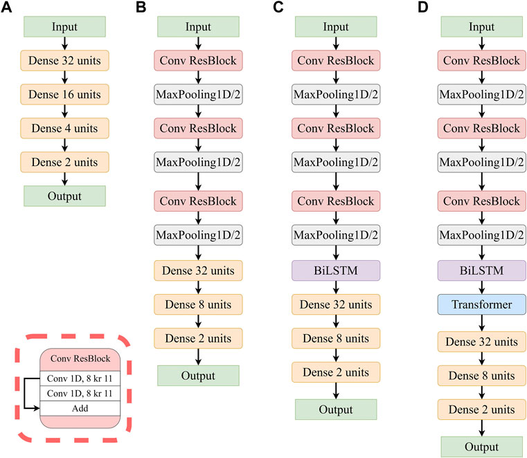
FIGURE 1. Diagrams of the four deep learning models. (A) FC model. (B) CNN model. (C) CNN-BiLSTM model. (D) CNN-BiLSTM-Trans model.

Data

We build the dataset using the earthquake catalog of Incorporated Research Institutions for Seismology (IRIS). We select earthquakes with magnitudes greater than 5.0 and download corresponding waveforms recorded by three stations (station AK. SAW, IC. QIZ, and CB. CAD located at 148.33° W/61.81° N, 109.84° E/19.03° N, and 97.5° E/31° N, respectively) with the criteria that epicentral distances are between 30° and 90° (Figure 2, Supplementary Figure S1). These stations have been in operation since around the year 2000. Three stations with different geological background and thus having different crustal structures are chosen to test the general applicability of the new method. According to the magnitude of the earthquakes, we divide the data from each station into two groups: those with magnitudes greater than 5.5 are used to compare different model designs, and those with magnitudes between 5.0 and 5.5 are used to evaluate our model’s performance on smaller earthquakes.

FIGURE 2

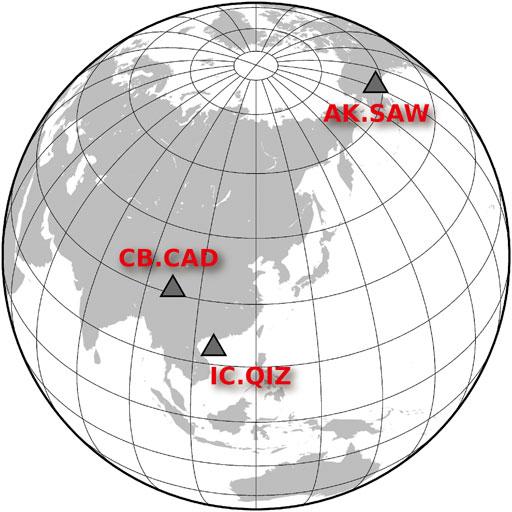
FIGURE 2. Location of station AK. SAW, station IC. QIZ and station CB. CAD.

Receiver functions are extracted in the following steps: 1) For each earthquake, three-component waveforms are windowed from 50 s before to 150 s after the P wave arrival and then rotated from a vertical-north-east coordinate system to a vertical-radial-transverse coordinate system; 2) Three-component waveforms are filtered using a Butterworth bandpass filter with a frequency band of 0.02–1 Hz; 3) Receiver functions are calculated by an iterative time-domain deconvolution method (Ligorría and Ammon, 1999). The width of the Gaussian filter window used in this study is 1.0; 4) Receiver functions containing null values or having an unexpected number of samples are removed. Finally, 12487 receiver functions (with magnitudes larger than 5.5) are selected as the training and validation sets to compare four model designs, and the other 40806 receiver functions (with magnitudes between 5.0 and 5.5) serve as a test set to evaluate the trained model’s performance on smaller earthquakes.

In the comparison experiment of model designs, we first manually label the quality of 12487 receiver functions (labels are “good” and “bad”) according to the principle that ones with similar back-azimuth have similar waveforms. The high SNR receiver functions labeled “good” have a clear direct P-wave signal and the Ps conversion from Moho. The receiver functions in the training set have good coverage of back-azimuth in order to include as many features as possible. The AK.SAW, IC.QIZ, CB.CAD datasets consist of 941, 771, 946 “good” receiver functions, and 4,515, 4,548, 748 “bad” receiver functions, respectively. We randomly split these receiver functions into training and validation sets with weights of 0.8 and 0.2, respectively. The back-azimuth of the test set exhibits the same wide distribution as the training and validation sets (Supplementary Figure S1). The performance on the test set is evaluated by comparing the phase time and amplitude with manually quality-controlled “good” receiver functions with magnitudes above 5.5.

Results and discussion

We first present the training and validation of four models on data from each station. As shown in Figure 3, all models tend to overfit (the training loss decreases while the validation loss increases) on the training set, which means early stopping is necessary for this task to ease the overfitting issue. As a result of evaluating the FC models with two, three, and four hidden layers, we find that all the three FC models end up overfitting, and we keep the three-layer one that achieves the best performance (Supplementary Figure S2 and Supplementary Table S1). The FC model obtains the lowest performance among four models on three station datasets (Table 1). Adding and removing layers from the current FC model does not further improve its performance (Supplementary Figure S2). The addition of the BiLSTM layer further improves the CNN model and achieves the best performance on the three validation datasets. The transformer layer does not further promote the model, suggesting it may not suit this task as it requires extensive training data.

FIGURE 3

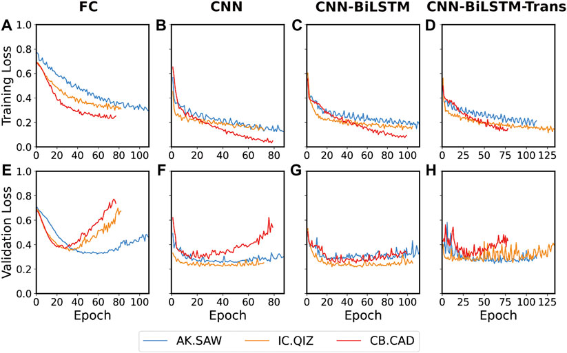
FIGURE 3. Training and validation loss of the four models on training sets of each station. (A,E) FC Model. (B,F) CNN model. (C,G) CNN-BiLSTM Model. (D,H) CNN-BiLSTM-Trans Model.

TABLE 1

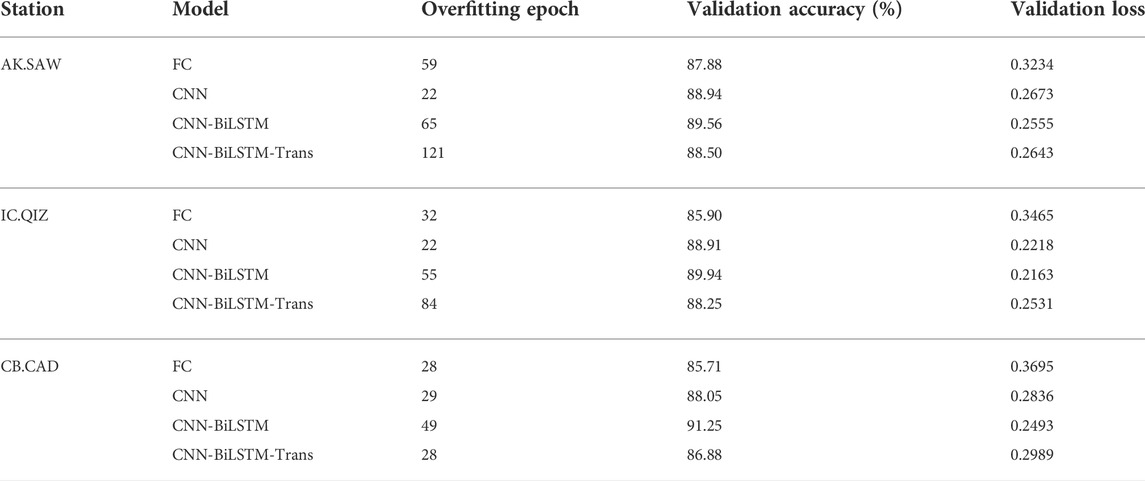
TABLE 1. The performance of the four model designs on the training and validation sets.

We choose each model with the minimum validation loss as the best model of its design. Then we visualize their stacked waveforms in each back-azimuth bin (Supplementary Figures S3–S5) and compute their classification confusion matrixes on the validation sets (Table 2). The confusion matrix consists of four values: 1) True positive (TP) that a “good” receiver function is classified as “good”; 2) True Negative (TN) that a “bad” is classified as “bad”; 3) False Positive (FP) that a “bad” is classified as “good”; 4) False Negative (FN) that a “good” is classified as “bad”. The confusion matrix can better represent the performance of the method in classification problems, especially for imbalanced datasets. The results show that the CNN-BiLSTM model exhibits the highest TP and TN rate and the lowest FP and FN rate in all the three station datasets, which indict the CNN-BiLSTM model has the best performance for quality control in practice. Overall, both the training and validation loss curve and the confusion matrix show that the CNN-BiLSTM model is the best among the four model designs. We also choose the traditional quality control method in HiPerSeis as a benchmark (Hassan et al., 2020), which is based on amplitude criteria and clustering receiver functions by similarity. The quality control method in HiPerSeis requires only two hyperparameters, which is comparable to the deep learning method that requires zero hyperparameters in terms of convenience. According to the experiment of tuning the distance threshold (Supplementary Table S2), the distance threshold and min samples used in DBSCAN clustering are 0.05 and 5, respectively. We apply this traditional method to the three station datasets with magnitudes above 5.5 and compute their classification confusion matrixes (Table 2). The results show that the FP rate is low, which means very few “bad” receiver functions may be mislabeled as “good” in practice. However, the TP rates are much lower compared to that of the CNN-BiLSTM model trained by manually quality controlled datasets, which means many “good” receiver functions may be wrongly discarded in practice.

TABLE 2

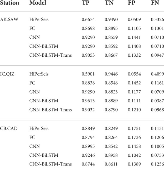
TABLE 2. Normalized confusion matrixes of the four deep learning models and traditional method (HiPerSeis) on three station datasets.

We further apply the trained CNN-BiLSTM model to the receiver function data from smaller earthquakes with magnitudes between 5.0 and 5.5 and compare its results to those obtained from the same earthquakes via HiPerSeis and those obtained from large earthquakes via manual quality control (Supplementary Figures S6–S8). The earthquakes less than 5.5 magnitude are generally discarded in receiver function analysis due to their low SNR, on which both manual and traditional quality controls tend to fail. However, these smaller magnitude earthquake data could increase the back-azimuth distribution, which is the premise for mapping dipping and anisotropic structures beneath a single station. In the AK. SAW dataset, 691 and 95 receiver functions are labeled as “good” by deep learning and traditional methods, respectively. And their patterns are consistent with those of manual quality control (Figures 4A–C, Supplementary Figures S6A–C). In the IC. QIZ dataset, 686 and 74 receiver functions are labeled as “good” by deep learning and traditional methods, respectively (Figures 4D–F, Supplementary Figures S7A–C). In the CB. CAD dataset, 458 and 265 receiver functions are labeled as “good” by deep learning and traditional methods, respectively (Figures 4G–I, Supplementary Figures S8A–C). Compared with the traditional method in HiPerSeis, our new method retrieves several times more reliable receiver functions, which possess a wider back-azimuth distribution (Figure 4, Supplementary Figures S6–S8). These “good” receiver functions have similar phase time and amplitude features to those from manual quality control (Figure 5). The average waveforms, including the time and amplitudes of phases such as direct P and conversion and multiple reflections from Moho, are almost identical for all the three quality controlled datasets (Figure 5). The result shows that the CNN-BiLSTM model can retrieve more reliable receiver functions from smaller earthquakes, which can increase the back-azimuth distribution.

FIGURE 4

FIGURE 4. Receiver functions stacked in each back-azimuth bin. (A–C) Three “good” AK. SAW datasets (manually quality controlled dataset with magnitudes larger than 5.5, automatically quality controlled dataset by the CNN-BiLSTM model with magnitudes between 5.0 and 5.5 and automatically quality controlled dataset by the traditional method in HiPerSeis with magnitudes between 5.0 and 5.5). The summational traces in the top panels. (D–F) are the same as (A–C) but for three “good” IC. QIZ datasets. (G–I) are the same as (A–C) but for three “good” CB. CAD datasets.

FIGURE 5

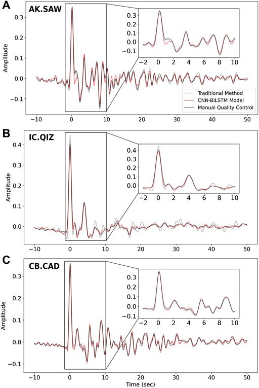
FIGURE 5. The average waveforms of the three datasets (manually quality controlled dataset with magnitudes larger than 5.5, automatically quality controlled dataset by the CNN-BiLSTM model with magnitudes between 5.0 and 5.5 and automatically quality controlled dataset by the traditional method in HiPerSeis with magnitudes between 5.0 and 5.5) recorded by (A) AK. SAW station, (B) IC. QIZ station, and (C) CB. CAD station.

We further validate the classification quality of the CNN-BiLSTM model with H-κ stacking, which is a receiver function method for estimating the crustal thickness and Vp/Vs. ratio beneath a seismic station (Zhu and Kanamori, 2000). This method stacks the amplitudes of receiver functions at predicted arrival times for the Ps phase and multiple phases. Here we give the weights of 0.5, 0.35, and 0.15 to the Ps, PpPs, and PpSs + PsPs phases when summing the amplitudes based on their magnitude of energy. The H-κ stacking is then applied to both the manually quality controlled datasets of bigger earthquakes (magnitude above 5.5) and the CNN-BiLSTM model quality controlled datasets of smaller earthquakes (magnitude between 5.0 and 5.5) (Figure 6 and Supplementary Figure S9). The obtained crustal thickness and Vp/Vs. ratio using receiver functions provided by the CNN-BiLSTM model are nearly identical as those estimated by the manually quality controlled dataset in three station datasets. The H-κ stacking results are consistent with the recent CCP imaging result and H-κ stacking results in the previous studies (Chen et al., 2010; Miller et al., 2018). This suggests that the CNN-BiLSTM model is highly reliable for receiver function quality control.

FIGURE 6

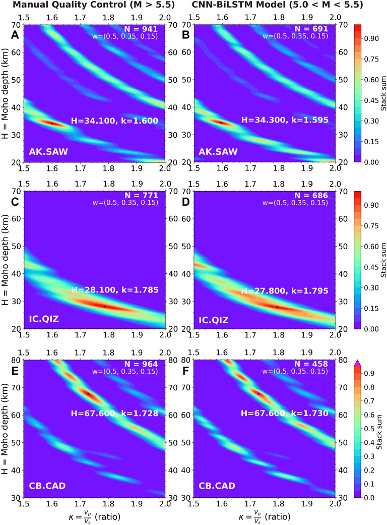
FIGURE 6. Thickness (H) versus Vp/Vs ratio (κ) diagrams from the H-κ stacking method for representative datasets. (A) Manually quality controlled station AK. SAW dataset with earthquake magnitudes larger than 5.5. (B) Automatically quality controlled station AK. SAW dataset by the CNN-BiLSTM model with earthquake magnitudes between 5.0 and 5.5. (C,D) are the same as (A,B) but for station IC. QIZ datasets. (E,F) are the same as (A,B) but for station CB. CAD datasets.

Although the previous experiments show that the deep learning method achieves results close to those by manual quality control, one significant limitation of the proposed deep learning method is that it requires a pre-existing manually quality controlled dataset for training, which is generally not available in the task of receiver function quality control. Here we propose a workaround solution: training the model with labels obtained by the traditional automatic method. Because deep learning is inherently robust to noise in training (Rolnick et al., 2017), it can still extract correct features even with the training dataset labeled by the traditional method (Table 3 and Supplementary Figures S10). The results show that the model trained with noisy datasets achieves comparable (slightly lower) performance to that trained with manually labeled datasets. That aside, this training schema allows our approach to be fully automated without requiring a pre-existing manual dataset.

TABLE 3

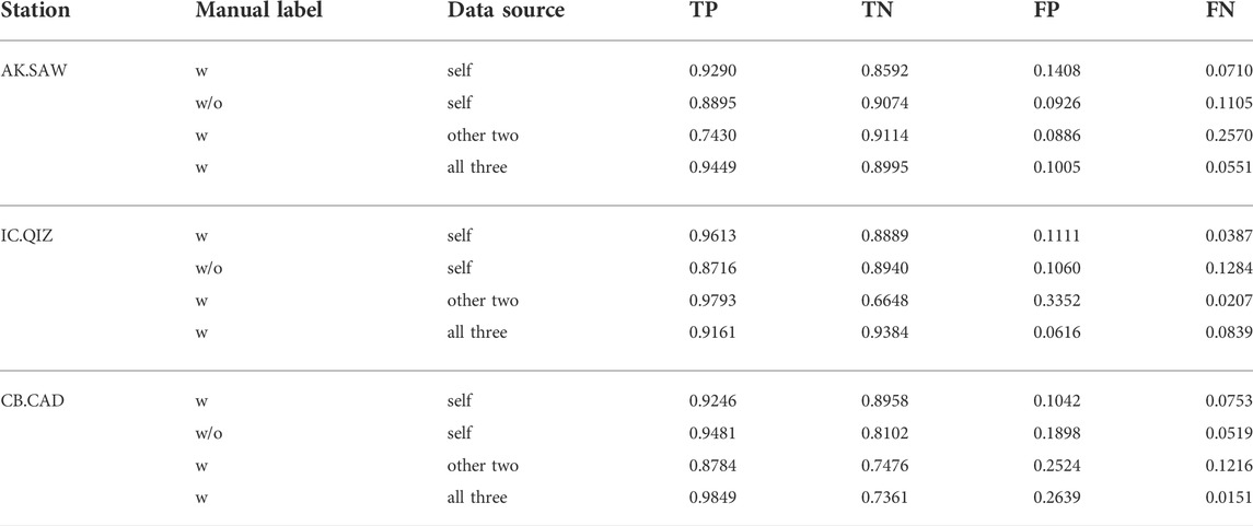
TABLE 3. Normalized confusion matrixes of the CNN-BiLSTM model used with or without manually labeled datasets from station itself, other two stations, or all the three stations. W means training set with manual labels and w/o means training set without manual labels.

Besides using noisy datasets labeled automatically by traditional methods, one may wonder if a large receiver function dataset can solve the training set problem. As the receiver function is related to the relative response of Earth structure near the receiver, one obvious worry is that mixing data from different stations with different geological backgrounds could cause a negative effect. To address this concern, we conduct the following experiments: 1) use the data from all the three stations together to train the model (Supplementary Figures S11) and calculate its confusion matrix (Table 3); 2) use the label from the other two stations to train the model for each station (Supplementary Figures S12 and Table 3). The results show that mixing receiver functions from different stations together for training improves the model’s performance on the AK. SAW station and shows no notable negative influence on the other two stations. All models trained with data from the other two stations have low accuracy, suggesting the background information on local Earth structures has a significant impact on this task. Overall, there is still a great need for constructing regional-scale or global-scale receiver function datasets, similar to earthquake detection and phase picking datasets (Mousavi et al., 2019), to further improve deep-learning enabled receiver function analysis.

In summary, we first compare four different model designs of deep learning to select the best model for receiver function quality control. The CNN-BiLSTM model achieves the best performance on the training and validation datasets. Our study suggests early stopping is crucial in easing the overfitting issue for receiver function quality control. The BiLSTM layer could further improve the performance, while the transformer layer may not suit small dataset scenarios. We then test the potential of our method on earthquakes with magnitudes between 5.0 and 5.5 and compare the stacked waveforms and H-κ stacking results to validate its performance. Finally, we discuss how to tackle the lack of training set by: 1) showing that the deep learning model can directly learn from noisy labels by traditional methods and produce better quality control results; 2) comparing the models trained with receiver functions of different station combinations.

The advantages of the proposed quality control method include: 1) It can process extensive receiver function data automatically, rapidly, and accurately; 2) By mining high-quality receiver functions from earthquakes with magnitudes between 5.0 and 5.5, it can provide better back-azimuth coverage and a wider distribution of piercing points, enabling fine dipping and anisotropic structural imaging at single stations, especially for those with short observation durations; 3) It can directly learn from noisy labels by traditional automatic methods as a substitute for a high-quality manually labeled dataset; 4) The proposed method may extend to the S-wave receiver function and P-wave transverse receiver function in the case of labeled datasets, as no a priori knowledge about the P-wave radial receiver function is used during training the deep learning model.

The limitations of our method include: 1) the accuracy of models trained using noisy data is slightly lower than those trained on manually labeled datasets. This issue may be addressed by constructing a high-quality regional-scale or global-scale receiver function dataset; 2) different methods and parameters used in receiver function calculation could result in different input waveforms. Hence, these factors must be kept consistent during the training, examination, and application of the deep learning model.

Conclusion

We study the impact of different deep learning model designs on receiver function quality control. We propose a model that combines CNN and LSTM layers. Our model achieves human-level performance on the earthquake dataset with magnitudes above 5.5 and outperforms the traditional method on the earthquake dataset with magnitudes between 5.0 and 5.5. Our study provides an accurate and fully automated approach for receiver function quality control and a powerful tool for making use of small earthquakes that have been long ignored in previous studies.

Data availability statement

Publicly available datasets were analyzed in this study. This data can be found here: https://github.com/gongchang96/Receiver-Function-Quality-Control.

Author contributions

CG conducted the research, plotted the figures, and wrote the manuscript. ZX helped in developing the code. XW helped in H-k stacking. LC and CG contributed to the conception and design of the study. All authors contributed to manuscript revision, read, and approved the submitted version.

Funding

This study is financially supported by the National Natural Science Foundation of China (Grant 42288201) and the Strategic Priority Research Program (A) of Chinese Academy of Sciences (Grant No. XDA20070302).

Acknowledgments

We thank the Handling Editor and two reviewers for their constructive comments and suggestions, which significantly improved the manuscript. We thank the researchers who developed and shared Obspy (Krischer et al., 2015) and HiPerSeis (Hassan et al., 2020), which are used for data processing and analysis. We use TensorFlow framework to build and train deep learning models (Abadi et al., 2016). The figures are generated using Generic Mapping Tools (GMT) (Wessel and Smith, 1998) and Matplotlib (Hunter, 2007). The data from station AK.SAW are obtained from the University of Alaska Fairbanks (Alaska Earthquake Center, Univ. of Alaska Fairbanks, 1987). The data from station CB.CAD and station IC.QIZ are obtained from Data Management Centre of China National Seismic Network at Institute of Geophysics (SEISDMC, doi:10.11998/SeisDmc/SN), China Earthquake Networks Center. The transformer implementation is based on EQTransformer (Mousavi et al., 2020; https://github.com/smousavi05/EQTransformer). The quality control method workflow and trained deep learning models are publicly available on GitHub at https://github.com/gongchang96/Receiver-Function-Quality-Control.

Conflict of interest

The authors declare that the research was conducted in the absence of any commercial or financial relationships that could be construed as a potential conflict of interest.

Publisher’s note

All claims expressed in this article are solely those of the authors and do not necessarily represent those of their affiliated organizations, or those of the publisher, the editors and the reviewers. Any product that may be evaluated in this article, or claim that may be made by its manufacturer, is not guaranteed or endorsed by the publisher.

Supplementary material

The Supplementary Material for this article can be found online at: https://www.frontiersin.org/articles/10.3389/feart.2022.921830/full#supplementary-material

Supplementary Figure S1 | Location of stations (triangle) and distribution of teleseismic events (circles) used in this study. (A) Location of station AK.SAW (triangle) and distribution of 5456 events (circles) in the training and validation dataset with magnitudes larger than 5.5. (B) Location of station AK.SAW (triangle) and distribution of 14398 events (circles) in the training and validation dataset with magnitudes between 5.0 and 5.5. (C) Location of station IC.QIZ (triangle) and distribution of 5319 events (circles) in the training and validation dataset with magnitudes larger than 5.5. (D) Location of station IC.QIZ (triangle) and distribution of 24551 events (circles) in the training and validation dataset with magnitudes between 5.0 and 5.5. (E) Location of station IC.QIZ (triangle) and distribution of 1712 events (circles) in the training and validation dataset with magnitudes larger than 5.5. (F) Location of station IC.QIZ (triangle) and distribution of 1857 events (circles) in the training and validation dataset with magnitudes between 5.0 and 5.5.

Supplementary Figure S2 | Diagrams (A–C) and training and validation loss (D–F) of the three FC models with different hidden layers. (A,D) FC model with 2 hidden layers. (B,E) FC model with 3 hidden layers. (C,F) FC model with 4 hidden layers.

Supplementary Figure S3 | Receiver functions from station AK.SAW with magnitudes above 5.5 stacked in each back-azimuth bin (A–D). (A) Quality control by FC Model. (B) Quality control by CNN model. (C) Quality control by CNN-BiLSTM Model. (D) Quality control by CNN-BiLSTM-Trans Model.

Supplementary Figure S4 | Receiver functions from station IC.QIZ with magnitudes above 5.5 stacked in each back-azimuth bin (A–D). (A) Quality control by FC Model. (B) Quality control by CNN model. (C) Quality control by CNN-BiLSTM Model. (D) Quality control by CNN-BiLSTM-Trans Model.

Supplementary Figure S5 | Receiver functions from station CB.CAD with magnitudes above 5.5 stacked in each back-azimuth bin (A–D). (A) Quality control by FC Model. (B) Quality control by CNN model. (C) Quality control by CNN-BiLSTM Model. (D) Quality control by CNN-BiLSTM-Trans Model.

Supplementary Figure S6 | The receiver function waveforms from station AK.SAW around a polar plot with the source direction. Red lines are the average waveforms of many similar waveforms in back-azimuth bins. (A) Manually quality controlled dataset containing 941 receiver functions with earthquake magnitudes larger than 5.5. (B) Automatically quality controlled dataset by the CNN-BiLSTM model containing 691 receiver functions with earthquake magnitudes between 5.0 and 5.5. (C) Automatically quality controlled dataset by the traditional method in HiPerSeis containing 95 receiver functions with earthquake magnitudes between 5.0 and 5.5.

Supplementary Figure S7 | The receiver function waveforms from station IC.QIZ around a polar plot with the source direction. Red lines are the average waveforms of many similar waveforms in back-azimuth bins. (A) Manually quality controlled dataset containing 771 receiver functions with earthquake magnitudes larger than 5.5. (B) Automatically quality controlled dataset by the CNN-BiLSTM model containing 686 receiver functions with earthquake magnitudes between 5.0 and 5.5. (C) Automatically quality controlled dataset by the traditional method in HiPerSeis containing 74 receiver functions with earthquake magnitudes between 5.0 and 5.5.

Supplementary Figure S8 | The receiver function waveforms from station CB.CAD around a polar plot with the source direction. Red lines are the average waveforms of many similar waveforms in back-azimuth bins. (A) Manually quality controlled dataset containing 964 receiver functions with earthquake magnitudes larger than 5.5. (B) Automatically quality controlled dataset by the CNN-BiLSTM model containing 458 receiver functions with earthquake magnitudes between 5.0 and 5.5. (C) Automatically quality controlled dataset by the traditional method in HiPerSeis containing 265 receiver functions with earthquake magnitudes between 5.0 and 5.5.

Supplementary Figure S9 | Stacked receiver functions against the epicentral distance. Grey lines show the theoretical arrival times of the converted phase and multiple phase from the Moho based on the results of H-κ stacking. (A) Manually quality controlled station AK.SAW dataset with earthquake magnitudes larger than 5.5. (B) Automatically quality controlled station AK.SAW dataset by the CNN-BiLSTM model with earthquake magnitudes between 5.0 and 5.5. (C,D) are the same as (A,B) but for station IC.QIZ datasets. (E,F) are the same as (A,B) but for station CB.CAD datasets.

Supplementary Figure S10 | Training and validation loss of the CNN-BiLSTM model used training set labeled by the traditional method (HiPerSeis). (A) Station AK.SAW dataset. (B) station IC.QIZ dataset. (C) Station CB.CAD dataset.

Supplementary Figure S11 | Training and validation loss of the CNN-BiLSTM model used manually labeled training set from all the three stations (AK.SAW, IC.QIZ, and CB.CAD).

Supplementary Figure S12 | Training and validation loss of the CNN-BiLSTM model used manually labeled training set from two stations. (A) Using training set from station IC.QIZ and station CB.CAD. (B) Using training set from station AK.SAW and station CB.CAD. (C) Using training set from station IC.QIZ and station CB.CAD.

Supplementary Table S1 | Normalized confusion matrixes of the FC models with different hidden layers.

Supplementary Table S2 | Normalized confusion matrixes of the traditional method with different distance thresholds on station AK.SAW dataset (magnitude > 5.5).

References

Abadi, M., Barham, P., Chen, J., Chen, Z., Davis, A., Dean, J., et al. (2016). “TensorFlow: A system for large-scale machine learning,” in Proceedings of the 12th USENIX Conference on Operating Systems Design and Implementation, Savannah, Georgia, November 2–4, 2016, 265–283. Available at: https://www.usenix.org/system/files/conference/osdi16/osdi16-abadi.pdf.

Google Scholar

Alaska Earthquake Center, Univ. of Alaska Fairbanks (1987). Alaska regional network [data set]. Fairbanks: International Federation of Digital Seismograph Networks. doi:10.7914/SN/AK

CrossRef Full Text | Google Scholar

Chen, Y., Niu, F., Liu, R., Huang, Z., Tkalčić, H., Sun, L., et al. (2010). Crustal structure beneath China from receiver function analysis. J. Geophys. Res. 115 (B3), B03307. doi:10.1029/2009JB006386

CrossRef Full Text | Google Scholar

D’Ascoli, S., Touvron, H., Leavitt, M. L., Morcos, A. S., Biroli, G., and Sagun, L. (2021). “ConViT: Improving vision transformers with soft convolutional inductive biases,” in Proceedings of the 38th international conference on machine learning. Editors M. Meila, and T. Zhang (PMLR), 139, 2286–2296.

Google Scholar

Devlin, J., Chang, M.-W., Lee, K., and Toutanova, K. (2019). “{BERT}: Pre-training of deep bidirectional transformers for language understanding,” in Proceedings of the 2019 Conference of the North {A}merican Chapter of the Association for Computational Linguistics: Human Language Technologies, Minneapolis, Minnesota, June 2–7, 2019 (Minneapolis, Minnesota: Association for Computational Linguistics), 4171–4186. (Long and Short Papers). doi:10.18653/v1/N19-1423

CrossRef Full Text | Google Scholar

Dosovitskiy, A., Beyer, L., Kolesnikov, A., Weissenborn, D., Zhai, X., Unterthiner, T., et al. (2020). An image is worth 16x16 words: Transformers for image recognition at scale. Available at: https://arxiv.org/abs/2010.11929.

Google Scholar

Gan, L., Wu, Q., Huang, Q., and Tang, R. (2021). Quick selection of receiver function based on convolutional neural network. Chin. J. Geophys. 64 (7), 2394–2404. doi:10.6038/cjg2021O0141

CrossRef Full Text | Google Scholar

Gao, S. S., and Liu, K. H. (2014). Mantle transition zone discontinuities beneath the contiguous United States. J. Geophys. Res. Solid Earth 119 (8), 6452–6468. doi:10.1002/2014JB011253

CrossRef Full Text | Google Scholar

Hassan, R., Hejrani, B., Zhang, F., Gorbatov, A., and Medlin, A. (2020). High-performance seismological tools (HiPerSeis). Geosci. Aust. doi:10.11636/135095

CrossRef Full Text | Google Scholar

He, K., Zhang, X., Ren, S., and Sun, J. (2016). “Deep residual learning for image recognition,” in 2016 IEEE Conference on Computer Vision and Pattern Recognition (CVPR), Las Vegas, NV, USA, 27-30 June 2016, 770–778. doi:10.1109/CVPR.2016.90

CrossRef Full Text | Google Scholar

Hochreiter, S., and Schmidhuber, J. (1997). Long short-term memory. Neural Comput. 9, 1735–1780. doi:10.1162/neco.1997.9.8.1735

PubMed Abstract | CrossRef Full Text | Google Scholar

Hunter, J. D. (2007). Matplotlib: A 2D graphics environment. Comput. Sci. Eng. 9, 90–95. doi:10.1109/MCSE.2007.55

CrossRef Full Text | Google Scholar

Kong, Q., Trugman, D., Ross, Z., Bianco, M., Meade, B., and Gerstoft, P. (2018). Machine learning in seismology: Turning data into insights. Seismol. Res. Lett. 90 (1), 3–14. doi:10.1785/0220180259

CrossRef Full Text | Google Scholar

Krischer, L., Megies, T., Barsch, R., Beyreuther, M., Lecocq, T., Caudron, C., et al. (2015). ObsPy: A bridge for seismology into the scientific Python ecosystem. Comput. Sci. Discov. 8 (1), 014003. doi:10.1088/1749-4699/8/1/014003

CrossRef Full Text | Google Scholar

LeCun, Y., Bengio, Y., and Hinton, G. (2015). Deep learning. Nature 521 (7553), 436–444. doi:10.1038/nature14539

PubMed Abstract | CrossRef Full Text | Google Scholar

Li, Z., Tian, Y., Zhao, P., Liu, C., and Li, H. (2021). Receiver functions auto-picking method on the basis of deep learning. Chin. J. Geophys. (in Chinese) 64 (5), 1632–1642. doi:10.6038/cjg2021O0378

CrossRef Full Text | Google Scholar

Ligorría, J. P., and Ammon, C. J. (1999). Iterative deconvolution and receiver-function estimation. Bull. Seismol. Soc. Am. 89 (5), 1395–1400. doi:10.1785/bssa0890051395

CrossRef Full Text | Google Scholar

Miller, M. S., O’Driscoll, L. J., Porritt, R. W., and Roeske, S. M. (2018). Multiscale crustal architecture of Alaska inferred from P receiver functions. Lithosphere 10 (2), 267–278. doi:10.1130/l701.1

CrossRef Full Text | Google Scholar

Mousavi, S. M., Ellsworth, W. L., Zhu, W., Chuang, L. Y., and Beroza, G. C. (2020). Earthquake transformer—An attentive deep-learning model for simultaneous earthquake detection and phase picking. Nat. Commun. 11 (1), 3952–4012. doi:10.1038/s41467-020-17591-w

PubMed Abstract | CrossRef Full Text | Google Scholar

Mousavi, S. M., Sheng, Y., Zhu, W., and Beroza, G. C. (2019). STanford EArthquake dataset (STEAD): A global data set of seismic signals for AI. IEEE Access 7, 179464–179476. doi:10.1109/ACCESS.2019.2947848

CrossRef Full Text | Google Scholar

Munch, F. D., Khan, A., Tauzin, B., van Driel, M., and Giardini, D. (2020). Seismological evidence for thermo-chemical heterogeneity in Earth's continental mantle. Earth and Planetary Science Letters 539, 116240. doi:10.1016/j.epsl.2020.116240

CrossRef Full Text | Google Scholar

Rolnick, D., Veit, A., Belongie, S., and Shavit, N. (2017). Deep learning is robust to massive label noise. Available at: https://arxiv.org/abs/1705.10694#:∼:text=Deep%20neural%20networks%20trained%20on,image%20classification%20and%20other%20tasks.

Google Scholar

Schulte-Pelkum, V., Monsalve, G., Sheehan, A., Pandey, M. R., Sapkota, S., Bilham, R., et al. (2005). Imaging the Indian subcontinent beneath the himalaya. Nature 435 (7046), 1222–1225. doi:10.1038/nature03678

PubMed Abstract | CrossRef Full Text | Google Scholar

Shen, W., Ritzwoller, M. H., Schulte-Pelkum, V., and Lin, F.-C. (2012). Joint inversion of surface wave dispersion and receiver functions: A bayesian monte-carlo approach. Geophys. J. Int. 192 (2), 807–836. doi:10.1093/gji/ggs050

CrossRef Full Text | Google Scholar

Tauzin, B., Debayle, E., and Wittlinger, G. (2010). Seismic evidence for a global low-velocity layer within the Earth’s upper mantle. Nat. Geosci. 3 (10), 718–721. doi:10.1038/ngeo969

CrossRef Full Text | Google Scholar

Vaswani, A., Shazeer, N., Parmar, N., Uszkoreit, J., Jones, L., Gomez, A. N., et al. (2017). “Attention is all you need,” in Proceedings of the 31st International Conference on Neural Information Processing Systems, Long Beach, California, December 4–9, 2017 (Red Hook, NY, USA: Curran Associates Inc), 6000–6010.

Google Scholar

Wei, Z., Chen, L., Li, Z., Ling, Y., and Li, J. (2016). Regional variation in Moho depth and Poisson’s ratio beneath eastern China and its tectonic implications. Journal of Asian Earth Sciences 115, 308–320. doi:10.1016/j.jseaes.2015.10.010

CrossRef Full Text | Google Scholar

Wessel, P., and Smith, W. H. F. (1998). New, improved version of generic mapping tools released. Eos Trans. AGU. 79, 579. doi:10.1029/98EO00426

CrossRef Full Text | Google Scholar

Yang, X., Pavlis, G. L., and Wang, Y. (2016). A quality control method for teleseismic P-wave receiver functions. Bulletin of the Seismological Society of America 106 (5), 1948–1962. doi:10.1785/0120150347

CrossRef Full Text | Google Scholar

Zhou, Y., Ghosh, A., Fang, L., Yue, H., Zhou, S., and Su, Y. (2021). A high-resolution seismic catalog for the 2021 ms6.4/mw6.1 YangBi earthquake sequence, yunnan, China: Application of AI picker and matched filter. Earthquake Science 34, 1–9. doi:10.29382/eqs-2021-0031

CrossRef Full Text | Google Scholar

Zhu, L., and Kanamori, H. (2000). Moho depth variation in southern California from teleseismic receiver functions. J. Geophys. Res. 105 (B2), 2969–2980. doi:10.1029/1999JB900322

CrossRef Full Text | Google Scholar