Changes in the Runoff of Urumqi Glacier No. 1 Under Climate Change: From Historical Observation to Future Prediction

This study explores the ice volumes of Urumqi Glacier No. 1 from 2013 to 2112 to examine the changes in the runoff of the glacier. Based on the Sixth Assessment Report of the Intergovernmental Panel on Climate Change (IPCC), the changes of the glacier were predicted under three hypothetical climate scenarios: SSP1-1.9, SSP2-4.5, and SSP5-8.5 scenarios. The results derived from the Elmer/Ice ice-flow model showed increasing runoff till 2040 in the SSP2-4.5 and SSP5-8.5 scenarios and gradually decreasing runoff in the SSP1-1.9 scenario. The glacier areas and ice volumes of the two branches will keep declining under all the climate scenarios, including fast reductions until 2080 and slow reductions by the end of the ablation period. Moreover, the east branch (EB) will disappear at the end of the 21st century under the SSP2-4.5 and SSP5-8.5 scenarios. With much mass loss of the EB under all the climate scenarios, the runoff will increase in the early 100-year period and decrease until it is being infinitely close to the precipitation, which is similar with that of the west branch (WB). Since 2070, the ice volumes of the WB will contribute more than 50% of the whole glacier volumes under all the climate scenarios. The WB ice volume percentage will reach 100% in 2080 for the disappearance of the EB under the SSP5-8.5 scenario. As the fast retreat of the EB before 2080, the variations of the total runoff will be consistent with that of the EB runoff, and the EB runoff will account for more than 60% of the total runoff before 2070 under all the climate scenarios. Even if the meltwater of Urumqi Glacier No. 1 is stable from the late 21st century (after 2090), it will decline to approximately 15% of that in 2013. It will greatly influence the runoff of Urumqi River, hence human life and biodiversity.

1 Introduction

Mountain and polar glaciers are committed to continue melting for decades or centuries under the unequivocal warming of the climate system, and five representative climate scenarios in the Sixth Assessment Report of IPCC are shown in Table 1 (IPCC, 2021). Glaciers in high mountain regions are expected to lose substantial mass by the end of the 21st century (Zemp et al., 2015; Kraaijenbrink et al., 2017; Pörtner et al., 2019), though the accelerating trend of mass loss has appeared during the past two or three decades (Haeberli et al., 2000; Barry, 2006; Li et al., 2011a). As a small glacier will typically respond faster than a larger glacier to climate change (Bahr et al., 1998), studying mass balances of high-mountain glaciers much smaller than the polar ice sheets is of great value. Moreover, the meltwater from glaciers on high mountains is the lifeline for local and downstream residents, which can influence local economy and ecosystems (Ding et al., 2006; Immerzeel et al., 2010; Li et al., 2010; Ren et al., 2017; Gao et al., 2018).

TABLE 1

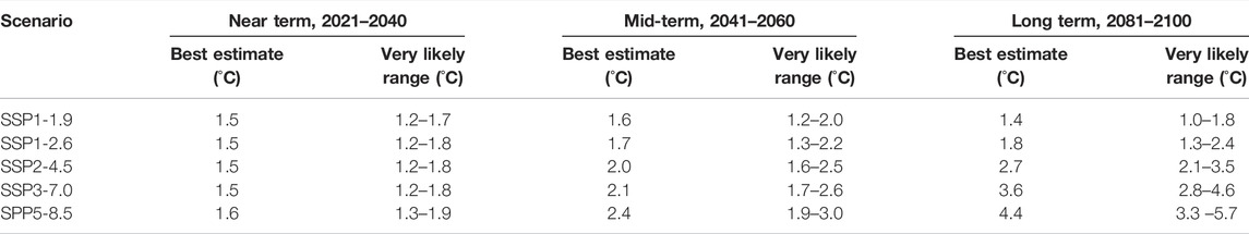
TABLE 1. The climate scenarios in the Sixth Assessment Report of IPCC.

Urumqi Glacier No. 1 is a reference glacier with a long data series, important location, and significant local water supply in the Word Glacier Monitoring Service (WGMS) network (Zemp et al., 2009; Li et al., 2011b). The glacier is located in the Tianshan mountains in the arid and semi-arid regions of Eurasia (Figure 1), which is surrounded by vast deserts and the Gobi (Yue et al., 2021). The acceleration of mass loss occurred in 1985 and 1996, mainly due to the increases in temperature during the melting period, the ice temperature augment, and the decrease in the albedo of glacier surfaces (Li et al., 2011b). Furthermore, the enhanced glacier melting by summer climate warming and annual precipitation augmenting made the annual basin runoff significantly increase in the past 45 years (Ye et al., 2005; Sun et al., 2013). In 1993, Urumqi Glacier No. 1 separated to the EB and WB, but the two branches of the Glacier still experienced the same warming scenario. However, WB was considered to be more sensitive to the recent climate change for its larger slopes and smaller glacier areas (Xu et al., 2011).

FIGURE 1

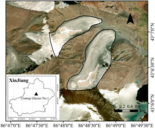
FIGURE 1. Geographic location of Urumqi Glacier No. 1, Tianshan mountain, and the black triangle in the map of Xinjiang indicated the location of the study area. The image of the glacier was obtained by field measurement.

In-situ measurements were used to study the changes of Urumqi Glacier No. 1. The mass balance of Urumqi Glacier No. 1 has been measured since 1959 by the glaciological method using ablation stakes and snow pits except during the 1967–1979 period when the observations were interrupted (Wang et al., 2014). Terrestrial laser scanning measurements were used to monitor glacier boundaries, annual elevation changes, and geodetic mass balance in Urumqi Glacier No. 1 from 2015 to 2017 (Xu et al., 2019). The ice thickness of the glacier was detected by the ground penetrating radar (GPR) and the maximum thickness was on the mainstream line, more than 100 m in 2001 (Sun et al., 2003). Moreover, the max ice-flow velocity of Urumqi Glacier No. 1 could reach 0.75 m·m⁻¹ from May to July in 2017, and the velocity variations were influenced by glacier thickness, glacier slopes, terrains of bedrocks, and glacier ice temperatures (Zhou et al., 2009).

How Urumqi Glacier No. 1 will evolve in the future under climate change can affect the amount of the headwaters of the Urumqi River, because the melt water from Urumqi Glacier No. 1 accounts for about 70% of the water that feeds the headwaters (Yang, 1991; Jia et al., 2019). Therefore, the Elmer/Ice ice-flow model was used to simulate the evolution of Urumqi Glacier No. 1 to the end of the 21st century, which could project the changes in runoff at the headwaters of the Urumqi River.

2 Data and Methods

2.1 Data

2.1.1 DEMs of Urumqi Glacier No. 1

The DEMs included the surface DEM and the bedrock DEM of Urumqi Glacier No. 1 in 2012. A radar dataset along the mainstream and seven (six) transverse lines of the EB (WB) was collected to get the ice thickness by using a pulseEKKO PRO GPR system with a high frequency of 100 MHz, and this GPR system was made by Sensors & Software Inc. (Canada). The surface DEM was obtained from real-time kinematic measurements by interpolation, and the bedrock DEM was obtained by subtracting the ice thickness from the surface DEM. The pixel resolutions of DEMs were 10 m, shown in Figure 2.

FIGURE 2

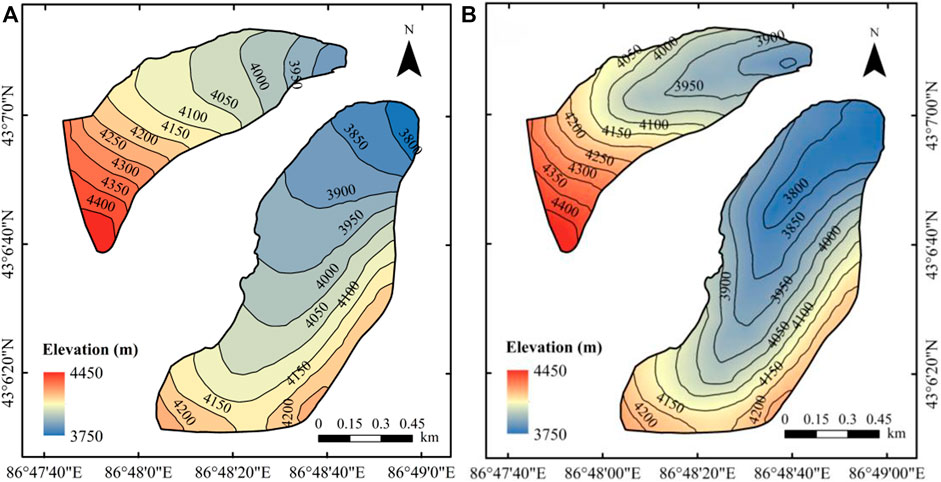
FIGURE 2. (A) Surface and (B) bedrock DEMs of Urumqi Glacier No. 1 and the contour intervals both are 50 m.

2.1.2 In-situ Measured Data

The surface ice-flow velocities were acquired by repeated GPS measurement via stakes, with 22 stakes in EB and 19 stakes in WB (Figure 3). To reduce the impact of accident errors, we calculated the averages of ice-flow velocities from 2010 to 2016 as the initial velocities in the simulation (Table 2), and the maximum ice-flow velocity was found along the mainstream lines at the point E2 (EB) and the point F2 (WB). The measurements of the glacier mass balance were also derived from these stakes.

FIGURE 3

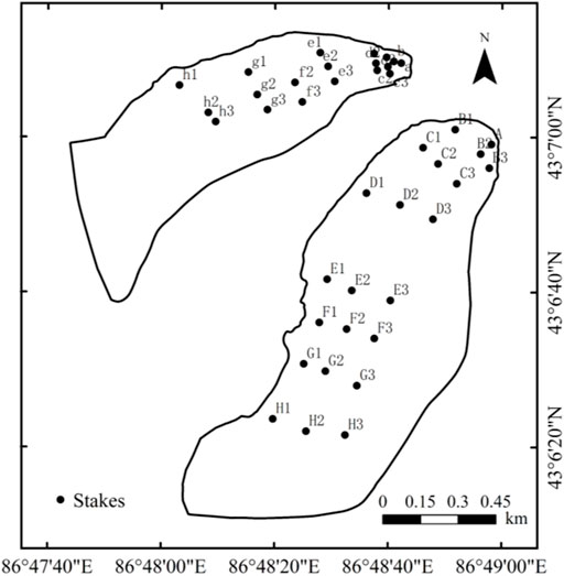
FIGURE 3. The locations of stakes on the glacier surface.

TABLE 2

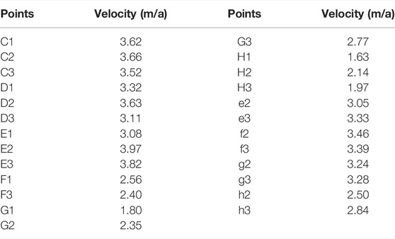
TABLE 2. The averages of measured ice-flow velocities from 2010 to 2016 of Urumqi Glacier No. 1.

The stakes on the glacier were also taken in the use of measuring the net surface mass balance (SMB) of the glacier (Li and Wang, 2016) from 2006 to 2012 (Figure 4). The net mass balance increased with elevation, and the gradients in Figure 4 varied in different elevations. Moreover, the gradients with the net mass balance larger than 0 were close to 0.

FIGURE 4

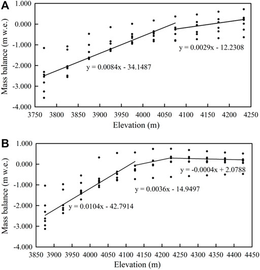
FIGURE 4. The mass balance measurements of Urumqi Glacier No. 1’s (A) EB and (B) WB from 2006 to 2012, where the line is the fitted value in ablation or accumulation area.

Being sensitive to the air temperature, the equilibrium line altitude (ELA) was an important parameter of the SMB. According to the observations and the researches about the ELA of Urumqi Glacier No. 1, the initial ELA (ELA₀) of the EB was selected as 4,075 m (Dong et al., 2012; Li et al., 2013), and the initial ELA of the WB was about 45 m higher than that of the EB (Xu et al., 2011; Xia et al., 2012; Li and Wang, 2016). The SMB gradient is shown in Figure 4 by dividing into ablation area and accumulation area based on the observations.

The borehole ice temperatures were detected from the 50 m deep borehole at 3,850 m on EB during January 2010 to October 2011. The active layer was obvious within the 16 m depth where the ice temperature was −4.39°C in Figure 5.

FIGURE 5

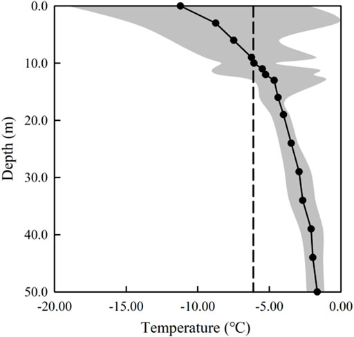
FIGURE 5. The borehole ice temperatures from a depth of 50 m. The points showed the average ice temperature during January 2010 to October 2011, the shadow showed the fluctuation ranges of annual ice temperature, and the dashed line is the local average air temperature.

The precipitations were observed at the Daxigou meteorological station from 1959 to 2019 (Figure 6), which were used to calculate the future runoff in our simulations.

FIGURE 6

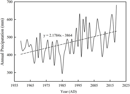
FIGURE 6. The annual precipitation data from the Daxigou meteorological station. The solid line denotes the measured annual precipitation from 1959 to 2019. The dashed line is the linear fit of the annual precipitation.

2.2 Methods

2.2.1 Ice Volume

Glacier was the resource and “solid reservoir” that reflected the capacity of water storage. The ice volume changes in the future could be analyzed by the ice thickness, and the ice volume of Urumqi Glacier No. 1 could be computed by multiplying the thickness by the area as follows:

$Volum{e}_i={\displaystyle \sum \left(dept{h}_i\times S\right)}(1)$

where depth_i was the glacier depth every pixel of the ith year from 2012 and S was the pixel resolution.

2.2.2 Glacier Runoff

The glacier runoff consisted of the annual precipitation and the meltwater. The annual precipitation was obtained by multiplying the total precipitation by the glacier area, and the precipitation in the future was assumed to increase according to the curve in Figure 6, while the meltwater was the mass loss of the glacier in a year.

The mass loss of the glacier was a part of the SMB which was the algebraic sum of the accumulation from the solid precipitation and the ablation from glacier melt in the glacier surface at unit time (Qin et al., 2016). The sensitivity of ELA to temperature, α, was 61.7 m/°C, that meant the glacier ELA ascended (descended) 61.7 m when the air temperature increased (decreased) by 1°C (Dong et al., 2012), hence, the ELA in the ith year from 2012 and the meltwater were calculated as below (Ai et al., 2019):

$EL{A}_i=EL{A}_0+\alpha \mathrm{\Delta }{T}_i(2)$

$Meltwate{r}_i={\displaystyle \sum \left[\left(Z{s}_i-EL{A}_i\right)\times SMB\left(Zs\right)\times S\right]}(3)$

where ΔT_i was the temperature change of the ith year relative to 2012, Zs_i was ice surface elevation, ELA_i was the ELA of the ith year from 2012, and S was the pixel resolution.

Therefore, taking the precipitation into consideration, the glacier runoff could be calculated:

$Runof{f}_i=Meltwate{r}_i+Precipitatio{n}_i(4)$

2.2.3 Elmer/Ice Ice-Flow Model

Elmer/Ice is a full-Stokes, finite element, and ice-sheet/ice-flow model, which can be used to simulate the evolution of the mountain glacier and Antarctic ice sheet (Zhao et al., 2014; Zhang et al., 2017).

Ice is incompressible fluid and its flow meets with Stokes equations:

$\text{div}\mathit{u}=0(5)$

$\text{div}\tau -\text{grad}p+\text{ρ}g=\text{0}(6)$

where u is the ice-flow velocity, τ is the deviatoric stress tensor, p is the ice pressure, g is the gravitational acceleration, and ρ is the ice density.

The deviatoric stress τ and the strain rate $\dot{\epsilon }$ equation satisfy Glen’s law:

$\tau =2\eta \dot{\epsilon }(7)$

where the effective viscosity η is defined as:

$\eta =\frac{1}{2}{\left(EA\right)}^{-\frac{1}{n}}{\dot{\epsilon }}_e^{\left(1-n\right)/n}(8)$

where ${\dot{\epsilon }}_e^2=tr\left({\dot{\epsilon }}^2\right)$ is the square of the second invariant of the strain rate, E is the Glen enhancement factor, and n is the Glen exponent. A is a rheological parameter depending on the ice temperature relative to the pressure melting point, T′:

$A\left(T^{\prime }\right)=A_0{e}^{-\frac{Q}{\left(R{T}^{\prime }\right)}}(9)$

where A₀ is the rate factor, Q is the creep activation energy, and R is the gas constant.

There is a basal sliding of the Urumqi Glacier No. 1 and the basal boundary condition can be expressed as follows:

${\tau }_b=\beta u_b(10)$

where τ_b is the basal shear stress, β is the basal friction parameter, and u_b is the basal tangential velocity.

The equation of Zs changes with time as follows:

$\frac{\partial Zs}{\partial t}+u_x\frac{\partial Zs}{\partial x}+u_y\frac{\partial Zs}{\partial y}-u_z=SMB(11)$

where u_x, u_y, and u_z are the three components of ice-flow velocity in the three directions x, y, and z, respectively.

The parameters of the ice-flow model in this study are shown in Table 3 (Wang et al., 2019).

TABLE 3

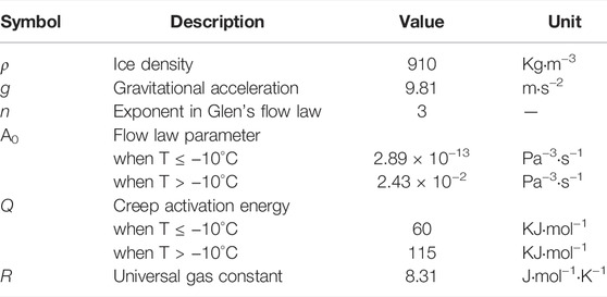
TABLE 3. The parameters of the ice-flow model.

2.2.4 Simulation Process

There were two phases of the simulation process: the steady-state simulation (diagnostic simulation) constrained by GPS data was performed and mainly obtained two important parameters: the basal friction parameter β and the Glen enhancement factor E; and the transient simulation mainly predicted the evolution of Urumqi Glacier No. 1 using the steady-state simulation result as the initial condition.

In the steady-state simulation, the stakes with secure GPS records were chosen to calculate to horizontal ice-flow velocities, and the measured velocities were used to constrain the simulation velocities by adjusting two important parameters in the model—β and E. In the model, β was the basal friction parameter and E was the Glen enhancement factor.

Our adjustment of the parameters was in four processes (Figure 7A).

① E was assigned an appropriate value when β took a certain value, and the combination of β and E was used to make simulated velocity match well with the maximum measured velocity at point E2. According to the minimum of the residual sum of squares in Table 4, we chose β = 0.01 and E = 0.003.

② As the parameters we chose indicated that the simulated velocities above 3,950 m were much higher than the measured velocities, we adjusted the β above 3,950 m to be larger than 0.01; thus, the basal friction parameter β above 3,950 m was defined as β₂ and the β in other palaces was β₁. As the β₂ larger than 0.03 made the simulated velocities much lower than the measured velocities, we chose β₂ = 0.02 or β₂ = 0.03 to do further adjustment.

③ When β₂ was 0.02 or 0.03, all the simulated velocities were lower than the measured velocities, so we made E larger than 0.003 and found that the value of 0.05 made the simulated velocities closer to the measured results.

④ In the third process, with β₁ = 0.01, β₂ = 0.03, and E = 0.05, the simulated velocities below 3,950 m were much higher than the measured velocities, so we adjusted β₁ to 0.02 and 0.015. Comparing the results in the fourth process, we chose the best result—β₁ = 0.015, β₂ = 0.03, and E = 0.05.

FIGURE 7

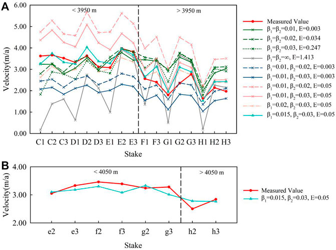
FIGURE 7. Simulated results of the EB and the WB for the sliding states. (A) Measured velocities, full sliding, no sliding, and partial sliding at the glacier base results of the EB, and the black dashed line denotes the elevation of 3,950 m; (B) Measured velocities, partial sliding at the glacier base simulation results of the WB, and the black dashed line denotes the elevation of 4,050 m.

TABLE 4

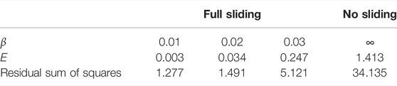
TABLE 4. Residual sum of squares of the difference between the measured and simulated velocities below 3,950 m.

Taking the aforementioned parameters, we got the simulated velocities matching well with the measured velocities in the EB (Figure 7A, Figure 8A). As for the two parameters of the WB, the value of elevation, 4,050 m, was used to differentiate β and E, and the simulated velocities matched well with the measured velocities, too (Figure 7B, Figure 8B).

FIGURE 8

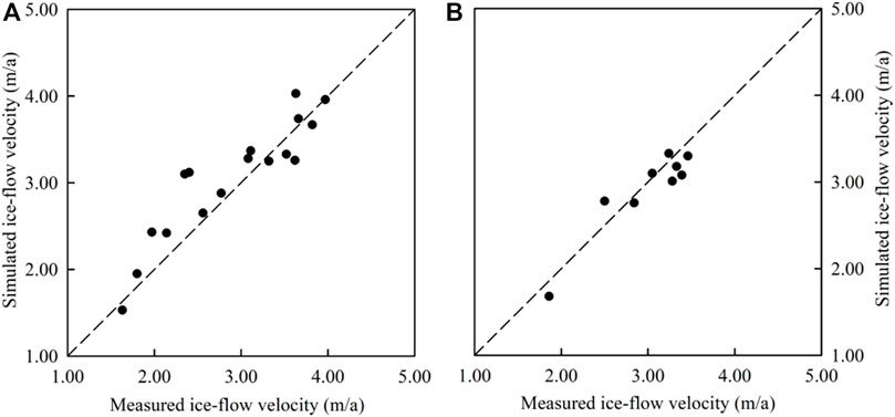
FIGURE 8. Error graphs of (A) the EB and (B) the WB using the best estimates of the model parameters. The black points denote ice-flow velocities at the stakes depicted in Figure 3. The dashed line denoted the states when the measured ice-flow velocities were equal to the simulated ice-flow velocities.

In the transient-state simulation, three warming scenarios in IPCC were chosen (SSP1-1.9, SSP2-4.5, and SSP5-8.5) in Table 1. In the three climate scenarios, the air temperature would increase 0.014°C·a⁻¹, 0.027°C·a⁻¹ and 0.044°C·a⁻¹, respectively (Table 5). The ELA of the glacier was also increased per year based on the Eq. 2 and the SMB gradient was shown in Figure 4 based on the observations. Under the three hypothetical climate scenarios, we predicted the evolution of the glacier in 100 years (2013–2112).

TABLE 5

TABLE 5. The increased air temperature per year.

The ice temperature of the polythermal glacier changes with the depth of ice, hence the temperature of the glacier was set as the observed date in Figure 5:

$\{\begin{array}{l}T=T_0+0.08\times \left(d-d_0\right)\\ \max \left(T\right)=0\end{array}(12)$

where d was the depth, d₀ was the depth at the lower boundary of the active layer, and T₀ was the average ice temperature at the lower boundary of the active layer, which was changed with the climate scenarios in IPCC. This relationship was assumed to be constant over time in the model.

3 Results

3.1 The Glacier Area

The glacier area would continue to retreat strongly under all the climate scenarios until its disappearance (Figure 9). In the early 100-year period, the two branches began to retreat from the glacier terminus due to lower elevations and higher temperatures. In 2042, glacier melting was similar under all the climate scenarios, with little difference in thickness and area. In 2072, the areas of the glacier varied greatly under the three climate scenarios, and the remaining glacier area under the SSP1-1.9 scenario was three times that in the SSP5-8.5 scenario. Under the SSP5-8.5 scenario, the EB totally disappeared in 2092, while a part of the EB still existed under the other two climate scenarios. Despite the fact that the whole glacier kept retreating, the ice in the upper areas of the WB was thicker than the initial in 2013, where ice accumulated during the 100-year period under all the climate scenarios.

FIGURE 9

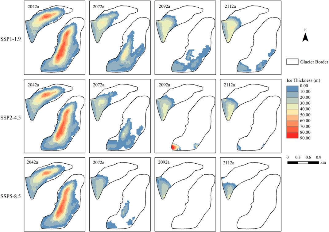
FIGURE 9. Simulated glacier area and thickness results in different years: the 30th year (2042), the 60th year (2072), the 80th year (2092), and the 100th year (2112) in the SSP1-1.9, the SSP2-4.5, and the SSP5-8.5 scenarios.

Though there was no large difference in areas of the glacier in the three climate scenarios before 2025 (Figure 10C), the areas varied a lot in the three climate scenarios after 2040, and the changes were also obvious in the EB and the WB (Figures 10A,B). In the SSP1-1.9 climate scenario, the area of the glacier decreased slowly, while in the other two climate scenarios, the areas decreased fast after 2040 and then decreased slowly from about 2075 and about 2080, respectively. Reducing half of the glacier area, the glacier took about 68, 58, and 48 years, respectively, in the three climate scenarios, which meant the fastest melting was in the SSP5-8.5 climate scenario.

FIGURE 10

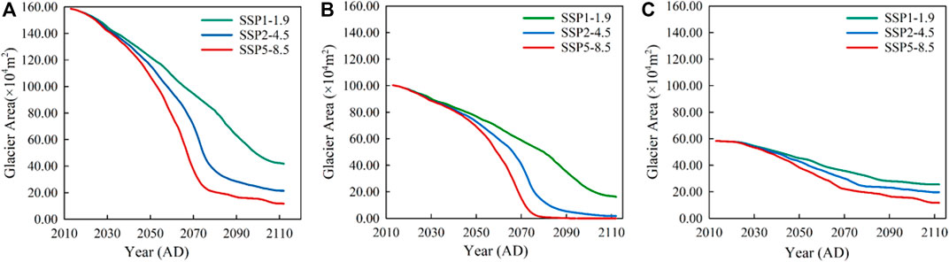
FIGURE 10. Simulated area of the glacier as a function of time in the three climate scenarios: (A) the area of the entire glacier; (B) the area of the EB; and (C) the area of the WB.

More ice melted in the EB compared with that in the WB (Figures 10A,B). As for the EB, the glacier area was about 100 × 10⁴ m² at the beginning and reduced to less than 20 × 10⁴ m² at the end of the simulation period in all the climate scenarios, whereas the maximum of the area loss was less than 50 × 10⁴ m² in the WB, in the SSP5-8.5 climate scenario. The difference between the two branches was derived from the difference in the elevations, and the average elevation of the EB was about 124 m lower than that of the WB.

3.2 The Glacier Ice Volume

In Figure 11C, the volumes of the glacier decreased quickly till 2075 and 2080 in the SSP2-4.5 and the SSP5-8.5 climate scenarios, while the volumes of the glacier remained about 1,000 × 10⁴ m³ after 2100 in the SSP1-1.9 climate scenario. In the SSP5-8.5 climate scenario, after 63 years, the ice volume of the glacier became only 7% of that in 2013, while in the SSP1-1.9 climate scenario, 23% of the ice volume still remained. Thus, from 2013 to 2075, the average loss of the ice volume was −93.1 × 10³ m²·a⁻¹ in the SSP5-8.5 climate scenario (−87.1 × 10⁴ m³·a⁻¹ in the SSP2-4.5 scenario and −76.9 × 10⁴ m³·a⁻¹ in the SSP1-1.9 scenario).

FIGURE 11

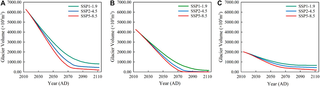
FIGURE 11. Simulated ice volume of the glacier as a function of time in the three climate scenarios: (A) the ice volume of the entire glacier; (B) the ice volume of the EB; and (C) the ice volume of the WB.

The melting in the EB was much more severe than that in the WB (Figures 11A,B). At the beginning of the simulation period, the volume of the EB was twice the volume of the WB, but at the end of the simulation period, the volumes of the EB were nearly zero, while the volumes of the WB still retrained about 200 × 10⁴ m³·a⁻¹ to 650 × 10⁴ m³·a⁻¹ in the three climate scenarios.

3.3 The Glacier Meltwater

In the study, the annual glacier meltwater was the mass loss of the glacier in a year.

The glacier meltwater did not decrease during the whole 100-year period (Figure 12A), because the peak meltwater happened in 2035 and 2038 in the SSP2-4.5 and the SSP5-8.5 climate scenarios, respectively. In the SSP1-1.9 climate scenario, the meltwater decreased and kept about 10 × 10⁴ m³ after 2100; in the SSP2-4.5 climate scenario, the peak meltwater in 2035 was about 131.76 × 10⁴ m³; in the SSP5-8.5 climate scenario, the peak meltwater in 2038 was about 155.89 × 10⁴ m³. Even if, the meltwater decreased without peak value in the SSP1-1.9 climate scenario during the 100 years, the values of meltwater became larger than those in the other two climate scenarios after 2070 for the slower reduction in values of the meltwater. The meltwater was approximately 80 × 10⁴ m³ around 2065 in the three climate scenarios, and the value of meltwater was half of the peak meltwater in the SSP5-8.5 climate scenario, besides, the time—2065, was in the middle of time when the EB did not disappear in the SSP1-1.9 climate scenario.

FIGURE 12

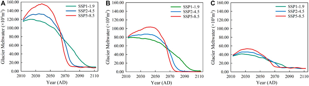
FIGURE 12. Simulated meltwater of the glacier as a function of time in the three climate scenarios: (A) the meltwater of the entire glacier; (B) the meltwater of the EB; and (C) the meltwater of the WB.

The peak meltwater of the EB and the WB occurred in different time (Figures 12B,C). In the SSP1-1.9 climate scenario, there was no peak meltwater in Figure 12B, while the peak meltwater in Figure 12C was in 2025. In the SSP2-4.5 climate scenario, the peak meltwater of the EB was in 2036, and the peak meltwater of the WB was in 2027. In the SSP5-8.5 climate scenario, the peak meltwater of the EB was in 2044, and the peak meltwater of the WB was in 2033.

4 Discussions

4.1 The Glacier Runoff in the Future

Accounting for about 70% of the replenishment to Urumqi River headwaters, the runoff of Urumqi Glacier No. 1 is significant to the Urumqi River. The glacier runoff included the precipitation in the glacier area and the glacier meltwater, which is shown in Figure 13.

FIGURE 13

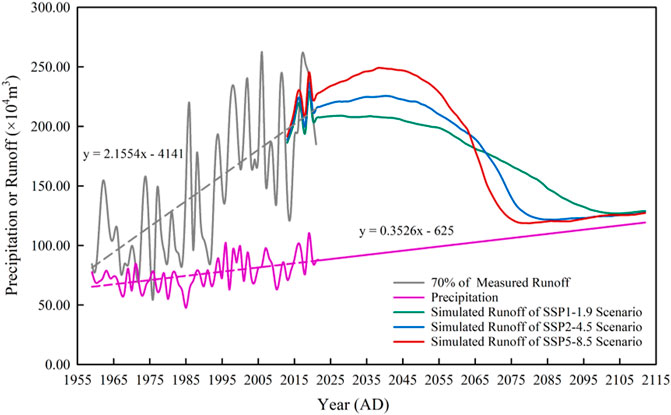
FIGURE 13. Simulated glacier runoff in the three climate scenarios that compared with measured runoff.

70% of the measured runoff from 1959 to 2019 is shown in Figure 13, with an upward trend. Although the precipitation from 1959 to 2019 also showed an increasing trend, the trend line slope of the precipitation was much smaller than that of 70% of the measured runoff, which implicated that the glacier meltwater kept increasing faster than the precipitation from 1959 to 2019. Compared with the sum of annual precipitation and annual simulated glacier meltwater from 2012 to 2019, the 70% of the measured runoff matched the upward trend of the sum. Hence, the simulation results from 2012 to 2019 were consistent with the measured data well.

From 2020 to 2070, the glacier runoff was mainly from the glacier meltwater, and the changes in the runoff were similar to those of the glacier meltwater. In the SSP1-1.9 climate scenario, the runoff decreased gently with no peak runoff. In the SSP2-4.5 climate scenario, the peak runoff occurred in 2040, and the year was 5 years later than the peak-meltwater year (2035). In the SSP5-8.5 climate scenario, the peak runoff was in 2039, this year was only 1 year later than the peak-meltwater year (2038) in this climate scenario.

After 2070, the runoff was mainly influenced by the precipitation except the runoff in the SSP1-1.9 scenario. As the annual glacier meltwater after 2070 in the SSP2-4.5 and SSP5-8.5 scenarios was less than 10 × 10⁴ m³, and the precipitation was more than 80 × 10⁴ m³ from 2070, the runoff would increase with the increment in the precipitation. However, the glacier meltwater decreased to 10 × 10⁴ m³ from 2100 in the SSP1-1.9 scenario, so from 2070 to 2100, the runoff in this climate scenario was mainly from the glacier meltwater.

With the combination of the projected precipitation and the simulated glacier meltwater from 2013, the meltwater percentages of the whole glacier runoff are displayed in Figure 14. It occurred in 2056 (SSP1-1.9), 2060 (SSP2-4.5), and 2062 (SSP5-8.5) when the amount of meltwater was the same as precipitation, and then precipitation played a dominant role. Based on the simulated results, the contribution of glacier meltwater to the total glacier runoff gradually decreased.

FIGURE 14

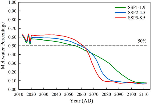
FIGURE 14. The meltwater percentage to the entire glacier runoff. The dashed line denotes that the meltwater accounted for half of the entire glacier runoff.

4.2 The Disappearance of the East Branch

According to the percentages of the EB, the EB nearly disappeared at the end of the simulated period in all the climate scenarios. The area percentages, ice volume percentages, and meltwater percentages of the EB to the whole glacier were not affected by the climate scenario in the first 5 decades. With different ice temperatures set in the climate scenarios under climate change, the percentages of the EB reduced fastest in the SSP5-8.5 climate scenario, and the percentages of the WB gradually increased.

As for the area percentages (Figure 15A), the contribution of the EB hardly changed until 2062 but rapidly decreased after that, especially in the SSP5-8.5 scenario. The area percentages of the EB did not change under all the climate scenarios before 2062, and it was over 60% of the whole glacier areas. After 2062, the area percentages of the EB rapidly decreased until its disappearance, and it was only about 30 years from 60% to zero under the SSP5-8.5 scenario.

FIGURE 15

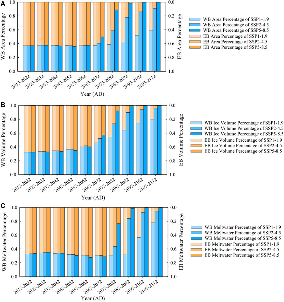
FIGURE 15. The (A) area, (B) ice volume, and (C) meltwater percentage of the EB (WB) to the entire glacier in the three climate scenarios.

With the glacier rapidly retreated, the EB ice volume percentages to the whole glacier of Urumqi Glacier No. 1 continued to decrease (Figure 15B). The ice volume percentages under all the climate scenarios from 2013 to 2052 maintained similar. Subsequently, the EB ice percentages showed the significant differences after 2052. In the SSP5-8.5 scenario, the EB disappeared first and the EB ice volume percentage was zero. However, under the SSP1-1.9 scenario, the EB ice volume percentage was still 35%. It took about only 15 years for the ice volume percentages to decrease from 60% to 20% in the SSP5-8.5 scenario, while it took 25 and 50 years under the climate scenarios of SSP2-4.5 and SSP1-1.9, respectively.

The EB meltwater percentages almost did not change under all the climate scenarios (Figure 15C), remaining at about 70%–65% before 2072. With the glacier rapidly retreating, the WB meltwater gradually became the main part of the total meltwater, and the meltwater percentages were over 90% in 2090 and in 2080 under the climate scenarios of SSP2-4.5 and SSP5-8.5.

With the climate warming, the accumulation area quickly reduced with the increasing ELA. The EB was under full melting from the glacier terminus to the head area when its accumulation area reduced to zero, while the WB still remained a little accumulation area at the end of the 100-year period. Therefore, only the EB almost disappeared at the end of the 100-year period.

Outside the Elmer/Ice three-dimensional model which was used to Urumqi Glacier No. 1, previous one-dimensional and two-dimensional simulation works also projected that the glacier would retreat and disappear in the future and the EB would disappear earlier than the WB (Li, 2010; Duan et al., 2012; Gao et al., 2018). Compared with the previous simulation works, though changes of the EB were similar in different models, the important values of the glacier in the Elmer/Ice three-dimensional model, especially the ice volume and runoff, were much more accurate than the values in the one-dimensional or two-dimensional models.

5 Conclusion

This study used the Elmer/Ice ice-flow model to simulate the evolution of Urumqi Glacier No. 1, which combined the glacier geometry, measured ice-flow velocity, mass balance, and borehole ice temperature, based on the climate scenarios of SSP1-1.9, SSP2-4.5, and SSP5-8.5 in the Sixth Assessment Report of IPCC.

The ice volume of Urumqi Glacier No. 1 will be less than 10% at the end of the ablation, which is all the contribution from the glacier of the WB. Under all the climate scenarios, the ice volume curve recedes linearly before 2080; the glacier area retreats rapidly in the early 100-year period and slowly by the late ablation; the glacier runoff peaks are most likely to occur in 2040 under the climate scenarios of SSP2-4.5 and SSP5-8.5 and then decrease rapidly until they infinitely close to the precipitation curve.

The ice volume and area of the EB decrease more rapidly than that of the WB under the unequivocal warming of the climate system, while the peak runoff time of the WB is much earlier. The ice volume, area, and runoff of the EB contributed more to the entire glacier in the early 100-year period, while WB contributed more by the late ablation.

Urumqi Glacier No. 1 is a typical continental glacier and is also important headwaters of the Urumqi River. The glaciers with similar properties to Urumqi Glacier No. 1 might gradually disappear under all the climate scenarios in IPCC, which is an inevitable trend of glacier evolution under the climate change and impacts the changes in runoff at the headwaters of the river that originated in the mountains and local economy and ecosystems.

Data Availability Statement

The original contributions presented in the study are included in the article/Supplementary Material; further inquiries can be directed to the corresponding author.

Author Contributions

ZW and BY: conceptualization; PJ and SJ: data curation; PJ: formal analysis; PJ, BY, and SA: methodology; ZW: resources; PJ: software; PJ: visualization; PJ: writing original draft.

Funding

Our study was supported by the National Natural Science Foundation of China (41941010).

Conflict of Interest

The authors declare that the research was conducted in the absence of any commercial or financial relationships that could be construed as a potential conflict of interest.

Publisher’s Note

All claims expressed in this article are solely those of the authors and do not necessarily represent those of their affiliated organizations, or those of the publisher, the editors, and the reviewers. Any product that may be evaluated in this article, or claim that may be made by its manufacturer, is not guaranteed or endorsed by the publisher.

Acknowledgments

We thank the reviewers for their constructive comments that helped us to polish this manuscript.

References

Ai, S., Yan, B., Wang, Z., and Lin, G. (2019). Projection of Long-Term Changes of Mountain Glacier Based on GIS Grid Operation Method [J]. Chin. J. Polar Res. 31 (3), 267–275. doi:10.13679/j.jdyj.20180050

CrossRef Full Text | Google Scholar

Bahr, D. B., Pfeffer, W. T., Sassolas, C., and Meier, M. F. (1998). Response Time of Glaciers as a Function of Size and Mass Balance: 1. Theory. J. Geophys. Res. 103 (B5), 9777–9782. doi:10.1029/98jb00507

CrossRef Full Text | Google Scholar

Barry, R. G. (2006). The Status of Research on Glaciers and Global Glacier Recession: A Review. Prog. Phys. Geogr. Earth Environ. 30 (3), 285–306. doi:10.1191/0309133306pp478ra

CrossRef Full Text | Google Scholar

Ding, Y., Liu, S., Li, J., and Shangguan, D. (2006). The Retreat of Glaciers in Response to Recent Climate Warming in Western China[J]. Ann. Glaciol. 43, 97–105.

CrossRef Full Text | Google Scholar

Dong, Z., Qin, D., Ren, J., Li, K., and Li, Z. (2012). Variations in the Equilibrium Line Altitude of Urumqi Glacier No.1, Tianshan Mountains, Over the Past 50 Years. Chin. Sci. Bull. 57 (36), 4776–4783. doi:10.1007/s11434-012-5524-1

CrossRef Full Text | Google Scholar

Duan, K., Yao, T., Wang, N., and Liu, H. (2012). Numerical Simulation of Urumqi Glacier No. 1 in the Eastern Tianshan, Central Asia from 2005 to 2070. Chin. Sci. Bull. 57 (34), 4505–4509. doi:10.1007/s11434-012-5469-4

CrossRef Full Text | Google Scholar

Gao, H., Li, H., Duan, Z., Ren, Z., Meng, X., and Pan, X. (2018). Modelling Glacier Variation and its Impact on Water Resource in the Urumqi Glacier No. 1 in Central Asia. Sci. Total Environ. 644, 1160–1170. doi:10.1016/j.scitotenv.2018.07.004

PubMed Abstract | CrossRef Full Text | Google Scholar

Haeberli, W., Cihlar, J., and Barry, R. G. (2000). Glacier Monitoring within the Global Climate Observing System. Ann. Glaciol. 31, 241–246. doi:10.3189/172756400781820192

CrossRef Full Text | Google Scholar

Immerzeel, W. W., Van Beek, L. P. H., and Bierkens, M. F. P. (2010). Climate Change Will Affect the Asian Water Towers. Science 328 (5984), 1382–1385. doi:10.1126/science.1183188

PubMed Abstract | CrossRef Full Text | Google Scholar

Jia, Y., Li, Z., Jin, S., Xu, C., Zhang, M., and Deng, H. (2019). Changes of the Runoff and its Components in Urumqi Glacier No.1 Catchment, Tianshan Mountains, 1959-2017. J. Glaciol. Geocryol. 41 (6), 1302–1312. doi:10.7522/j.issn.1000-0240.2019.1197

CrossRef Full Text | Google Scholar

Kraaijenbrink, P. D. A., Bierkens, M. F. P., Lutz, A. F., and Immerzeel, W. W. (2017). Impact of a Global Temperature Rise of 1.5 Degrees Celsius on Asia's Glaciers. Nature 549 (7671), 257–260. doi:10.1038/nature23878

PubMed Abstract | CrossRef Full Text | Google Scholar

Li, H. (2010). Glacier Dynamic Models and Their Applicability for the Alpine Glaciers in China [D]. Beijing(China): Chinese Academy of Sciences.

Google Scholar

Li, K., Li, Z., Gao, W., and Wang, L. (2011a). Recent Glacial Retreat and its Effect on Water Resources in Eastern Xinjiang. Chin. Sci. Bull. 56 (33), 3596–3604. doi:10.1007/s11434-011-4720-8

CrossRef Full Text | Google Scholar

Li, X., Li, Z., Wang, W., Wang, P., and Li, S. (2013). Variations on Equilibrium Line Altitude of the Glacier No.1 at the Headwaters of Urumqi River, during 1959-2009. J. Arid Land Resour. Environ. 27 (02), 83–88. doi:10.13448/j.cnki.jalre.2013.02.036

CrossRef Full Text | Google Scholar

Li, Z., Li, K., and Wang, L. (2010). Study on Recent Glacier Changes and Their Impact on Water Resources in Xinjiang, North-Western China. Quat. Sci. 30 (1), 96–106.

Google Scholar

Li, Z., and Wang, F. (2016). Annual Mass Balance of Glacier No.1 at the Source of Urumqi River from 2006 to 2012. Lanzhou, Gansu Province, China: National Cryosphere Desert Data Center. Available at: www.ncdc.ac.cn. doi:10.12072/Tianshan.013.2017.db

CrossRef Full Text | Google Scholar

Li, Z., Li, H., and Chen, Y. (2011b). Mechanisms and Simulation of Accelerated Shrinkage of Continental Glaciers: A Case Study of Urumqi Glacier No. 1 in Eastern Tianshan, Central Asia. J. Earth Sci. 22 (4), 423–430. doi:10.1007/s12583-011-0194-5

CrossRef Full Text | Google Scholar

IPCC (2021). “Summary for Policymakers,” in Climate Change 2021: The Physical Science Basis. Contribution of Working Group I to the Sixth Assessment Report of the Intergovernmental Panel on Climate Change. Editors V. Masson-Delmotte, P. Zhai, A. Pirani, S.L. Connors, C. Péan, S. Bergeret al. (Cambridge, United Kingdom and New York, NY, USA: Cambridge University Press), 3–32. doi:10.1017/9781009157896.001

CrossRef Full Text | Google Scholar

Pörtner, H. O., Roberts, D. C., Masson-Delmotte, V., Zhai, P., Tignor, M., Poloczanska, E., et al. (2019). “The Ocean and Cryosphere in a Changing Climate,” in IPCC Special Report on the Ocean and Cryosphere in a Changing Climate. Cambridge, United Kingdom and New York, NY: Cambridge University Press, 755 pp. doi:10.1017/9781009157964

CrossRef Full Text | Google Scholar

Qin, D., Yao, T., Ding, Y., and Ren, J. (2016). English-Chinese Dictionary of Cryospheric Science (Revised Edition). Beijing, China: China Meteorological Press.

Google Scholar

Ren, Z., Gao, H., Elser, J. J., and Zhao, Q. (2017). Microbial Functional Genes Elucidate Environmental Drivers of Biofilm Metabolism in Glacier-Fed Streams. Sci. Rep. 7 (1), 12668. doi:10.1038/s41598-017-13086-9

PubMed Abstract | CrossRef Full Text | Google Scholar

Sun, B., He, M., Zhang, P., Jiao, K., Wen, J., and Li, Y. (2003). Determination of Ice Thickness, Subice Topography and Ice Volume at Glacier No.1 in the Tien Shan, China, by Ground Penetrating Radar[J]. Chin. J. Polar Res. 15 (01), 35–44.

Google Scholar

Sun, M., Li, Z., Yao, X., and Jin, S. (2013). Rapid Shrinkage and Hydrological Response of a Typical Continental Glacier in the Arid Region of Northwest China - Taking Urumqi Glacier No.1 as an Example. Ecohydrol. 6 (6), 909–916. doi:10.1002/eco.1272

CrossRef Full Text | Google Scholar

Wang, P., Li, Z., Li, H., Wang, W., and Yao, H. (2014). Comparison of Glaciological and Geodetic Mass Balance at Urumqi Glacier No. 1, Tian Shan, Central Asia. Glob. Planet. Change 114, 14–22. doi:10.1016/j.gloplacha.2014.01.001

CrossRef Full Text | Google Scholar

Wang, Z., Lin, G., and Ai, S. (2019). How Long Will an Arctic Mountain Glacier Survive? A Case Study of Austre Lovénbreen, Svalbard. Polar Res. 38, 3519. doi:10.33265/polar.v38.3519

CrossRef Full Text | Google Scholar

Xia, M., Li, Z., and Wang, W. (2012). Research on Characteristics Variation of East and West Branches of Glacier No.1 at the Headwaters of Urumqi River [J]. J. Arid Land Resour. Environ. 26 (9), 40–44. doi:10.13448/j.cnki.jalre.2012.09.034

CrossRef Full Text | Google Scholar

Xu, C., Li, Z., Li, H., Wang, F., and Zhou, P. (2019). Long-Range Terrestrial Laser Scanning Measurements of Annual and Intra-Annual Mass Balances for Urumqi Glacier No. 1, Eastern Tien Shan, China. Cryosphere 13 (9), 2361–2383. doi:10.5194/tc-13-2361-2019

CrossRef Full Text | Google Scholar

Xu, X., Pan, B., Hu, E., Li, Y., and Liang, Y. (2011). Responses of Two Branches of Glacier No.1 to Climate Change from 1993 to 2005, Tianshan, China. Quat. Int. 236 (1-2), 143–150. doi:10.1016/j.quaint.2010.06.013

CrossRef Full Text | Google Scholar

Yang, Z. (1991). Glacier Water Resources in China[M]. Lanzhou: Gansu Science and Technology Press, 74–78.

Google Scholar

Ye, B., Yang, D., Jiao, K., Han, T., Jin, Z., Yang, Z., et al. (2005). The Urumqi River Source Glacier No.1, Tianshan, China: Changes over the Past 45 Years. Geophys. Res. Lett. 32 (21), L21504. doi:10.1029/2005gl024178

CrossRef Full Text | Google Scholar

Yue, X., Li, Z., Wang, F., Li, H., and Shen, S. (2021). The Characteristics of Surface Albedo on the Urumqi Glacier No.1 during the Ablation Season in Eastern Tien Shan[J]. J. Glaciol. Geocryol. 43 (5), 1–12. doi:10.7522/j.issn.1000-0240.2020.0097

CrossRef Full Text | Google Scholar

Zemp, M., Frey, H., Gärtner-Roer, I., Nussbaumer, S. U., Hoelzle, M., Paul, F., et al. (2015). Historically Unprecedented Global Glacier Decline in the Early 21st Century. J. Glaciol. 61 (228), 745–762. doi:10.3189/2015jog15j017

CrossRef Full Text | Google Scholar

Zemp, M., Hoelzle, M., and Haeberli, W. (2009). Six Decades of Glacier Mass-Balance Observations: A Review of the Worldwide Monitoring Network. Ann. Glaciol. 50 (50), 101–111. doi:10.3189/172756409787769591

CrossRef Full Text | Google Scholar

Zhang, L., Tang, X., Yang, S., Xu, S., and Zhang, Y. (2017). Numerical Simulations of East Antarctic Ice Sheet Based on the Elmer/Ice Model. Chin. J. Polar Res. 29 (3), 390–398. doi:10.13679/j.jdyj.2017.3.390

CrossRef Full Text | Google Scholar

Zhao, L., Tian, L., Zwinger, T., Ding, R., Zong, J., Ye, Q., et al. (2014). Numerical Simulations of Gurenhekou Glacier on the Tibetan Plateau. J. Glaciol. 60 (219), 71–82. doi:10.3189/2014jog13j126

CrossRef Full Text | Google Scholar

Zhou, Z., Li, Z., Li, H., and Jing, Z. (2009). The Flow Velocity Features and Dynamic Simulation of the Glacier No.1 at the Headwaters of Urumqi River, Tianshan Mountains[J]. J. Glaciol. Geocryol. 31 (01), 55–61.

Google Scholar