Evaluating the Minimum Number of Earthquakes in Empirical Site Response Assessment: Input for New Requirements for Microzonation in the Swiss Building Codes

Site-specific hazard analyses and microzonation are important products for densely populated areas and facilities of special risk. The empirical amplification function is classically estimated using the standard spectral ratio (SSR) approach. The SSR simply consists in comparing earthquake recordings on soil sites with the recording of the same earthquake on a close-by rock reference. Recording a statistically significant number of earthquakes to apply the SSR can however be difficult, especially in low seismicity areas and noisy urban environments. On the contrary, computing the SSR from too few earthquakes can lead to an uncertain evaluation of the mean amplification function. Defining the minimum number of earthquake recordings in empirical site response assessment is thus important. We compute empirical amplification functions at 60 KiKnet sites in Japan from several hundred earthquakes and three Swiss sites from several tens of earthquakes. We performed statistical analysis on the amplification functions to estimate the geometric mean and standard deviation and more importantly to determine the distribution law of the amplification factors as a function of the number of recordings. Independent to the site and to the frequency, we find that the log-normal distribution is a very good approximation for the site response. Based on that, we develop a strategy to estimate the minimum number of earthquakes from the confidence interval definition. We find that 10 samples are the best compromise between minimizing the number of recordings and having a good statistical significance of the results. As a general rule, a minimum of 10 uncorrelated earthquakes should be considered, but the higher the number of earthquakes, the lower the uncertainty on the geometric mean of the site amplification function. Moreover, the linear site response is observed to be independent to the intensity of the ground motion level for the analyzed dataset.

Introduction

Site effects can significantly increase the seismic hazard and risk locally. Unconsolidated deposits such as thick and soft sediments in sedimentary basins are prone to strongly amplify the ground motion. Site effects are caused, among others, by the seismic impedance between rock and sediments, the 1D, 2D and 3D resonances, and the edge-generated surface waves. In turn, the site response can vary significantly from one site to another (site-to-site variability, e.g., Bindi et al., 2009; Hollender et al., 2015; Bindi et al., 2017; Imtiaz et al., 2018; Perron et al., 2018) and from one earthquake to another (within-site variability, e.g., Thompson et al., 2012; Ktenidou et al., 2016; Ktenidou et al., 2017; Maufroy et al., 2017; Perron, 2017; Zhu et al., 2018; Zhu et al., 2022). At large ground motion levels, non-linear effects in specific soils will increase the site response uncertainty as well (Régnier et al., 2013; Régnier et al., 2016). Understanding and reducing the ground motion estimation uncertainty is important for Probabilistic Seismic Hazard Assessment, especially at a long return period (Bommer and Abrahamson, 2006). The site-to-site and within-site variabilities have practical implications for site-specific study and microzonation, for instance on the spatial resolution and required duration of the instrumentation.

The within-site variability is very small when estimated from 1D SH site response analysis because it is a strong simplification of the real phenomena. On the contrary, approaches based on direct observations from real earthquake recordings are appropriate for analyzing the variability of the site response. One of the most commonly used approaches to measure the empirical amplification function is the standard spectral ratio (SSR) introduced by Borcherdt (1970). It consists in performing the ratio in the Fourier domain between the signal recorded at one station on sediments and the signal obtained at another station located nearby on a stiffer site condition (i.e., a rock site) for the same earthquake. However, in noisy urban areas in regions of low-to-moderate seismicity, recording earthquakes with a good signal-to-noise ratio (SNR) can require several months, if not years. It is thus important to estimate the number of earthquakes that should be recorded at the sites to evaluate the empirical site amplification function based on the desired accuracy.

The main goal of this work is to define, for the specification in the Swiss building SIA 261/1 (SIA, 2020), the minimum number of earthquakes in empirical site effect assessment. We first evaluate the stability and validity of the mean amplification as a function of the number of earthquake recordings used to compute it. The variations of the mean amplification are expected to be directly related to the within-site variability at each site. To verify that, we estimate the SSR and surface-to-borehole spectral ratio (SBSR) amplification function for stations of the Swiss strong motion network and of the Japanese KiKnet network having recorded hundreds of earthquakes. We use this large amount of data to determine the statistical distribution of the site amplification. Based on the statistical distribution, we propose an analytic equation predicting the variation of the mean amplification according to the standard deviation and to the number of recorded events. We also determined the dependence on the mean amplification functions of the ground motion intensity, measured as the peak ground acceleration (PGA).

Method and Resources

In Switzerland, we developed a waveform database covering the time period from January 1998 to September 2019. Waveforms at each Swiss site were selected according to a magnitude–distance filter. In Japan, the database is covering the time period from October 1997 to March 2016. The SSR is computed for each component individually or the mean of the two horizontal components and can be noted as follows:

$SS{R}_i\left(f\right)=\frac{FA{S}_{Si}\left(f\right)}{FA{S}_{Ri}\left(f\right)},(1)$

where $SS{R}_i\left(f\right)$ is the SSR for the $ith$ component as a function of frequency $f$ and $FA{S}_{Si}$ and $FA{S}_{Ri}$ are respectively the Fourier amplitude spectra (FAS) at the site and at the reference computed over the $ith$ component. The SSR approach is based on the assumption that the earthquake source and wave propagation along the path are the same between the site and the reference and thus canceled out when performing the spectral ratio between the two. This assumption is valid if the site-to-reference distance (R_STA) is much smaller than the hypocentral distance (Rh). In practice, adopting Rh > 10R_STA is considered to be enough, even though a certain part of the SSR variability can probably be explained by a remaining influence of the source and of the path (Borcherdt, 1970; Perron, 2017). The ground motion amplification at the reference station is assumed to be negligible, that is to say, equal to one at every frequency. In practice, it is never the case (Hollender et al., 2017; Hollender et al., 2018; Hobiger et al., 2021), so the SSR-based amplification factors are not absolute but are always relative to the considered reference. One of the main limitations of the SSR is of having a rock outcropping susceptible to be used for the reference site located not too far from the considered site of interest. An alternative to the classical SSR is to deploy one station at the earth’s surface on sediments and the second at the same location but in a borehole deep enough to reach the geophysical bedrock. This so-called SBSR approach has the advantage of solving the between-station distance limitation but introduces some new difficulties because of the seismic wave reflection at the earth’s surface. The upgoing and downgoing waves are indeed fully constructive at the earth’s surface, although they can be destructive at certain frequencies at depth (Cadet et al., 2012). However, in the context of analyzing only the variability of the site response, the downgoing wave interaction can reasonably be neglected (Cadet et al., 2012; Hollender et al., 2018). We followed the same procedure for every computation of the site response in Switzerland and Japan. This procedure is as follows:

1) Automatic quality checks of earthquake recordings and automatic picking of the P and S wave arrival (T_P, T_S) through a time–frequency analysis;

2) Selection of earthquakes with hypocentral distance at least five times the interstation distance (R_STA);

3) Selection of the signal window between T_P and the coda defined by 3.3T_S–2.3T_P (Perron et al., 2017) and of the noise window before T_P and of the same duration as the signal window. Site and reference use the same time windows;

4) Computation of the FAS for the noise and the signal window;

5) Computation of the horizontal mean FAS using the quadratic mean: $\sqrt{\frac{N^2+E^2}{2}}$;

6) Smoothing and resampling of the horizontal mean FAS on a logarithmic scale using the Konno and Ohmachi (1998) approach with a b-value of 50;

7) Estimation of the SNR;

8) Selection of earthquakes with SNR > 5 over at least a two-octave frequency band window both at the site and at the reference;

9) Spectral ratio computation between the horizontal mean FAS at the site and at the reference for each earthquake;

10) Estimation of the within-site events geometric mean and standard deviation at each frequency;

11) Detection of outliers as a group of samples of probability <0.1% over a frequency band larger than one octave;

12) Outliers are discarded, and the geometric mean and standard deviation are recomputed

Figure 1 shows an example of the SBSR computation in Japan.

FIGURE 1

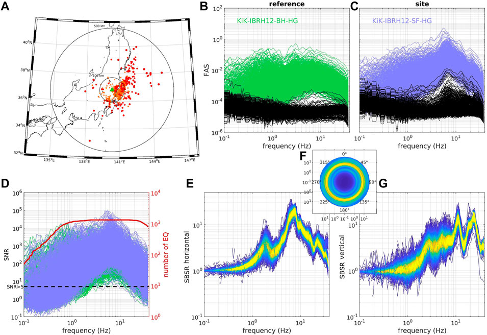
FIGURE 1. Example of the surface-to-borehole spectral ratio (SBSR) computation at KiKnet station IBRH12 in Japan. (A) The map shows the location of the site (green triangle) and the epicenters of the selected earthquakes (yellow-to-red dot according to the earthquake magnitude). Panels (B) and (C) present the power spectral density (PSD) for the noise (black lines) and for the earthquake recording on the horizontal mean component at the site (blue lines) and at the reference (green lines). Panel (D) indicates the SNR at the site (blue lines) and at the reference (green lines), as well as the number of earthquakes spectrum with SNR > 5 (red line) as a function of frequency. The distribution of the SBSR as a function of frequency for the horizontal mean component (E), for the horizontal as a function of the azimuth (F), and for the vertical (G) component. The color scale indicates the density of lines, each line corresponding to the SBSR of one single earthquake.

Standard Spectral Ratio and Surface-to-Borehole Spectral Ratio Results

In total, SSR is estimated from three pairs of stations where approximately 100 good-quality earthquakes have been recorded in Switzerland, and SBSR is computed from 60 pairs of surface-to-borehole stations with up to 2000 good-quality earthquakes in Japan. Figure 2 and Figure 3 respectively show the distribution of the SBSR for 60 pairs of surface-to-borehole stations in Japan and the SSR for the three pairs of surface stations in Switzerland. Figure 4 provides a summary of the number of good-quality earthquake recordings, geometric mean, and geometric standard deviation as a function of frequency in Japan (gray curves) and Switzerland (red curves).

FIGURE 2

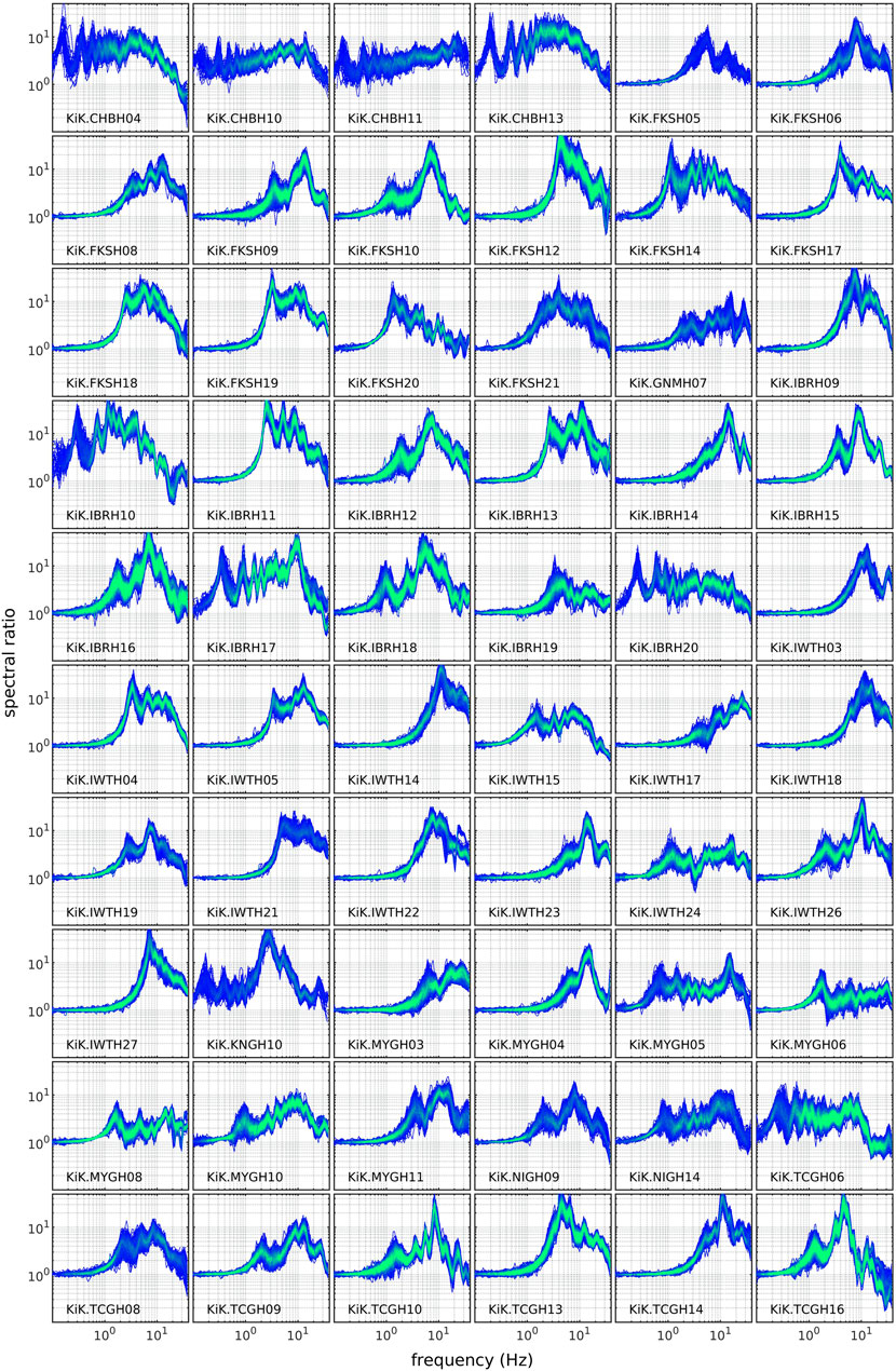
FIGURE 2. Amplification function computed from the SBSR between 60 pairs of stations in Japan. The color from dark blue to light green indicates an increasing density of curves, each curve corresponding to one single earthquake.

FIGURE 3

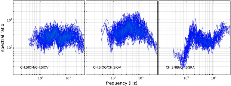
FIGURE 3. Amplification function computed from the standard spectral ratio between 3 pairs of stations in Switzerland. The color from dark blue to light blue indicates an increasing density of curves, each curve corresponding to one single earthquake.

FIGURE 4

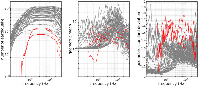
FIGURE 4. Number of good-quality earthquakes (left panel), within-site geometric mean (central panel), and within-site geometric standard deviation (right panel) as a function of frequency for 60 surface-to-borehole spectral ratios in Japan (gray curves) and three standard spectral ratio in Switzerland (red curves).

Figure 2, Figure 3, and Figure 4 clearly show that the amplification functions are different from one site to another, both in terms of mean and standard deviation. It reflects the differences in the geological conditions of the sites, which determine, among others, the fundamental resonance frequency of the site (f₀), here corresponding to the first peak on the amplification function. The within-site standard deviation can also vary drastically from one site to another and depending on the frequency. In Japan, we can separate the amplification functions into two groups: the first group with f₀ > 0.5 Hz, with an amplification function equal to one and low standard deviation (close to 1.05) for frequency below f₀; a second group with f₀ below the minimum frequency of the analysis here (0.1 Hz), and having significant amplification (above one) and high variability at low frequency. It is also clear that the variability of the site response is on average higher in Switzerland than that in Japan. For the Swiss sites, this is probably because of the SSR method imposing relatively high site-to-reference distances and non-negligible site effects at the surface reference station. In Japan, we can observe some anomalies (eye shapes departing from the log-normal distribution) in the amplification function at high frequency (e.g., for stations: KiK-IBRH13; KiK-IBRH17; KiK-TCGH16). It is not possible to clearly determine its origin, but from our experience, this is very probably an artificial artifact because of coupling issues of the borehole instrumentation or because of a modification on the instrumentation at some point due to maintenance of the station for instance.

Distribution of the Within-Site Variability

As we have seen in the previous section, both the mean and standard deviation of the amplification function as a function of frequency are dependent to the geological characteristics of the site itself. However, the nature of the site response distribution is the same independently to the site or to the frequency and has been shown to be well modeled by a log-normal distribution (Ktenidou et al., 2011). In other words, the distribution of the logarithm of the relative amplification of the ground motion between two sites is Gaussian. To qualitatively verify the log-normal distribution of the site response at every frequency, the quantile–quantile (Q–Q) plot and the histogram are represented at frequencies 0.5, 1.0, 2.5, 5.1, 9.9, and 20.6 Hz in Figure 5. The shape of the histograms of the logarithm of the amplification factors represents a Gaussian and Q–Q curves of every site at every frequency are well aligned along the 1/1 line, in particular in the interval $\pm 2\sigma$ to the mean. These indicate that the site response is very well approximated by log-normal distribution at least up to $\pm 2\sigma$. Beyond $2\sigma$, the few non-natural outliers and the limited number of samples increase the scatter of the Q–Q curves, meaning that the log-normal distribution is still valid but interpretations made out of it are less reliable.

FIGURE 5

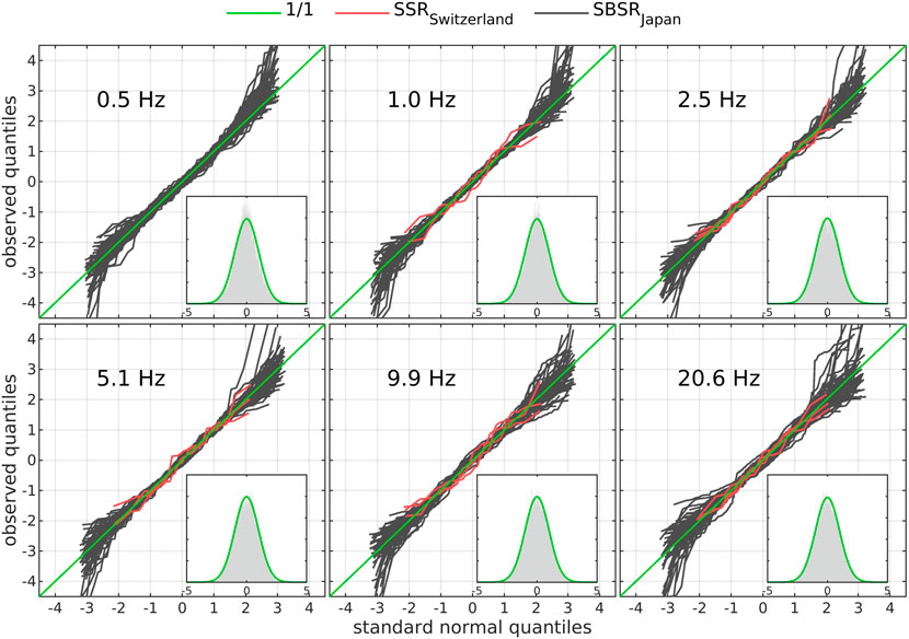
FIGURE 5. Quantile–quantile plot of the logarithm of the amplification factors for 60 surface-to-borehole spectral ratios in Japan (gray curves) and three standard spectral ratios in Switzerland (red curves) at six different frequencies (one panel per frequency). On each panel, the histogram (gray area) of the standard normal distribution computed from the logarithm of the amplification factors at all sites at the corresponding frequency is compared with the best normal distribution fit (green curve).

Proving the log-normal distribution of the amplification function is important because then peculiar statistical properties apply. For example, if a variable $x$ is normally distributed then the distribution of sample means ($\overline{x_n}$) computed from subsets of $n$ samples also are normally distributed. One major output of that is the confidence interval ($Ic$). Given that a sample mean ($\overline{x_n}$) and unbiased standard deviation ($s_n$) have been estimated from a finite number of samples ($n$), the confidence interval is the interval inside which the population mean ($\mu$) for an infinite number of samples has a certain confidence level to be included in. It is defined as follows:

$I{c}_{1-\alpha \%}=\left[\overline{x_n}-Z_{\alpha /2}\frac{s_n}{\sqrt{n}}; \overline{x_n}+Z_{\alpha /2}\frac{s_n}{\sqrt{n}}\right],(2)$

where $Z_{\alpha /2}$ is the critical value that defines the confidence level ($1-\alpha$). For a normal distribution and a confidence level of 95%, $Z_{0.025}$ is equal to 1.96. However, because the number of samples can be sometimes very limited (i.e., only a few earthquakes have been recorded), it is preferable to use the Student distribution, also called t-distribution. This distribution correctly accounts for a small number of samples and tends to be a normal distribution as the number of samples increases. For a Student distribution, the formulation of $I{c}_{1-\alpha \%}$ is the same (Eq. 2), but the estimation of $Z_{\alpha /2}$ is different, as it now also depends on $n$. The evolution of $Z_{\alpha /2,n}$ as a function of $n$ and for the confidence levels 68, 95, 99, and 99.9% is given in Figure 6, left panel. In the following, we will keep using the notation $\overline{x_n}$ and $s_n$ for the measured sample geometric mean and standard deviation, whereas $\mu$ and $\sigma$ represent the population geometric mean and standard deviation of the distribution. For an infinite number of samples, the two notations become equivalent: $\overline{x_{\infty }}=\mu$ and $s_{\infty }=\sigma$. Moreover, we will only focus on the confidence level of 95%, because the 95% confidence interval corresponds approximately to the interval comprised between $\left[-1.96\sigma 1.96\sigma \right]$, which in turn corresponds to the portion where the Q–Q plot best fit the 1/1 line (Figure 5). As the distribution is not normal but log-normal, we accordingly modified the confidence interval formulation. The 95% confidence interval for a log-Student distribution is finally:

$I{c}_{95\%}=\left[\overline{x_n}\ast \frac{1}{\exp \left(Z_{0.025, n}\frac{ln\left(s_n\right)}{\sqrt{n}}\right)};\overline{x_n}\ast \exp \left(Z_{0.025, n}\frac{ln\left(s_n\right)}{\sqrt{n}}\right)\right],(3)$

with $\overline{x_n}$ and $s_n$ respectively the sample geometric mean and standard deviation computed as

$\overline{x_n}=\exp \left(\frac{1}{n}{\displaystyle \sum }_{i=1}^n\ln \left(x_i\right)\right),(4)$

$s_n=\exp \left(\sqrt{\frac{1}{\left(n-1\right)}{\displaystyle \sum _{i=1}^n{\left(\ln \left(x_i\right)-\ln \left({\overline{x}}_n\right)\right)}^2}}\right),(5)$

FIGURE 6

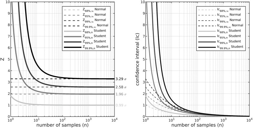
FIGURE 6. Critical value Z (left panel) and confidence interval (right panel) as a function of the number of samples for the confidence levels 68%, 95%, 99%, and 99.9% for the standard normal distribution (dashed lines), and the standard Student distribution (solid lines).

Figure 6 (right panel) shows the evolution of $I{c}_{68\%}$, $I{c}_{95\%}$, $I{c}_{99\%}$, and $I{c}_{99.9\%}$ for a standard normal and standard Student distribution ($\mu =0; \sigma =1$). It illustrates the very rapid reduction of the confidence interval as the number of samples increases, from more than 10 $\sigma$ when $n<10$ to less than 1 $\sigma$ when $n>10$.

Validity of the Confidence Interval Predictions

After demonstrating the validity of the log-normal assumption, we verified the validity of the prediction of $I{c}_{95\%}$ for a Student distribution as a function of the number of earthquakes $n$ by comparing $I{c}_{95\%}$ with the observations in Switzerland and Japan. First, we defined two different confidence intervals:

$I{c}_{95N}\left(n\right)=\left[\overline{x_N}\ast \frac{1}{\exp \left(Z_{0.025, N}\frac{ln\left(s_N\right)}{\sqrt{n}}\right)};\overline{x_N}\ast \exp \left(Z_{0.025, N}\frac{ln\left(s_N\right)}{\sqrt{n}}\right)\right](6)$

$I{c}_{95n}\left(n\right)=\left[\overline{x_n}\ast \frac{1}{\exp \left(Z_{0.025, n}\frac{ln\left(s_n\right)}{\sqrt{n}}\right)};\overline{x_n}\ast \exp \left(Z_{0.025, n}\frac{ln\left(s_n\right)}{\sqrt{n}}\right)\right](7)$

where $\overline{x_N}$ and $s_N$ are respectively the total geometric mean and standard deviation computed over the entire dataset of $\text{N}$ events. $\overline{x_n}$ and $s_n$ are respectively the local geometric mean and standard deviation computed over a subset of $n$ randomly selected events. $I{c}_{95N}\left(n\right)$ is the total 95% confidence interval used to predict the variation of any local mean $\overline{x_n}$ computed from $n$ events. $I{c}_{95n}\left(n\right)$ is the local 95% confidence interval used to predict the interval of variation of the total mean $\overline{x_N}$. This assumes that $\overline{x_N}=\mu$ and $s_N=\sigma$, which is reasonably correct here since N is most of the time much higher than 100 earthquakes.

To estimate the reliability of the confidence interval more quantitatively, we bootstrapped the amplification factors at each frequency over $1000$ random selections of $n$ events, with $n=[2 3 4 6 8 10 14 18 24 32]$. We evaluated the proportion of local means included inside the total confidence interval ($P_1= \overline{x_n}\subset I{c}_{95N}\left(n\right)$), and the proportion of total means included inside the local confidence interval ($P_2= \overline{x_N}\subset I{c}_{95n}\left(n\right)$). Following Eq. 3, $P_1$ and $P_2$ can be written:

$P_1\left(f,n\right)=\frac{1}{1000}{\displaystyle \sum }_{k=1}^{1000}\left(\overline{x_N}\left(f\right)\ast \frac{1}{\exp \left(Z_{0.025, N}\frac{\ln \left(s_N\left(f\right)\right)}{\sqrt{n}}\right)}\le {\overline{x_n}}_k\left(f\right)\le \overline{x_N}\left(f\right)\ast \exp \left(Z_{0.025,N}\frac{\ln \left(s_N\left(f\right)\right)}{\sqrt{n}}\right)\right)(8)$

$P_2\left(f,n\right)=\frac{1}{1000}{\displaystyle \sum }_{k=1}^{1000}\left({\overline{x_n}}_k\left(f\right)\ast \frac{1}{\exp \left(Z_{0.025,n}\frac{\ln \left(s_{nk}\left(f\right)\right)}{\sqrt{n}}\right)} \le \overline{x_N}\left(f\right) \le {\overline{x_n}}_k\left(f\right)\ast \exp \left(Z_{0.025,n}\frac{\ln \left(s_{nk}\left(f\right)\right)}{\sqrt{n}}\right)\right)(9)$

with the inequation equal to 1 when it is true and 0 otherwise. ${\overline{x_n}}_k$ and $s_{nk}$ are respectively the $k^{th}$ local geometric mean and standard deviation computed over a subset of $n$ randomly selected events. If the distribution is perfectly normal, then both $P_1$ and $P_2$ are equal to 95%. However, we do not expect the site response distribution to be perfectly normal at every site and for all frequencies, so a certain convergence to 95% should be observed as the number of events $n$ increases.

Figure 7 shows the bootstrap estimation of $P_1$ and $P_2$ from the amplification function of SIOO/SIOV in Switzerland. First, it is clear that the variability between the 1000 ${\overline{x_n}}_k$ decreases (blue points) as $n$ increases (from top-left to bottom-right panel). This decay seems well predicted by $I{c}_{95N}$ (orange lines). This observation is also supported by $P_1$ which is relatively close to the value of 95% at all frequency and for any $n>2$. For $n=2$ we can observe that $P_1$ is slightly higher than 95% between 10 and 20 Hz. In contrast, $P_2$ shows some significant low values for any $n<10$. However, $P_2$ shows a better agreement with the 95% value as $n$ increases. This observation confirms the good approximation of using the log-normal distribution to model the site amplification variability. $I{c}_{95\%}$ makes a relatively good prediction of the observed variability of $\overline{x_n}$, even when the number of samples is low.

FIGURE 7

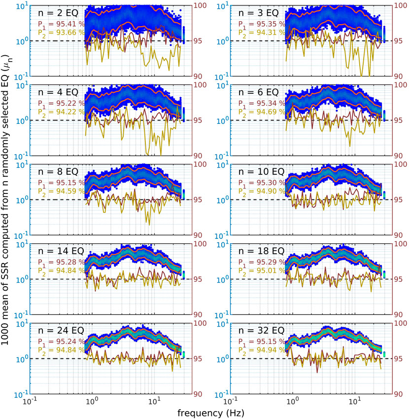
FIGURE 7. Evaluation of P1 (dark brown line) and P2 (light brown line) on the standard spectral ratio computed at Swiss station SIOO/SIOV from 1000 randomly selected subsets of $\mathit{n}=\left[2 3 4 6 8 10 14 18 24 32\right]$ earthquakes (top-left to bottom-right panel). On each panel, the left axis provides the amplification scale and the right axis indicates P1 and P2 proportion in percentages. The 1000 local means $\overline{{\mathit{x}}_{\mathit{n}}}$ are represented according to their density of points from dark blue to light green. The total 95% confidence interval prediction for $\mathit{n}$ events ($\mathit{I}{\mathit{c}}_{95\mathit{N}}$) is represented with orange lines. P1 can be easily visualized by looking at the proportion of $\overline{{\mathit{x}}_{\mathit{n}}}$ points exceeding the $\mathit{I}{\mathit{c}}_{95\mathit{N}}$ (blue points outside the orange lines). There is no way to simply represent P2 here. The number of events, and the mean P1 and P2 over the frequency range are written on each panel.

Now, we follow the same procedure for every three SSR in Switzerland and SBSR in Japan. The corresponding results are given in Figure 8. We can make a similar observation as in Figure 7, $P_1$ is the average equal to the 95% value at all frequency and for every number of events. For the Swiss SSR, we can, however, observe a stronger scatter when the numbers of events are minimum ($n<4$). Again, we observe a stronger deviation of 95% in $P_2$ both in Switzerland and in Japan. In Switzerland, the discrepancy of $P_2$ is higher, especially close to 1 Hz and for $n<6$. $P_2$ is an average lower than 95% but tends to it as $n$ increases. A good agreement is found for $n>6$ and a complete stabilization is observed above 14 events. In Japan, we observed a different behavior, with $P_2$ being too low when $n=2$, and then too high when $2<n<8$ mainly at low frequency (f < 2 Hz). For $n>8$, we observed a good stabilization of $P_2$ with mean values slightly below 95%.

FIGURE 8

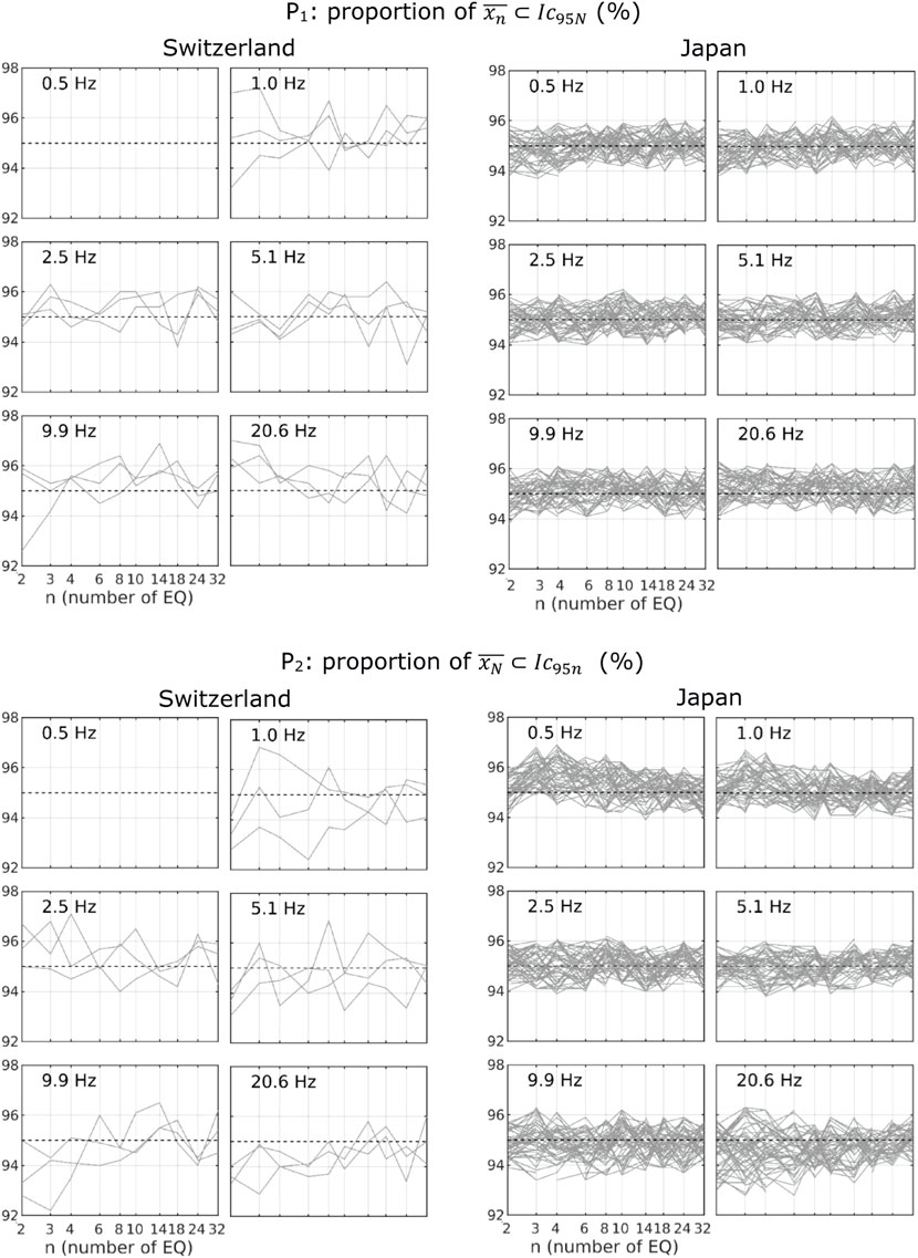
FIGURE 8. Evaluation of P1 and P2 as a function of the number of events $\mathit{n}$ at 6 frequencies (0.5, 1.0, 2.5, 5.1, 9.9, and 20.6 Hz) for three Swiss sites and 60 Japanese sites.

The confidence interval computed from a large site response dataset is a good estimator of what is going to be the behavior of the mean computed from much smaller subsets of even only three earthquakes and for any frequency. However, it is clear that using 10 recordings of earthquakes or above greatly improves the quality of the prediction and the significance of the results. In conclusion, at least 10 events should be considered to have a good statistical significance and to make good use of the confidence interval predicting power.

Variability of the Mean Amplification Function as a Function of the Number of Events

Some questions which arise when evaluating the amplification function at a specific site are as follows: Is the number of earthquake recordings sufficient to accurately estimate the amplification function? Which minimal number of earthquakes ($n_{min}$) should be used to evaluate the site response? Based on the confidence interval definition (Eq. 3), it is clear that the variability of $\overline{x_n}$ depends both on $s_n$ and $n$. Because $s_n$ is site- and frequency-dependent (Figure 4), $n_{min}$ is by consequence also site- and frequency-dependent. In other words, there is no unique value of $n_{min}$ which can be considered for every site response analysis in the world. On the other hand, the property of the site response to be log-normally distributed can be supposed as universal. It is then possible to determine $n_{min}$ for any site response analysis, based on the log-normal distribution assumption and the use of the confidence interval definition.

Provided that the geometric mean $\overline{x_n}$ and standard deviation $s_n$ of the site response has been measured at a particular site over a certain number of earthquakes $n$, it is possible to determine in which confidence interval the population mean for an infinite number of events $\mu$ has a certain confidence level (here 95%) to be included in. It is also possible to predict what will be the reduction of this interval if the number of earthquake observations increases. In the same way, it is possible to determine the number of earthquakes required to limit to a certain level the width of the interval where $\mu$ has a 95% probability to be found within. The width of the interval is independent to the $\overline{x_n}$ and can be defined from Eq. 3 by

$C_{95\%}=\exp \left(Z_{0.025, n}\frac{ln\left(s_n\right)}{\sqrt{n}}\right),(10)$

$C_{95\%}$ is the coefficient of variation between $\mu$ and $\overline{x_n}$ such as $\frac{\overline{x_n}}{C_{95\%}}\le \mu \le C_{95\%}\overline{x_n}$ with a 95% probability. It is now possible to estimate the minimum number of earthquakes required to limit the variation between $\mu$ and $\overline{x_n}$ below a certain coefficient $C_{95\%}$ as

$n_{min}={\left(Z_{0.025, n}\frac{ln\left(s_n\right)}{ln\left(C_{95\%}\right)}\right)}^2(11)$

For example, if the amplification at 1 Hz has been measured from $n=10$ earthquakes with a geometric standard deviation of $s_{10}=1.5$, we can estimate the minimum number of earthquake $n_{min}$ to have $C_{95\%}=1.2$ (20% of variation) with a probability of 95% as

$n_{min}={\left(Z_{0.025,10}\frac{ln\left(s_{10}\right)}{ln\left(C_{95\%}\right)}\right)}^2={\left(2.26\frac{ln\left(1.50\right)}{ln\left(1.20\right)}\right)}^2=25.31\to 26earthquakes$

It is important to note that for a Student distribution, $Z_{0.025, n}$ is the function of $n$. $Z_{0.025, n}$ will decrease very rapidly as the number of measured earthquakes increases (Figure 6). Using Eq. 11 and measured $s_n$ (Figure 4), $n_{min}$ is computed for every site in Switzerland and Japan, and at every frequency. The results are reported in Figure 9. As already discussed, $n_{min}$ is dependent on $s_n$, so it is variable for the different sites and frequency. Swiss SSRs have the highest uncertainty and logically required the highest number of earthquakes for a given coefficient of variation $C_{95\%}$. Table 1 summarizes the minimum number of earthquakes which is valid for 99, 95, and 84% of our sites and frequencies as a function of $C_{95\%}$. For 10 earthquakes recorded, the estimation of the mean is only 40% accurate approximately (${\text{C}}_{95\text{\%}}=1.4$). It is possible to reduce this uncertainty to 25% by recording 20 events (${\text{C}}_{95\text{\%}}=1.25$). Depending on the desired limit for the coefficient of variation of the mean, one can make own estimations of the minimum number of earthquakes using Eq. 7.

FIGURE 9

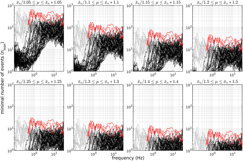
FIGURE 9. Minimum number of earthquakes as a function of frequency for the coefficient of variation ${\mathit{C}}_{95\%}$ equal to 1.05, 1.10, 1.15, 1.20, 1.25, 1.30, 1.4, and 1.5 (panels). KiKnet stations with f₀ > 0.5 Hz are represented in black, KiKnet stations with f₀ < 0.1 Hz are represented in gray, and Swiss stations are represented in red.

TABLE 1

TABLE 1. Minimum number of earthquakes ${\mathit{n}}_{\mathit{min}}$ as a function of the coefficient of variation ${\mathbf{C}}_{95\%}$.

It has to be highlighted that $s_n$ is the key parameter for the estimation of $n_{\mathit{min}}.$ If $s_n$ is wrongly determined, so will be $n_{min}$. One difficulty to have a representative determination of $s_n$ is how to deal with the outliers. Including erratic outliers will artificially increase $s_n$, while removing natural outliers from rare events will truncate the true distribution and reduce $s_n$. Another difficulty is that looking only at the value of $n_{min}$ might not be enough for all sites. One could claim that because the site response has been measured from 30 earthquakes, the statistical significance of the result is good and the coefficient of variation of the mean is low. However, if all the events present the same characteristic and location because they belong to the same cluster of events, then the significance of the results is not good and the true variability of the site response might be strongly underestimated. For instance, Perron (2017) showed that approximately 50% of the within-site variability in 2D and 3D basins comes from the lighting effect, which strongly depends on the source location. This implies that both the number of events and their spatial distribution around the site should be considered in site response analysis.

Dependence of the Site Response Variability on the Intensity of the Ground Motion

The dependence of the site response on the intensity of the ground motion is a complex research topic that interests the community for several decades (e.g., Sánchez-sesma, 1987; Aki, 1993). The non-linear behavior of unconsolidated soil to strong ground motion solicitations is of major interest in engineering seismology. Non-linearity tends to reduce the fundamental resonance frequency of the site, leading to an increase of the hazard at low frequency and a decrease at high frequency (Régnier et al., 2016). In extreme cases, it can also lead to liquefaction phenomena.

One question often arises when speaking about empirical site effects assessment which is: is the measured amplification function from weak ground motion representative of site response to strong ground motion? To address this question, we compute the equivalent of the standard normal distribution ($\mu =0,\sigma =1$) for every individual amplification function at all sites in Switzerland and Japan as

$Zi=\frac{ln\left(xi\right)-ln\left(\overline{x_n}\right)}{ln\left(s_n\right)},(12)$

This common standard normal distribution formulation allows using the site response of every site together. $Zi\left(f\right)$ represent the ith normalized amplification function normally distributed with $\overline{x_n}=0$ and $s_n=1$. Together, it represents about 28,000 normalized amplification functions obtained from thousands of earthquakes recorded at 63 pairs of stations (three Swiss sites and 60 Japanese sites). For each normalized amplification function, we computed on the corresponding waveforms the horizontal mean PGA.

Figure 10 shows the number of events per frequency, the distribution of the PGA and the normalized amplification function for four PGA bins [(0.001 0.01), (0.01 0.1), (0.1 1), and (1 10) m/s²]. First, it should be mentioned that the number of events varies strongly from one PGA bin to another. This explains the apparent differences when looking at the normalized amplification function (black curves) of the different bin. We observe that the normalized amplification function for every PGA bin can be explained by the standard normal distribution, which indicates that no non-linear behavior is observed here. The mean is fairly equal to 0 and the standard deviation is equal to 1 for every frequency of every bin. That demonstrates, first, that the linear behavior characterizes the vast majority of the sites, and second, that the linear site response is independent to the ground motion intensity. Therefore, if we consider a specific site having a linear behavior, the amplification function observed from the weak motion of a small magnitude earthquake will be the same as the one for the strong motion of a large magnitude earthquake, all other things being the same. This highlights the importance and the validity of using the recording of low-to-moderate earthquakes to assess the anelastic amplification functions for larger earthquakes as long as there is no significant non-linear site response at the site of interest.

FIGURE 10

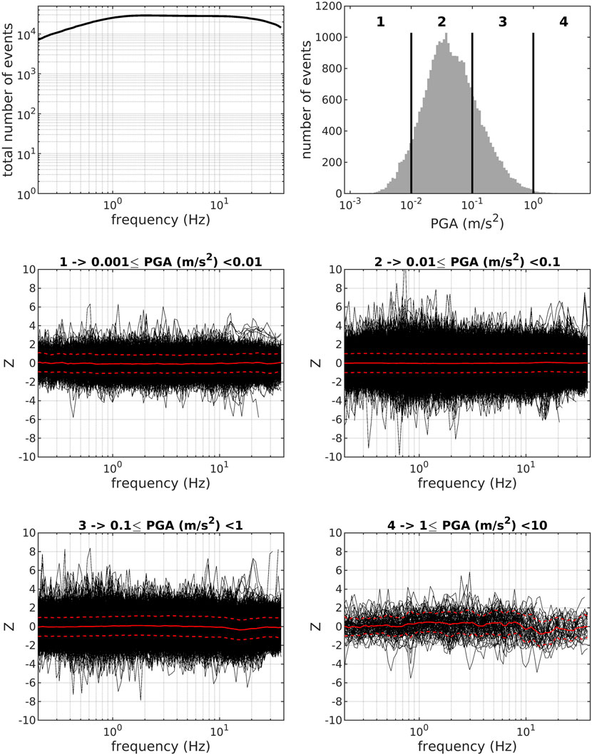
FIGURE 10. Top-left panel: Total number of normalized amplification functions obtain from 3 Swiss SSR distribution and 60 SBSR Japanese distribution and as a function of frequency. Top right: Histogram of the peak ground acceleration (PGA) distribution. From middle left to bottom-right panel: normalized amplification function for four PGA bins and as a function of frequency. The mean and mean plus/minus standard deviation are represented with solid red lines and dotted red lines respectively.

Conclusion

Site effect is a major contributor to the seismic hazard, and its evaluation at specific sites of interest generally requires the recording of several earthquakes. We address here the question of the site response variability and of the minimum necessary number of earthquakes to be recorded.

To address this question, we carefully compute empirical amplification functions at 60 KiKnet sites from several hundred earthquakes and three Swiss sites from several tens of earthquakes. We performed statistical analysis on the amplification function to estimate the geometric mean and standard deviation, and more importantly to determine the distribution law of the amplification factor at each frequency. Independent to the site and to the frequency, we found that the log-normal distribution is a very good approximation for the site response. Based on that we developed a strategy to estimate the minimum number of earthquakes from the confidence interval definition. We first demonstrate the validity of the use of the confidence interval to model the uncertainty of the geometric mean estimation. We found that between 8 and 14 earthquakes are necessary to have a good prediction by the confidence interval, that is to say, a good statistical significance. For most of the sites, 10 samples seem to be the best compromise between minimizing the number of recordings and having a good statistical significance of the results. Based on the confidence interval, we provide the analytic formula to estimate the minimum number of earthquakes to be recorded, as a function of the within-site standard deviation (Eq. 11). We used it on the Swiss and Japanese amplification function and determine, among others, that with a 95% probability: the mean varies by less than 40% for 10 earthquakes, and less than 25% for 20 events.

It is very important to point out that satisfying the minimal number of earthquakes by itself is not sufficient. The selected earthquakes should be uncorrelated and as much evenly distributed around the site as possible to cover the entire variability of the site response. Therefore, one should not use only earthquakes belonging to a single cluster of events. In our dataset, the linear site response is observed to be independent to the intensity of the ground motion. In other words, assessing the site response from the recording of low PGA and low magnitude earthquakes, provides the same amplification functions as from recording of high PGA and large magnitude earthquakes, as far as the soil behaves linearly.

As a general rule, a minimum of 10 uncorrelated earthquakes should be considered, but the higher the number of earthquakes, the lower the uncertainty on the geometric mean site response assessment. Based on our results, the specification in the Swiss building SIA 261/1 recommends taking a minimum of 10 uncorrelated earthquakes to perform site-specific studies.

Data Availability Statement

Publicly available datasets were analyzed in this study. This data can be found here: The data of the Swiss stations (CH, https://doi.org/10.12686/sed/networks/ch) can be accessed following the instruction on the webpage http://www.seismo.ethz.ch/en/research-and-teaching/products-software/waveform-data/ (last accessed April 2022). The data of the station site characterization can be accessed at http://stations.seismo.ethz.ch (last accessed April 2022). The figures were produced using MATLAB which is available at www.mathworks.com/products/matlab (last accessed August 2021). Japaness KiKnet data are available at https://www.kyoshin.bosai.go.jp/ (last accessed June 2022).

Author Contributions

VP did most of the work, as well as the writing of the article. PB helped with the statistic and reviewing work. DF is the main supervisor and fund provider.

Funding

This work received financial contributions from the Swiss Federal Office for the Environment (FOEN), the Swiss Federal Office for Civil Protection (FOCP), and the Swiss Federal Institute of Technology Zurich (ETHZ). Open access funding is provided by ETH Zurich.

Conflict of Interest

The authors declare that the research was conducted in the absence of any commercial or financial relationships that could be construed as a potential conflict of interest.

Publisher’s Note

All claims expressed in this article are solely those of the authors and do not necessarily represent those of their affiliated organizations, or those of the publisher, the editors, and the reviewers. Any product that may be evaluated in this article, or claim that may be made by its manufacturer, is not guaranteed or endorsed by the publisher.

Acknowledgments

This work was made in the framework of the Earthquake Risk Model for Switzerland project financed by contributions from the Swiss Federal Office for the Environment (FOEN), Swiss Federal Office for Civil Protection (FOCP), and Swiss Federal Institute of Technology Zurich (ETHZ).

References

Aki, K. (1993). Local Site Effects on Weak and Strong Ground Motion. Tectonophysics 218, 93–111. doi:10.1016/0040-1951(93)90262-i

CrossRef Full Text | Google Scholar

Bindi, D., Luzi, L., and Pacor, F. (2009). Interevent and Interstation Variability Computed for the Italian Accelerometric Archive (ITACA). Bull. Seismol. Soc. Am. 99, 2471–2488. doi:10.1785/0120080209

CrossRef Full Text | Google Scholar

Bindi, D., Spallarossa, D., and Pacor, F. (2017). Between-Event and Between-Station Variability Observed in the Fourier and Response Spectra Domains: Comparison with Seismological Models. Geophys. J. Int. 210, 1092–1104. doi:10.1093/gji/ggx217

CrossRef Full Text | Google Scholar

Bommer, J. J., and Abrahamson, N. A. (2006). Why Do Modern Probabilistic Seismic-Hazard Analyses Often Lead to Increased Hazard Estimates? Bull. Seismol. Soc. Am. 96, 1967–1977. doi:10.1785/0120060043

CrossRef Full Text | Google Scholar

Borcherdt, R. D. (1970). Effects of Local Geology on Ground Motion Near San Francisco Bay. Bull. Seismol. Soc. Am. 60, 29–61.

Google Scholar

Cadet, H., Pierre-Yves, B., and Adrian, R.-M. (2012). Site Effect Assessment Using KiK-Net Data: Part 1. A Simple Correction Procedure for Surface/Downhole Spectral Ratios. Bull. Earthq. Eng. 10, 421–448. doi:10.1007/s10518-011-9283-1

CrossRef Full Text | Google Scholar

Hobiger, M., Bergamo, P., Imperatori, W., Panzera, F., Marrios Lontsi, A., Perron, V., et al. (2021). Site Characterization of Swiss Strong-Motion Stations: The Benefit of Advanced Processing Algorithms. Bull. Seismol. Soc. Am. 111, 1713–1739. doi:10.1785/0120200316

CrossRef Full Text | Google Scholar

Hollender, F., Cornou, C., Dechamp, A., Oghalaei, K., Renalier, F., Maufroy, E., et al. (2017). Characterization of Site Conditions (Soil Class, VS30, Velocity Profiles) for 33 Stations from the French Permanent Accelerometric Network (RAP) Using Surface-Wave Methods. Bull. Earthq. Eng. 16, 2337–2365. doi:10.1007/s10518-017-0135-5

CrossRef Full Text | Google Scholar

Hollender, F., Perron, V., Imtiaz, A., Svay, A., Mariscal, A., Bard, P.-Y., et al. (2015). “Close to the Lair of Odysseus Cyclops: The SINAPS@ Post-seismic Campaign and Accelerometric Network Installation on Kefalonia Island,” in 9ème Colloque National AFPS, Marne-la-Vallée, France, 30 Nov-2 Dec 2015.

Google Scholar

Hollender, F., Roumelioti, Z., Regnier, J., Perron, V., and Bard, P.-Y. (2018). “Respective Advantages of Surface and Downhole Reference Stations for Site Effect Studies: Lessons Learnt from the Argonet (Cephalonia Island, Greece) and Cadarache (Provence, France) Vertical Arrays,” in 16th European Conference on Earthquake Engineering (16ECEE), Thessaloniki, Greece, 18-21June 2018, 13.

Google Scholar

Imtiaz, A., Perron, V., Hollender, F., Bard, P. Y., Cornou, C., Svay, A., et al. (2018). Wavefield Characteristics and Spatial Incoherency: A Comparative Study from Argostoli Rock‐ and Soil‐Site Dense Seismic Arrays. Bull. Seismol. Soc. Am. 108, 2839–2853. doi:10.1785/0120180025

CrossRef Full Text | Google Scholar

Konno, K., and Ohmachi, T. (1998). Ground-Motion Characteristics Estimated from Spectral Ratio between Horizontal and Vertical Components of Microtremor. Bull. Seismol. Soc. Am. 88, 228–241. doi:10.1785/bssa0880010228

CrossRef Full Text | Google Scholar

Ktenidou, O.-J., Chávez-García, F.-J., Raptakis, D., and Pitilakis, K. D. (2016). Directional Dependence of Site Effects Observed Near a Basin Edge at Aegion, Greece. Bull. Earthq. Eng. 14, 623–645. doi:10.1007/s10518-015-9843-x

CrossRef Full Text | Google Scholar

Ktenidou, O.-J., Chavez-Garcia, F. J., and Pitilakis, K. D. (2011). Variance Reduction and Signal-To-Noise Ratio: Reducing Uncertainty in Spectral Ratios. Bull. Seismol. Soc. Am. 101, 619–634. doi:10.1785/0120100036

CrossRef Full Text | Google Scholar

Ktenidou, O.-J., Roumelioti, Z., Abrahamson, N., Cotton, F., Pitilakis, K., and Hollender, F. (2017). Understanding Single-Station Ground Motion Variability and Uncertainty (Sigma): Lessons Learnt from EUROSEISTEST. Bull. Earthq. Eng. 16, 2311–2336. doi:10.1007/s10518-017-0098-6

CrossRef Full Text | Google Scholar

Maufroy, E., Chaljub, E., Theodoulidis, N. P., Roumelioti, Z., Hollender, F., Bard, P. Y., et al. (2017). Source‐Related Variability of Site Response in the Mygdonian Basin (Greece) from Accelerometric Recordings and 3D Numerical Simulations. Bull. Seismol. Soc. Am. 107, 787–808. doi:10.1785/0120160107

CrossRef Full Text | Google Scholar

Perron, V. (2017). Apport des enregistrements de séismes et de bruit de fond pour l’évaluation site-spécifique de l’aléa sismique en zone de sismicité faible à modérée. PhD thesis. Grenoble, France: Université Grenoble Alpes.

Google Scholar

Perron, V., Gélis, C., Froment, B., Hollender, F., Bard, P.-Y., Cultrera, G., et al. (2018). Can Broad-Band Earthquake Site Responses Be Predicted by the Ambient Noise Spectral Ratio? Insight from Observations at Two Sedimentary Basins. Geophys. J. Int. 215, 1442–1454. doi:10.1093/gji/ggy355

CrossRef Full Text | Google Scholar

Perron, V., Laurendeau, A., Hollender, F., Bard, P.-Y., Gélis, C., Traversa, P., et al. (2017). Selecting Time Windows of Seismic Phases and Noise for Engineering Seismology Applications: A Versatile Methodology and Algorithm. Bull. Earthq. Eng. 16, 2211–2225. doi:10.1007/s10518-017-0131-9

CrossRef Full Text | Google Scholar

Régnier, J., Cadet, H., and Bard, P. Y. (2016). Empirical Quantification of the Impact of Nonlinear Soil Behavior on Site Response. Bull. Seismol. Soc. Am. 106, 1710–1719. doi:10.1785/0120150199

CrossRef Full Text | Google Scholar

Régnier, J., Cadet, H., Bonilla, L. F., Bertrand, E., and Semblat, J.-F. (2013). Assessing Nonlinear Behavior of Soils in Seismic Site Response: Statistical Analysis on KiK-Net Strong-Motion Data. Bull. Seismol. Soc. Am. 103, 1750–1770. doi:10.1785/0120120240

CrossRef Full Text | Google Scholar

Sánchez-sesma, F. J. (1987). Site Effects on Strong Ground Motion. Soil Dyn. Earthq. Eng. 6, 124–132. doi:10.1016/0267-7261(87)90022-4

CrossRef Full Text | Google Scholar

SIA (2020). SIA 261 Einwirkungen auf Tragwerke. Zurich, Switzerland (in German): Schweizerischer Ingenieur- und Architekentverein, Swiss Society of Engineers and Architects. Available at: http://shop.sia.ch/normenwerk/ingenieur/sia%20261/d/2020/D/Product/(Accessed April 1, 2022).

Google Scholar

Thompson, E. M., Baise, L. G., Tanaka, Y., and Kayen, R. E. (2012). A Taxonomy of Site Response Complexity. Soil Dyn. Earthq. Eng. 41, 32–43. doi:10.1016/j.soildyn.2012.04.005

CrossRef Full Text | Google Scholar

Zhu, C., Chávez-García, F. J., Thambiratnam, D., and Gallage, C. (2018). Quantifying the Edge-Induced Seismic Aggravation in Shallow Basins Relative to the 1D SH Modelling. Soil Dyn. Earthq. Eng. 115, 402–412. doi:10.1016/j.soildyn.2018.08.025

CrossRef Full Text | Google Scholar

Zhu, C., Cotton, F., Kwak, D.-Y., Ji, K., Kawase, H., and Pilz, M. (2022). Within-Site Variability in Earthquake Site Response. Geophys. J. Int. 229, 1268–1281. doi:10.1093/gji/ggab481

CrossRef Full Text | Google Scholar