A data-driven artificial neural network model for the prediction of ground motion from induced seismicity: The case of The Geysers geothermal field

Ground-motion models have gained foremost attention during recent years for being capable of predicting ground-motion intensity levels for future seismic scenarios. They are a key element for estimating seismic hazard and always demand timely refinement in order to improve the reliability of seismic hazard maps. In the present study, we propose a ground motion prediction model for induced earthquakes recorded in The Geysers geothermal area. We use a fully connected data-driven artificial neural network (ANN) model to fit ground motion parameters. Especially, we used data from 212 earthquakes recorded at 29 stations of the Berkeley–Geysers network between September 2009 and November 2010. The magnitude range is 1.3 and 3.3 moment magnitude (Mw), whereas the hypocentral distance range is between 0.5 and 20 km. The ground motions are predicted in terms of peak ground acceleration (PGA), peak ground velocity (PGV), and 5% damped spectral acceleration (SA) at T=0.2, 0.5, and 1 s. The predicted values from our deep learning model are compared with observed data and the predictions made by empirical ground motion prediction equations developed by Sharma et al. (2013) for the same data set by using the nonlinear mixed-effect (NLME) regression technique. For validation of the approach, we compared the models on a separate data made of 25 earthquakes in the same region, with magnitudes ranging between 1.0 and 3.1 and hypocentral distances ranging between 1.2 and 15.5 km, with the ANN model providing a 3% improvement compared to the baseline GMM model. The results obtained in the present study show a moderate improvement in ground motion predictions and unravel modeling features that were not taken into account by the empirical model. The comparison is measured in terms of both the R² statistic and the total standard deviation, together with inter-event and intra-event components.

Introduction

Empirical ground motion models (GMMs), also known as ground-motion prediction equations, are mathematical functions, which relate explanatory variables, such as earthquake magnitude, source-to-site distance, and local-site effects, to the response variables like peak-ground acceleration (PGA), peak-ground velocity (PGV), and response spectra at different structural periods (Sa(T)) (e.g., Douglas, 2003; Douglas and Edwards, 2016). The reliability of the predictions depends on the quality and quantity of data used for the inference of the parameters that relate explanatory variables and response variables. However, in addition to data, a critical point while inferring a GMM is the selection of the most appropriate functional form to be used. Indeed, since the first model proposed by Esteva and Rosenblueth (1964), the complexity of the functional form is largely increased with the aim of reproducing as many aspects of the complex physical processes of the earthquakes and seismic wave propagation and reducing as possible the uncertainty (e.g., Strasser et al., 2009). In fact, early models considered only the effect of magnitude and distances (e.g., Joyner and Boore, 1981; Sabetta and Pugliese, 1996). However, as noted by Bommer and Abrahamson (2006), the final result of using complex function forms is often to increase the total aleatory variability in the ground motion with a non-trivial effect on the final seismic hazard.

The increased number of seismic networks installed worldwide has led to an increase in availability of data. Therefore, GMMs have been extensively modified to account, for example, quadratic magnitude dependence, magnitude-dependent geometrical spreading, linear as well as nonlinear site, and topographic effects on ground motions (e.g., Boore and Atkinson, 2008; Bindi et al., 2011). However, as noted by Douglas and Aochi (2008), one is never sure of having selected the correct functional form.

GMMs play a key role in seismic hazard analyses as they allow fast predictions of the expected ground motion and its variability. Many studies suggest that it is crucial to investigate as many aspects as possible related to the GMMs (i.e., non-ergodicity, magnitude dependence of the geometrical spreading and of the fictitious depth, and multilinear geometrical spreading functional form) while looking at non-conventional methodologies, which include parametric models that require predefined functional form (e.g., Dhanya and Raghukanth, 2018; Kong et al., 2019).

In the last decade, data-driven approaches have been considered the state-of-the-art in the modeling of real-world phenomena, allowing them to emerge as a new paradigm. Such a paradigm is based on the idea that the predictive models are built upon the data instead of the physical laws derived from the theory. Recent works based on such an approach have been used with the seismic data in the earthquake phenomenology (Seydoux et al., 2020; Kuang et al., 2021). Among the available data-driven models (e.g., machine learning algorithms, fuzzy logic, and Gaussian regression) we selected the artificial neural network (ANN) model (e.g., Derras et al., 2014; Kubo et al., 2020; Okazaki et al., 2021). The ANN models are built from the composition of a fixed number of aggregation operations and activation functions and provide strong flexibility in terms of predictability power. Theoretically, there are universal approximation theorems, which guarantee the existence of ANNs having an arbitrarily small error (Cybenko, 1989). Another advantage of ANNs is that it requires no constraints in how the features in the data are distributed, contrary to the other statistical-based approaches (Derras et al., 2014; Khosravikia et al., 2019; Kubo et al., 2020; Okazaki et al., 2021). Even though they are considered “black box” and prone to overfitting (Loyola-González, 2019), recent advancements in artificial intelligence (AI), and in particular machine learning (ML) and deep learning, provide new tools to improve both the generalization and the expandability of such models, making them more reliable for real-world applications (Arrieta et al., 2019; Ahmed et al., 2022; Velasco Herrera et al., 2022).

In this context, the present study aims to develop a nonparametric and robust ANN model to investigate ground-motions from induced seismicity, recorded at The Geysers geothermal region. Similar to other exploited areas for which induced earthquakes have been shown to represent a threat due to their shallow depths and relatively high frequency content (e.g., Van Eck et al., 2006; Bachmann et al., 2011; Bommer et al., 2016), several studies demonstrate that The Geysers-induced earthquakes represent a hazard for population in surrounding areas and on structures (e.g., Majer and Petersen, 2007; Convertito et al., 2012). Studies such as Convertito et al. (2012) show that observed peak ground acceleration (PGA) in The Geysers geothermal area has exceeded 120 cm/s² (around 12% of g; g being the acceleration of gravity). According to the Modified Mercalli Intensity (MMI) scale, this value corresponds to light-to-moderate shaking level, which can be annoying for people living close to the field. The data from Geysers, due to the presence of nonlinear patterns of the ground motion parameters based on the location and the intensity of the earthquake, satisfy the quality and quantity required to implement the deep learning technique and facilitate the comparison with the results obtained through empirical ground motion models developed by Sharma et al. (2013) for the same dataset. In fact, a dataset that contains more than 5,000 data points from 212 earthquakes with a focal depth of less than 5 km (see Sharma et al., 2013), hypocentral distances ranging from 0.5 km to 20 km, and the magnitude ranging between 1.3 and 3.3 represents a peculiar study case for a deep learning technique. We use a deep learning algorithm to predict PGA, PGV, and 5% damped spectral acceleration SA for three different structural periods (i.e., T=0.2, 0.5, and 1.0 s). We propose the development of the ANN model in three steps. By following the data-driven approach, in the first step, we transform the features by either rescaling the numerical features in a suitable range or by one-hot encoding the categorical features. In the second step, predictions are made by the feedforward multi-perceptron layer (MLP) and finally a rescaling of the prediction to the original target space. One additional contribution for this work, which is not found in the previous literature, is that we have incorporated the knowledge about the location-based residual variability of the seismicity parameters in the training of the ANN by including in the loss function computation the standard deviation from the mean residual value (RESSD, as defined in Eq. 6). The predictions made through the robust ANN model obtained in the present study are compared with the functional form model developed by Sharma et al., 2013. The comparison is measured in terms of both the R² statistic, which ensures how well the regression curve approximates the real data points (Draper and Smith, 1998), and the total standard deviation together with inter-events and intra-event components. The improvement for the total standard deviation is of the order of 3% on average for all the ground motion parameters. It is found that there is significant reduction in inter-event components (6% of improvement on average), which are dominated by aleatory (random) variabilities. Such variability is difficult to capture with conventional techniques.

Finally, we show how a slight variation in the total standard error associated with GMMs can potentially affect seismic hazard.

Ground-motion database and empirical ground motion models

We analyzed more than 5,000 data points from 212 earthquakes recorded at 29 stations of the Berkeley–Geysers network in The Geysers geothermal field between September 2009 and November 2010 (Figure 1). The magnitude range is between 1.3 and 3.3 Mw, and the hypocentral distance range is between 0.5 and 20 km (Figure 2). The waveforms with a signal-to-noise ratio greater than 10 are selected for analysis. We applied the instrument correction to the waveforms, while mean and trend were also removed. The waveforms are filtered by zero phase shifts and a four-pole Butterworth filter in the frequency band of 0.7–35 Hz. In order to measure the correct values of the selected ground-motion parameters, we cut the waveforms in a specific time window around the event, starting at the origin time and ending at the time corresponding to 98% of total energy included in waveform, which were also tapered with a 0.1 taper width with a cosine window. Once the time window is selected, PGV is measured as the largest value among the two horizontal components. As for PGA and spectral ordinates, waveforms are first differentiated and filtered in the range between 0.7 and 35 Hz to reduce high-frequency noise. The PGA and SA (T=0.2, 0.5, and 1 s) were measured as the largest value between the two horizontal components as for PGV (see Sharma et al., 2013 for details). Figure 3 shows the estimated ground motion parameters as a function of magnitude to highlight the effectiveness of the selected filtering procedure.

FIGURE 1

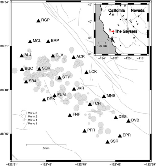
FIGURE 1. Geographic map of The Geysers geothermal field, California. Black triangles identify the seismic stations. Gray circles indicate the epicentral location of the earthquakes analyzed in the present study. Circle dimension is proportional to the event magnitude. Gray lines correspond to the known quaternary faults. The red square and the red arrow in the inset indicate the location of The Geysers geothermal field.

FIGURE 2

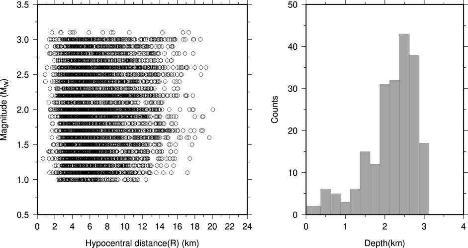
FIGURE 2. Scatter plot of the available strong-motion data in terms of Mw and R in the left-hand side plot and depth distribution of the analyzed earthquakes in the right-hand side plot.

FIGURE 3

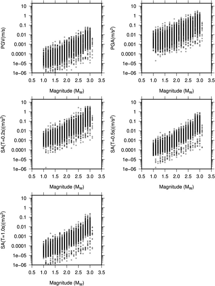
FIGURE 3. Peak ground velocity (PGV), peak ground acceleration (PGA), and spectral acceleration (SA) at 0.2, 0.5, and 1.0 s as function of moment magnitude in the earthquakes selected for the present study.

It is to be noted that for the largest portion of the earthquakes analyzed in this study, the Northern California Earthquake Data Center (NCEDC) catalog provides a duration magnitude M_D as a magnitude measure. However, we converted M_D into moment magnitudes M_w using a linear relationship by Douglas et al. (2013).

The epicentral location and seismic network configuration of earthquakes are shown in Figure 1. For convenience, we report the functional form of the GMM of Sharma et al. (2013), hereafter referred to as MOD3, that will be compared with the ANN model

${\mathit{log}}_{\mathit{10}}Y=a+b{M}_W+c{\mathit{log}}_{\mathit{10}}\sqrt{R^{\mathit{2}}+h^{\mathit{2}}}+es,(1)$

where the response variable Y is PGV, PGA, or SA(T) at T 0.2, 0.5, and 1.0 s, respectively. The model in Eq. 1 accounts for the source effect through the moment magnitude M_w and geometrical spreading through the hypocentral distance R. The h parameter is introduced to avoid unrealistically high values at short distances (e.g., Joyner and Boore, 1981), while the coefficient e represents the station/site effect. At each station, the dummy variable s is −1, 0, +1 depending on the mean value of the residuals distribution, when compared with the hypothesized zero-mean distribution by using the Z-test (Emolo et al., 2011; Sharma et al., 2013; Emolo et al., 2015). Readers can refer to Table 3 of Sharma et al. (2013) for the inferred s value at each station and for each response variable, while the coefficients a, b, c, h, and e of Eq. 1 are listed in Table 1 in the present work.

TABLE 1

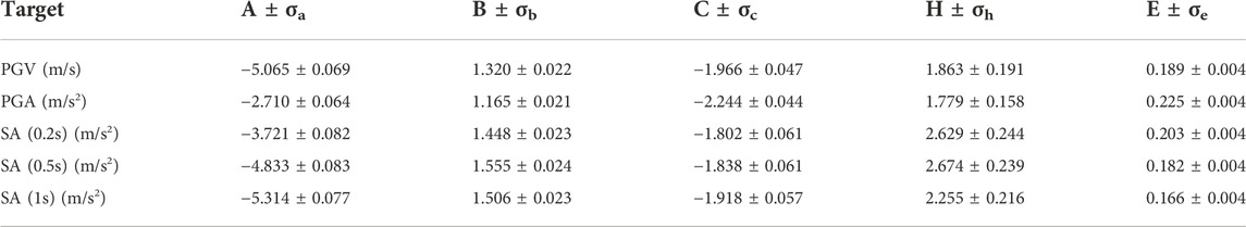
TABLE 1. Coefficients and uncertainties of the GMM reported in Eq. 1.

Proposed ANN-based ground motion models

The proposed model, inspired by the data-driven paradigm (Seydoux et al., 2020; Kuang et al., 2021), is constituted by the following steps: 1) preprocessing of the data features (in our case M_W, $R$ and s) by encoding or scaling in a suitable range; 2) the prediction by a feedforward multilayer perceptron (MLP); 3) rescaling of the prediction to the original target space. The preprocessing step is typically used to improve the convergence of the ML model (Han et al., 2012). First, we define how the data are preprocessed for both the input and the output and then how the MLP model is defined.

The preprocessing step is performed by taking into account the data type: M_W, $R$, and the targets ${\mathit{log}}_{10}Y$ are numeric, while s can be considered categorical. For this reason, the preprocessing of the feature $s$ consists of converting it to two new features, $\underset{\_}{s}=\left[s_{-1},s_1\right]$, with a one-hot encoding strategy, i.e., by using this following mapping: −1 becomes [1, 0.], 0 becomes [0, 0.], 1 becomes [0, 1.] (referred to as ${\varphi }_s$).

For the rescaling of the features and the target, we used the minmax scaling procedure: given a feature or target $x$, after computing the minimum value and the maximum value of $x$ in the considered dataset, the values of $x$ are linearly rescaled to a new prefixed range, most commonly between 0 and 1, i.e., such that the minimum value of $x$ is rescaled to the new minimum value in the prefixed range and the maximum value of $x$ is rescaled to the new maximum value in the range. This operation is also used by other data-driven approaches for the ground motion (Derras at al., 2014, Khosravikia and Clayton, 2021) and allows the training procedure of the considered model to stabilize (Han et al., 2012), but differently from the previous approaches, to strengthen the robustness of the methodology against the data leakage phenomenon, the considered dataset where to extract the minimum and the maximum values should be corresponding to the subset of the dataset where a data-driven model is fitted, i.e., the training set, not on the whole dataset (Kuhn & Johnson, 2019). Because of this, to avoid problems related to the ground motion parameter range in the training set being possibly smaller than the ones in the remaining data or in any new data, we ensure that the output range of the ANN-based ML model is larger than the scaled output interval, as described later. In order to keep the notation coherent, we denote with ${\varphi }_{M_w},{\varphi }_R,{\varphi }_Y$ the minmax function applied to the features $M_w$, $R$, and target $Y$, respectively.

An MLP model can be defined starting from a layer function $f:R^N\to R^M$, defined as in the following equation:

$f\left(v;W,b\right)=\sigma \left(Wv+b\right),(2)$

where the vector $W$ is called the weights matrix, $b$ is called the bias vector, and $\sigma :R^M\to R^M$ is the activation function. The MLP model $\psi$ can be defined as (Goodfellow et al., 2016

$\psi \left(x;\theta \right)=\left(f_{\mathit{1}}\odot f_{\mathit{2}}\odot ...\odot f_L\right)\left(x;\theta \right),(3)$

where L is the depth of the network, i.e., the number of layers, $f_j$ is a function as defined in Eq. 2 with parameters $W_j$ and $b_j$ and activation function ${\sigma }_j$, and $\theta =\left\{W_1,...,W_L,b_1,...,b_L\right\}$ are the parameters to estimate. The symbol $\odot$ denotes the composition operation between two functions, i.e., $\left(f\odot g\right)\left(x\right)=g\left(f\left(x\right)\right)$. The layers from $f_1$ to $f_{L-1}$ are named as hidden layers, and the last layer $f_L$ is named as the output layer. For our purpose, given that shallow models are known to be well-performing in the seismological context (Kong et al., 2019), the number of layers is constrained to be no more than 3, reducing considerably the model complexity. Moreover, in order to closely represent the neurological structure, all the activation functions except for the last one are the same. In our case, by using a grid search approach, whose criterion is explained in the subsection “Performance analysis and model validity,” we found that the best architecture is based on two hidden layers each made of 16 neurons, and the activation functions before the final layer are the sigmoid function $\sigma \left(x\right)=1/\left(1+e^{-x}\right)$ (which is also known as the log-sigmoid activation function in Derras et al., 2014) and as the last activation function the ranged version of the sigmoid function $\sigma \left(x;a,b\right)=\left(b-a\right)\sigma \left(x\right)+b$, with $a=-0.5$ and $b=1.5$, which has been possible with the scaling of the targets to [0, 1]. Also, $a$ and $b$ were chosen with a grid search, with this grid of choice (represented as pairs of $a$ and $b$): (−0.5, 1.5), (−1, 2), (−1.5, 2.5). These specific values are used to fix the center of the range to 0.5, as in the [0, 1] range scaling. Such a larger output range is explored to avoid that the predicted values stagnate at the two extremes of the scaled target interval. Such a problem can be avoided if the linear activation function is used, but we found it much less performing than the former approach. The architecture of the selected network is shown in Figure 4.

FIGURE 4

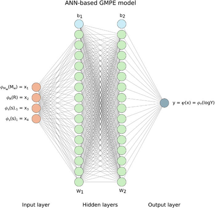
FIGURE 4. Proposed ANN architecture for the GMPE model. It is made of two hidden layers made of 16 neurons in each layer. W₁, W₂, b₁, and b₂ are the parameters from Eq. 3.

When we combine all the components together, the final formulation of the model used to estimate the response variables (i.e., PGV, PGA, or SA (T 0.2, 0.5, and 1.0 s) can be expressed in the following way:

${\mathit{log}}_{\mathit{10}}Y={{\varphi }_Y}^{-\mathit{1}}\left(\psi \left({\varphi }_{M_w}\left(M_W\right),{\varphi }_R\left(R\right),{\varphi }_s\left(s\right)\right)\right),(4)$

which is similar to the one present in Khosravikia et al. (2019), but without restricting the number of layers to 1, as such a configuration did not provide substantial results for this dataset.

For the training of this model, the strong-motion calibration dataset is randomly split into a training set made of 80% of the events, and a test set corresponding to the remaining events (in the deep learning community, the terms used for the splitted dataset is train-validation-test sets, as seen in Goodfellow et al. (2016); in this work, we adopt the convention train–test validation sets instead to avoid any confusion on the known notation “calibration dataset” for the fitting of the model and “validation dataset” for the evaluation of the performances; therefore, in our case, the “test set” is the set used to evaluate the generalization of the model in each training epoch and eventually stop the training earlier in case the loss value stops decreasing). The reason behind this strategy is due to the need to keep the within-event relations in all the samples belonging to the same event in either the training set or the test set, and therefore, reduce another source of data leakage, as also explained in (Khosravikia et al., 2019).

For the fitting of this model, we considered the family of stochastic gradient descent (SGD) methodologies (Goodfellow et al., 2016), which require three following steps: initialization, loss function, and optimization procedure. In the deep learning context, the weight initialization may have a strong influence on the convergence of the methodology; the same aspect is present for our ANN methodology, as we found by grid search that the best way to initialize the network weights was the random orthogonal initializers (Saxe et al., 2013). This methodology consists in generating randomly orthogonal weight matrix $W$ in Eq. 2 (i.e., such that $W^{T}W=I$), allowing the training procedure to extract only the mostly essential features from the input or from the output of the previous layer.

For the loss function, we used the following method:

$Loss\left(\widehat{y},y\right)=\alpha MSE\left(\widehat{y},y\right)+\beta RESSD\left(\widehat{y},y\right),(5)$

where $\alpha$ and $\beta$ are constant coefficients, $MSE$ is the mean square error, while $RESSD$ is defined as the following:

$RESSD\left(\widehat{y},y\right)=\frac{\mathit{1}}{N}{{\displaystyle \sum }}_{i=\mathit{1}}^N{\left(r_i-\underset{¯}{r}\right)}^{\mathit{2}}(6)$

With ${\widehat{y}}_i$ and $y_i$ the estimated target of the i-th sample of the considered dataset by the model and the corresponding original target, respectively, r_i = ln $y_i$- ln ${\widehat{y}}_i$ the residual of the i-th sample and $\underset{\_}{r}$ the mean value of $r_i$. The idea behind this loss function is that we need to take into account the variability of the targets in terms of the distribution of the residuals with respect to the features. This idea proved to be more helpful than using only the MSE, as in our tests, we found that $\alpha =1$ and $\beta =1.5$ gave the best results. Finally, we found that the best SGD methodology for this specific problem in terms of the evaluation metrics, as described in the subsection “Performance analysis and model validity,” is the Adam algorithm (Kingma and Ba, 2014) with a learning rate 0.1 and default parameters.

Performance analysis and model validity

We evaluated the prediction capability of the adopted model and compared it with MOD3 by using the following metrics: the total standard deviation (σ) and the two components of σ, the between-event standard deviation (τ) and the within-event standard deviation (ς), and finally the R² score. The formulation of the total standard deviation and its components are as follows:

$\sigma =\sqrt{\frac{{\displaystyle \sum }_{j=\mathit{1}}^E{\displaystyle \sum }_{i=\mathit{1}}^{N_j}{\left(r_{ij}-\overline{r}\right)}^{\mathit{2}}}{N-\mathit{1}}}(7)$

$\varsigma =\sqrt{\frac{{\displaystyle \sum }_{j=\mathit{1}}^E{\displaystyle \sum }_{i=\mathit{1}}^{N_j}{\left(r_{ij}-{\overline{r}}_j\right)}^{\mathit{2}}}{N-E}}(8)$

$\tau =\sqrt{{\sigma }^{\mathit{2}}-{\varsigma }^{\mathit{2}}}(9)$

where the residuals r_ij are defined as lnY^obs-lnY^pred, for event j and station i. N is the total number of stations, N_j is the total number of stations related to event j, E is number of earthquakes, $\underset{\_}{r}$ is the average residual for all the earthquake and all the stations, and ${\underset{\_}{r}}_j=\left({\displaystyle \sum }_{i=1}^{N_j}{r}_{ij}\right)/N_j$ is the average residual for event j computed for all the stations that have recorded the event (e.g., Douglas and Gehl, 2008). These formulations may differ from those in Sharma et al. (2013) because the computed values of sigma in Sharma et al. (2013) depend on the estimated coefficients through the nonlinear mixed-effect regression. In ML approaches, one of the most common metrics for regressive tasks is the root mean square error (RMSE), but it was not reported in this study, given that the difference between the values of RMSE and the values of σ ones are negligible in the results.

To take into account the possible prediction bias from how the ANN model weights are initialized and how the test set is randomly selected, the metrics are computed for five different runs of the fitting of the ANN model, where each run is characterized by a randomic splitting seed of the original dataset into the training and test set and the random initialization of the weights of the model. The resulting metrics are averaged, with their standard deviation computed to assess the variability of the predictions given by the model. The behavior of the loss function on both the training set and the test set with the variability of the runs in terms of the least number of epochs and the most number of epochs is illustrated in Supplementary Figure S1.

As for the search of the optimal hyperparameters of the ANN model, we used a grid search approach with the optimal criterion the minimization of the mean MSE from the k-fold cross-validation on the training set with k=5 applied in each run. In more details, in each run, the training dataset is split in k evenly divided subsets with the same splitting strategy based on the events described in the “Proposed ANN-based GMM” subsection, and then k ANN models are built with the fixed hyperparameters set from the grid and each of them is trained on one of the possible combinations of k-1 subsets and evaluated on the remaining subset. Due to the fact that the cross-validation is performed in each run with fixed seed, the obtained partitions from the split will differ in each run, making it possible to have an unbiased estimation of the model performance (Varma and Simon, 2006).

Comparison with the empirical ground motion models

We compare the ANN model with the empirical GMM of Sharma et al. (2013) by selecting ground-motion parameters for three distinct classes of magnitude, i.e., M_W ≤ 1.5, 1.5 < M_W < 2.5, and M_W ≥ 2.5. Both the models are plotted as a function of the hypocentral distance, for the magnitude value reported in each panel and without station/site effects (Figure 5). The most interesting result is that, while the empirical GMM is characterized by the same shape aside from the magnitude, the ANN model is characterized by distinct trends for each magnitude class. For example, the ANN model suggests trilinear amplitude decay with distance particularly for the lower-magnitude classes. These results also reflect into the residual distribution, which are defined as Res=lnY^obs-lnY^pred. In fact, as shown in Figure 6, the residuals as a function of the magnitude do not show any significant difference when the predictions are obtained by using the empirical GMM and the ANN model. However, it should be noted that both MOD3 and ANN models do not properly fit ground motion parameters relative to the large magnitude values ($M_W\ge 3.2)$. This is obviously due to the scarcity of the data in this specific magnitude range. As for the trend with the distance, Figure 7 suggests that the ANN provides slightly lower residuals at distances lower than 2 km for both PGA and PGV with respect to the GMM model.

FIGURE 5

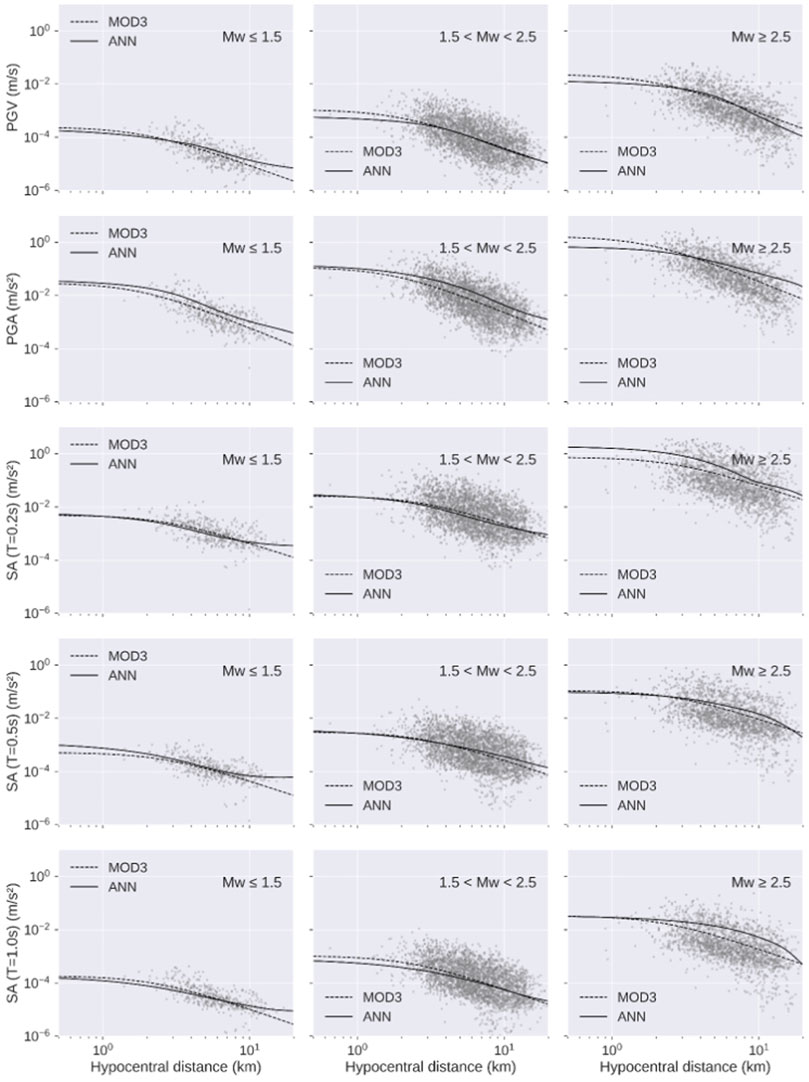
FIGURE 5. Empirical GMM (dashed line) and the DL model (continuous) plotted as function of the hypocentral distance for three classes of magnitude whose central value is reported in each panel. The dots represent the strong-motion observations. Peak ground motion parameters and response spectrum ordinates are colored according to the data density.

FIGURE 6

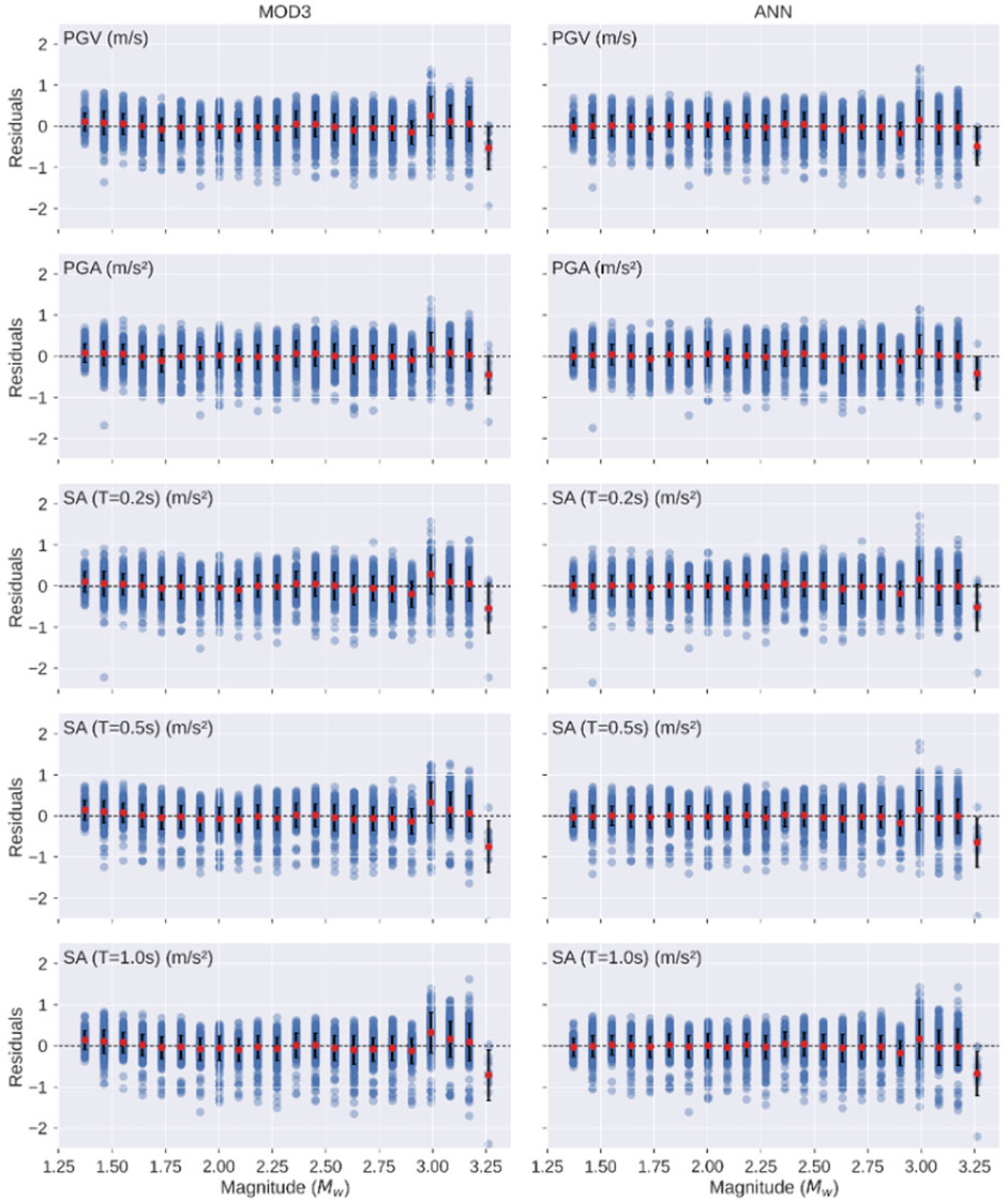
FIGURE 6. Residual plots with binned means (red dots) and standard deviation (vertical lines) relative to the magnitude for the models MOD3 and ANN. The dashed line is present to mark the zero-residual level.

FIGURE 7

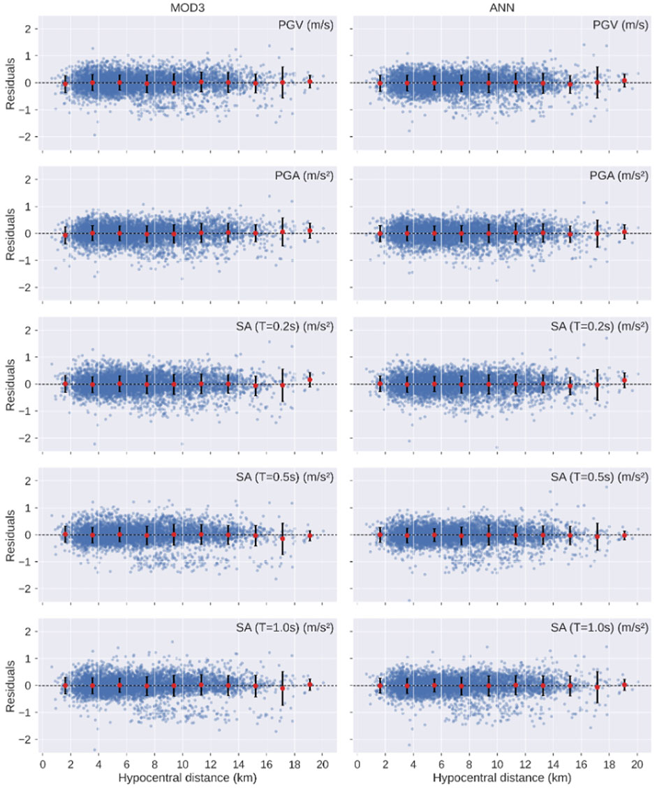
FIGURE 7. Residual plots with binned means (red dots) and standard deviation (vertical lines) relative to the hypocentral distance for the models MOD3 and ANN.

Furthermore, the ANN model shows a small increase in the predicted values at larger distances for small magnitude ($M_W\le 1.5)$, which is in contrast with the expected attenuation (i.e., geometrical spreading and anelastic attenuation). This can be due to the fact that, the ANN model being a data driven model, it tends to fit local data patterns rather than simply provide an average fitting. Indeed, the observed behavior is driven by the few points at distances larger than 10 km (Figure 5).

In order to quantitatively evaluate the differences between the two models, as reported in the previous section, we compute the coefficient of determination R², the total standard deviation, and its two components. The values obtained by using the ANN model are listed in Table 2 for each ground-motion parameter, which also contains the results for the empirical GMM. The coefficient R² provided by the ANN is higher than that provided by the GMM, indicating that the ANN explains a slightly larger proportion of the total variance. If we compare, the total standard deviation (σ) for the ANN model is 2%–5% lower (on the log scale) than that of the Sharma et al. (2013) GMM model. In particular, a larger reduction of up to 15% is observed in the inter-event component of the total standard deviation. As reported by Al Atki et al. (2010), the inter-events residual accounts for average seismic source effects (averaged over all azimuths) and is influenced by factors that are not captured by the inclusion of magnitude, style of faulting, and source depth. Among the factors, stress drop and variation of slip in space and time can be mentioned. Thus, the observed reduction of the inter-events residuals may suggest that the ANN model can account for differences in sources’ factors, but we cannot identify which is the dominant one.

TABLE 2

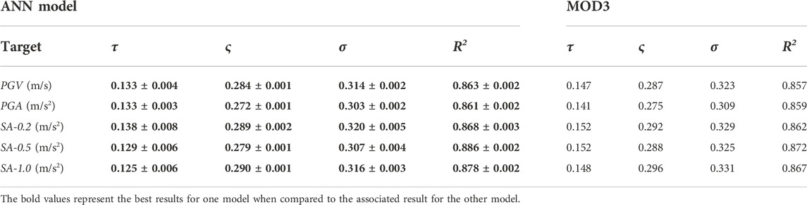
TABLE 2. Performance results of the proposed ANN model and MOD3 of Sharma et al. (2013) using the data set of The Geysers geothermal region. The results are expressed in terms of mean ± standard deviation for the ANN model. The best results are reported in bold.

To further verify the robustness of the proposed approach, as validation we used distinct data from the original dataset, containing 25 earthquakes recorded in the same area with magnitude ranging between 1.0 and 3.1 and distances ranging between 1.2 and 15.5 km (see Supplementary Figure S2). The results are shown in Supplementary Figures S3–S5, while the relative metrics are reported in Table 3. The results indicate that the trends are quite similar to those obtained from the calibration dataset. In particular, due to the data distribution, both GMPE and the proposed ANN model show higher residuals at larger magnitude values (Mw > 2.5). This is also confirmed by the metrics, which indicate that, compared with the results on the calibration dataset, both ANN and MOD3 report higher values of all the residual deviations and lower values of R². Nevertheless, the ANN outperforms MOD3 in all the metrics, except for the intra-event standard deviations for all the SA predictions. This can be likely due to the fact that in its present design, the ANN may be less effective in catching the differences between peak-ground motion parameters related to propagation path and local site conditions.

TABLE 3

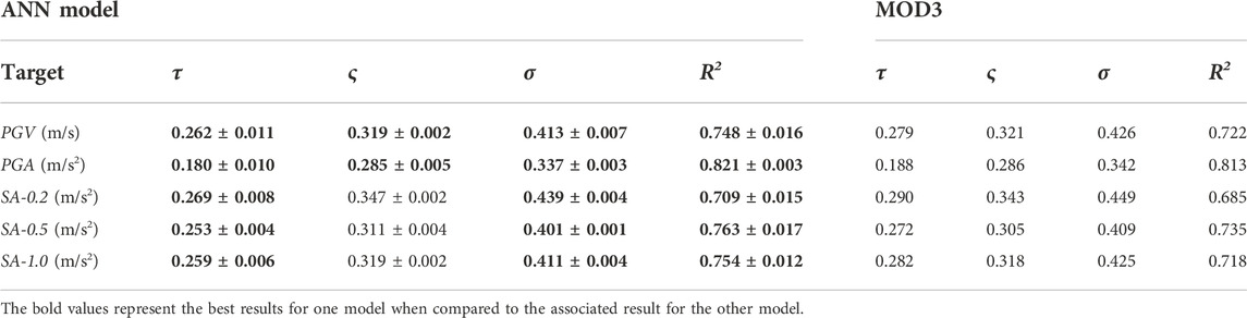
TABLE 3. Performance results with the proposed approach, compared with MOD3 of (Sharma et al., 2013) in the test data, reported in terms of mean ± standard deviation for the ANN model. The best results are reported in bold.

Since GMMs are key elements in seismic hazard, here, we show how the obtained ANN model and the associated standard error affect the calculation with respect to the empirical model. To perform this, we focus our attention to the conditional probability of exceeding a given peak ground motion value Ao, given the occurrence of an earthquake with magnitude M_W at a given distance R from a site of interest, that is, p [A>Ao|M_W,R] (Cornell, 1968; Reiter, 1990). As it is known, this probability is obtained from the GMM assuming that peak ground motion parameters are governed by a log-normal probability distribution with a mean value obtained from the ground motion prediction equation (e.g., Cornell 1968; Reiter, 1990; Budnitz et al., 1997; McGuire, 2004; Convertito and Herrero, 2004; Convertito et al., 2009). By using MOD3 of Sharma et al. (2013) and the ANN model obtained in the present study, we compute the exceedance probability (EP) curves shown in Figures 8, 9 for PGV and PGA, respectively. The results indicate that the differences between the EP curves for the two models do not show a unique behavior, but there is a dependence on the magnitude and distance values. Since both the models have constant (but different) total standard error, this behavior can be ascribed to the difference in the attenuation with distance. Moreover, in the case of the empirical model, the difference in the predicted values as a function of the magnitude is constant regardless of the distance; this is not true for the ANN model. This explains why the difference between the EP curves is not constant. For example, for M_W 3.0 and R = 1.0 km, the EP curve for the ANN model predicts lower exceedance probability values than the empirical model (Figures 8, 9). As for PGA, more important differences—up to three times—are evident in EP curves at 10 km distance and for all the three magnitude values. Finally, we compare the exceedance probability (EP) curves obtained from the two models with those computed from PGV- and PGA-recorded data. The observed EPs are shown in Figures 8, 9 as blue curves. We note that, given the real data distribution, in order to compute the observed EP, we selected a range of distances which contains the distance at which the EP curves have been obtained. As an example, for R=1 km, we used 0<R<3 km, for R=5 km 4.0<R<6.0 km, and for R=10 km 9<R<11 km. The results show that the observed EP almost for all distances and magnitude value is contained in the ±1 standard deviation curves of the empirical EP relative to ANN and is closer to the median curve of the ANN model with respect to the GMPE model. This suggests that in a future application of the two ground motion models in the framework of seismic hazard analysis, the ANN could provide more reliable results compared with the empirical GMM model.

FIGURE 8

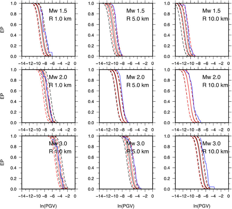
FIGURE 8. Exceedance probability curves (EP) for PGV. Black and red curves were obtained using MOD3 and ANN models, respectively. Continuous lines refer to the median value, while the dashed lines correspond to ±standard deviation. Each panel reports the selected magnitude and hypocentral distance value. The blue curves in each panel represent the observed EP obtained from the recorded PGVs.

FIGURE 9

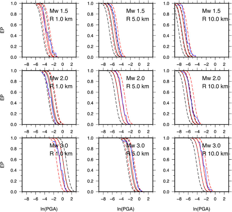
FIGURE 9. Same as Figure 8 but for PGA.

Conclusion

We implement an artificial neural network to model peak-ground motion parameters and spectral ordinates at three structural periods using seismic records from induced earthquakes in The Geysers geothermal region. We analyzed the data for the period September 2009 to November 2010. The same dataset has been previously used by Sharma et al. (2013) to infer empirical models by using the nonlinear mixed effect regression technique.

The proposed ANN is based on three main steps. First, preprocessing of the features, either by rescaling or by one-hot encoding (which is the case for the coefficient s); second, the prediction by a feedforward multi-perceptron layer (MLP) and finally a rescaling of the prediction to the original target space. Additionally, a modification to the loss function for the model training with the incorporation of the RESSD has been carried out to further penalize residual deviations of the seismic ground motion parameters, which helped in improving the residual scores in general.

The adopted data-driven approach suggests a magnitude scaling of the ground-motion parameters with distance. The ANN model is able to catch a trilinear dependence of such attenuation, which was not supported by the empirical model inferred from the same dataset. This is a very important feature when data show a high scattering as in the case of small magnitude-induced earthquakes. Interestingly, the ANN models, without any a priori assumption, also confirm the observed saturation effect with the distance modeled through the fictitious depth in the empirical model.

The obtained results suggest that the ANN model can be used for predicting strong ground motion parameters for the entire range of magnitude explored in this study, that is, (0.0, 3.3), but for magnitude lower than 1.5, the distance must be less than 10 km.

When looking at the exceedance probability, which plays a fundamental role in seismic hazard analysis, the obtained results demonstrate that the improvement in both the median ground motion estimates and the reduction of the total standard error result in a significant variation of the exceedance probability.

The results are thus promising and could be useful to refine seismic hazard results, particularly in the framework of induced earthquakes. Considering the flexibility in the component-wise structure of an ANN model, future works could focus on finding new functions and new training procedures which would not only improve the results but also add knowledge from the seismologic field. (Ji et al., 2021), (Sharma and Convertito, 2018)

Data availability statement

Publicly available datasets were analyzed in this study. These data can be found here: http://www.ncedc.org, network code BG. The data of the Lawrence Berkeley National Laboratory Geysers/Calpine seismic network have been retrieved from the Northern California Earthquake Data Center (NCEDC; network code BG; http://www.ncedc.org, last accessed January 2012). Figures 1–3, 8, 9 have been generated with the Generic Mapping Tools (GMT; Wessel and Smith, 1991). Figure 4 has been made with theNN-SVG online tool (LeNail, 2019). Figures 5–7 were generated with matplotlib and seaborn libraries (Hunter, 2017; Waskom, 2021). The ANN methodology was built in Python using as framework PyTorch (Paszke et al., 2019). The code is available upon reasonable request.

Author contributions

FP and VC coordinated the research and the design of the NN model. EP and NS designed the NN model and conducted the experiments. All the authors reviewed the manuscript.

Funding

This work has been designed and developed under the “PON Ricerca e Innovazione 2014-2020”– Dottorati innovativi con caratterizzazione industriale XXXVI Ciclo, Fondo per lo Sviluppo e la Coesione, code DOT1318347, CUP E63D20002530006.

This study has been also supported by PRIN-2017 MATISSE Project, No. 20177EPPN2, funded by the Italian Ministry of Education and Research.

Acknowledgments

NS is also thankful to the support provided by CSIR-National Geophysical Research Institute, Hyderabad, India.

Conflict of interest

The authors declare that the research was conducted in the absence of any commercial or financial relationships that could be construed as a potential conflict of interest.

The reviewer MP declared a shared affiliation with the author(s) EP and FP to the handling editor at the time of review.

Publisher’s note

All claims expressed in this article are solely those of the authors and do not necessarily represent those of their affiliated organizations, or those of the publisher, the editors, and the reviewers. Any product that may be evaluated in this article, or claim that may be made by its manufacturer, is not guaranteed or endorsed by the publisher.

Supplementary material

The Supplementary Material for this article can be found online at: https://www.frontiersin.org/articles/10.3389/feart.2022.917608/full#supplementary-material

References

Ahmed, S. A., Lisa, M., Hussain, M., and Khan, Z. U. (1274). Supervised machine learning for predicting shear sonic log (DTS) and volumes of petrophysical and elastic attributes, Kadawari gas filed, Pakistan. Front. Earth Sci.

Google Scholar

Arrieta, A. B., Díaz-Rodríguez, N., Del Ser, J., Bennetot, A., Tabik, S., Barbado, A., et al. (2020). Explainable Artificial Intelligence (XAI): Concepts, taxonomies, opportunities and challenges toward responsible AI. Inf. Fusion 58, 82–115. doi:10.1016/j.inffus.2019.12.012

CrossRef Full Text | Google Scholar

Atik, A. L., Abrahamson, N. A., Bommer, J. J., Scherbaum, F., Cotton, F., and Kuehn, N. (2010). The variability of ground-motion prediction models and its components. Seismol. Res. Lett. 81, 794–801. doi:10.1785/gssrl.81.5.794

CrossRef Full Text | Google Scholar

Bachmann, C. E., Wiemer, S., Woessner, J., and Hainzl, S. (2011). Statistical analysis of the induced basel 2006 earthquake sequence: Introducing a probability-based monitoring approach for enhanced geothermal systems. Geophys. J. Int. 186 (2), 793–807. doi:10.1111/j.1365-246X.2011.05068.x

CrossRef Full Text | Google Scholar

Bindi, D., Pacor, F., Luzi, L., Puglia, R., Massa, M., Ameri, G., et al. (2011). Ground motion prediction equations derived from the Italian strong motion database. Bull. Earthq. Eng. 9, 1899–1920. doi:10.1007/s10518-011-9313-z

CrossRef Full Text | Google Scholar

Bommer, J. J., Oates, S., Cepeda, J. M., Lindholm, C., Bird, J., Torres, R., et al. (2006). Control of hazard due to seismicity induced by a hot fractured rock geothermal project. Eng. Geol. 83, 287–306. doi:10.1016/j.enggeo.2005.11.002

CrossRef Full Text | Google Scholar

Boore, D. M., and Atkinson, G. M. (2008). Ground-motion prediction equations for the average horizontal component of PGA, PGV, and 5%-damped PSA at spectral periods between 0.01 s and 10.0 s. Earthq. Spectra 24 (1), 99–138. doi:10.1193/1.2830434

CrossRef Full Text | Google Scholar

Convertito, V., and Herrero, A. (2004). Influence of focal mechanism in probabilistic seismic hazard analysis. Bull. Seismol. Soc. Am. 94 (6), 2124–2136. doi:10.1785/0120040036

CrossRef Full Text | Google Scholar

Convertito, V., Iervolino, I., and Herrero, A. (2009). Importance of mapping design earthquakes: Insights for the southern apennines, Italy. Bull. Seismol. Soc. Am. 99, 2979–2991. doi:10.1785/0120080272

CrossRef Full Text | Google Scholar

Convertito, V., Maercklin, N., Sharma, N., and Zollo, A. (2012). From induced seismicity to direct time-dependent seismic hazard. Bull. Seismol. Soc. Am. 102 (6), 2563–2573. doi:10.1785/0120120036

CrossRef Full Text | Google Scholar

Cornell, C. A. (1968). Engineering seismic risk analysis. Bull. Seismol. Soc. Am. 58, 1583–1606. doi:10.1785/bssa0580051583

CrossRef Full Text | Google Scholar

Cybenko, G. (1989). Approximation by superpositions of a sigmoidal function. Math. Control Signal. Syst. 2 (4), 303–314. doi:10.1007/bf02551274

CrossRef Full Text | Google Scholar

Derras, B., Bard, P. Y., and Cotton, F. (2014). Towards fully data driven ground-motion prediction models for Europe. Bull. Earthq. Eng. 12 (1), 495–516. doi:10.1007/s10518-013-9481-0

CrossRef Full Text | Google Scholar

Dhanya, J., and Raghukanth, S. T. G. (2018). Ground motion prediction model using artificial neural network. Pure Appl. Geophys. 175, 1035–1064. doi:10.1007/s00024-017-1751-3

CrossRef Full Text | Google Scholar

Douglas, J., and Aochi, H. (2008). A Survey of techniques for predicting earthquake ground motions for engineering purposes. Surv. Geophys. 29, 187–220. doi:10.1007/s10712-008-9046-y

CrossRef Full Text | Google Scholar

Douglas, J. (2003). Earthquake ground motion estimation using strong motion records: A review of equations for the estimation of peak ground acceleration and response spectral ordinates. Earth. Sci. Rev. 61 (1), 43–104. doi:10.1016/s0012-8252(02)00112-5

CrossRef Full Text | Google Scholar

Douglas, J., Edwards, B., Convertito, V., Sharma, N., Tramelli, A., Kraaijpoel, D., et al. (2013). Predicting ground motion from induced earthquakes in geothermal areas. Bull. Seismol. Soc. Am. 103 (3), 1875–1897. doi:10.1785/0120120197

CrossRef Full Text | Google Scholar

Douglas, J., and Edwards, B. (2016). Recent and future developments in earthquake ground motion estimation. Earth. Sci. Rev. 160, 203–219. doi:10.1016/j.earscirev.2016.07.005

CrossRef Full Text | Google Scholar

Douglas, J., and Gehl, P. (2008). Investigating strong ground-motion variability using analysis of variance and two-way-fit plots. Bull. Earthq. Eng. 6, 389–405. doi:10.1007/s10518-008-9063-8

CrossRef Full Text | Google Scholar

Draper, N. R., and Smith, H. (1998)., 326. John Wiley & Sons. Applied regression analysis.

Emolo, A., Convertito, V., and Cantore, L. (2011). Ground-motion predictive equations for low-magnitude earthquakes in the Campania-Lucania area, southern Italy. J. Geophys. Eng. 8, 46–60. doi:10.1088/1742-2132/8/1/007

CrossRef Full Text | Google Scholar

Emolo, A., Sharma, N., Festa, G., Zollo, A., Convertito, V., Park, J. H., et al. (2015). Ground-motion prediction equations for South Korea Peninsula. Bull. Seismol. Soc. Am. 105 (5), 2625–2640. doi:10.1785/0120140296

CrossRef Full Text | Google Scholar

Esteva, L., and Rosenblueth, E. (1964). “Espectios de temblores a distancias moderadas y grandes,” in Proceedings of the society of Mexican engineering seismologists Chilean conference on seismology and earthquake engineering (Chile: University of Chile).

Google Scholar

Goodfellow, I., Bengio, Y., and Courville, A. (2016). Deep learning. MIT press.

Google Scholar

Han, J., Pei, J., and Kamber, M. (2012). Data mining: Concepts and techniques. Amsterdam: Elsevier.

Google Scholar

Hunter, J. D. (2007). Matplotlib: A 2D graphics environment. Comput. Sci. Eng. 9 (3), 90–95. doi:10.1109/mcse.2007.55

CrossRef Full Text | Google Scholar

Ji, D., Li, C., Zhai, C., Dong, Y., Katsanos, E. I., and Wang, W. (2021). Prediction of ground-motion parameters for the NGA-west2 database using refined second-order deep neural networks. Bull. Seismol. Soc. Am. 111 (6), 3278–3296. doi:10.1785/0120200388

CrossRef Full Text | Google Scholar

Joyner, W. B., and Boore, D. M. (1981). Peak horizontal acceleration and velocity from strong-motion records including records from the 197 9 imperial valley, California, earthquake. Bull. Seismol. Soc. Am. 71, 2011–2038. doi:10.1785/bssa0710062011

CrossRef Full Text | Google Scholar

Khosravikia, F., and Clayton, P. (2021). Machine learning in ground motion prediction. Comput. Geosciences 148, 104700. doi:10.1016/j.cageo.2021.104700

CrossRef Full Text | Google Scholar

Khosravikia, F., Clayton, P., and Nagy, Z. (2019). Artificial neural network-based framework for developing ground-motion models for natural and induced earthquakes in Oklahoma, Kansas, and Texas. Seismol. Res. Lett. 90 (2A), 604–613. doi:10.1785/0220180218

CrossRef Full Text | Google Scholar

Kingma, D. P., and Ba, J. (2014). Adam: A method for stochastic optimization. arXiv preprint arXiv:1412.6980.

Google Scholar

Kong, Q., Trugman, D. T., Ross, Z. E., Bianco, M. J., Meade, B. J., and Gerstoft, P. (2019). Machine learning in seismology: Turning data into insights. Seismol. Res. Lett. 90 (1), 3–14. doi:10.1785/0220180259

CrossRef Full Text | Google Scholar

Kuang, W., Yuan, C., and Zhang, J. (2021). Real-time determination of earthquake focal mechanism via deep learning. Nat. Commun. 12, 1432. doi:10.1038/s41467-021-21670-x

PubMed Abstract | CrossRef Full Text | Google Scholar

Kubo, H., Kunugi, T., Suzuki, W., Suzuki, S., and Aoi, S. (2020). Hybrid predictor for ground-motion intensity with machine learning and conventional ground motion prediction equation. Sci. Rep. 10, 11871. doi:10.1038/s41598-020-68630-x

PubMed Abstract | CrossRef Full Text | Google Scholar

Kuhn, M., and Johnson, K. (2019). Feature engineering and selection: A practical approach for predictive models. Boca Raton, FL: CRC Press.

Google Scholar

LeNail, A. (2019). NN-SVG: Publication-Ready neural network architecture schematics. J. Open Source Softw. 4 (33), 747. doi:10.21105/joss.00747

CrossRef Full Text | Google Scholar

Loyola-González, O. (2019). Black-box vs. White-box: Understanding their advantages and weaknesses from a practical point of view. IEEE Access 7, 154096–154113. doi:10.1109/ACCESS.2019.2949286

CrossRef Full Text | Google Scholar

Okazaki, T., Nobuyuki, M., Fujiwara, H., and Ueda, N. (2021). ​​Monotonic neural network for ground-motion predictions to avoid overfitting to recorded sites. Seismol. Res. Lett. 92 (6), 3552–3564. doi:10.1785/0220210099

CrossRef Full Text | Google Scholar

Paszke, A., Gross, S., Massa, F., Lerer, A., Bradbury, J., Chanan, G., and Chintala, S. (2019). Pytorch: An imperative style, high-performance deep learning library. Adv. Neural Inf. Process. Syst. 32, 8026–8037.

Google Scholar

PicozziOthParolaiBindiDe Landro, M. A. S. D. G., Amoroso, O., and Bindi, D. (2017). Accurate estimation of seismic source parameters of induced seismicity by a combined approach of generalized inversion and genetic algorithm: Application to the Geysers geothermal area, California. J. Geophys. Res. Solid Earth 122, 3916–3933. doi:10.1002/2016JB013690

CrossRef Full Text | Google Scholar

Reiter, L. (1990). Earthquake hazard analysis. New York: Columbia University Press, 254.

Google Scholar

Sabetta, F., and Pugliese, A. (1996). Estimation of response spectra and simulation of nonstationary earthquake ground motions. Bull. Seismol. Soc. Am. 86, 337–352.

Google Scholar

Saxe, A. M., McClelland, J. L., and Ganguli, S. (2013). Exact solutions to the nonlinear dynamics of learning in deep linear neural networks. https://arxiv.org/abs/1312.6120.

Google Scholar

Seydoux, L., Balestriero, R., Poli, P., Hoop, M. d., Campillo, M., and Baraniuk, R. (2020). Clustering earthquake signals and background noises in continuous seismic data with unsupervised deep learning. Nat. Commun. 11, 3972. doi:10.1038/s41467-020-17841-x

PubMed Abstract | CrossRef Full Text | Google Scholar

Sharma, N., Convertito, V., Maercklin, N., and Zollo, A. (2013). Ground-motion prediction equations for the Geysers geothermal area based on induced seismicity records. Bull. Seismol. Soc. Am. 103 (1), 117–130. doi:10.1785/0120120138

CrossRef Full Text | Google Scholar

Sharma, N., and Convertito, V. (2018). Update, comparison, and interpretation of the ground-motion prediction equation for “the Geysers” geothermal area in the light of new data. Bull. Seismol. Soc. Am. 108 (6), 3645–3655. doi:10.1785/0120170350

CrossRef Full Text | Google Scholar

Strasser, F. O., Abrahamson, N. A., and Bommer, J. J. (2009). Sigma: Issues, insights, and challenges. Seismol. Res. Lett. 80, 40–56. doi:10.1785/gssrl.80.1.40

CrossRef Full Text | Google Scholar

Van Eck, T., Goutbeek, F., Haak, H., and Dost, B. (2006). Seismic hazard due to small-magnitude, shallow-source, induced earthquakes in The Netherlands. Eng. Geol. 87, 105–121. doi:10.1016/j.enggeo.2006.06.005

CrossRef Full Text | Google Scholar

Varma, S., and Simon, R. (2006). Bias in error estimation when using cross-validation for model selection. BMC Bioinforma. 7 (1), 91–98. doi:10.1186/1471-2105-7-91

PubMed Abstract | CrossRef Full Text | Google Scholar

Velasco Herrera, V. M., Rossello, E. A., Orgeira, M. J., Arioni, L., Soon, W., Velasco, G., et al. (2022). Long-term forecasting of strong earthquakes in north America, south America, Japan, southern China and northern India with machine learning. Front. Earth Sci. (Lausanne). 10, 905792. doi:10.3389/feart.2022.905792

CrossRef Full Text | Google Scholar

Waskom, M. L. (2021). Seaborn: Statistical data visualization. J. Open Source Softw. 6 (60), 3021. doi:10.21105/joss.03021

CrossRef Full Text | Google Scholar

Wessel, P., and Smith, W. H. F. (1991). Free software helps map and display data. Eos Trans. AGU. 72, 441–446. doi:10.1029/90eo00319

CrossRef Full Text | Google Scholar