Spatial and Temporal Variability of Bed Exchange Characteristics of Fine Sediments From the Weser Estuary

Sedimentation of fine-grained sediments in estuaries is a natural physical phenomenon influenced by biogeochemical processes. In the estuarine turbidity maximum (ETM), enhanced net deposition of sediments is observed even in areas with higher hydrodynamic exposure, such as the navigational channel. Maintenance dredging is a common method to maintain the navigational channel, which requires large financial effort and has potential negative impacts on the environment. Research at the Institute for River and Coastal Engineering addresses the challenge of understanding the processes leading to net sedimentation and accumulation in estuarine navigational channels in reach of the ETM. In this contribution, investigations of bed exchange properties of estuarine cohesive sediments conducted in field and laboratory studies are presented. The results provide rarely available and estuary-specific parameters characterizing sediment transport, mainly related to erosion processes. By performing field campaigns within the ETM of the Weser estuary, cores of freshly deposited sediments have been sampled from two sites (Blexer Bogen and Nordenham) along the center of the navigational channel. Sediment characteristics (grain size distribution, water content, loss on ignition, density profiles) have been derived, and the erodibility of the deposits is investigated both quasi in situ and in the laboratory using an erosion microcosm system. Erodibility experiments are run in a closed system so sediment concentration above the lutocline increases during the experiment. This is a unique feature of this study, and it is expected to produce more natural characteristics of net erosion. By proving the reproducibility of the natural structure of the deposited sediments (stratification and density profiles) in the laboratory, systematic studies for analyzing the sensitivity of determined parameters (shear stresses and erosion rates) to varying environmental conditions (settling conditions and density) could be performed. Temporal development of suspended sediment concentration and erosion rates is the main result of the erodibility experiments, from which we derive bandwidths for erosion parameters, like floc erosion rate, critical shear for floc erosion, and critical shear for mass erosion.

1 Introduction

Fine sediment transport plays a significant role in the marine environment, making a detailed understanding and capable modeling approaches of transport processes crucial for the strategic maintenance of estuaries. While the transport of non-cohesive sediment is understood reasonably well, the depiction and prediction of cohesive sediment transport are still a challenge because of their complex composition of inorganic minerals and organic material (Grabowski et al., 2011). Particle mixtures are referred to as cohesive sediments when they exhibit intrinsic cohesion (Winterwerp et al., 2021), which is the case when a mixture of fine sediments (fine sand, silt, and clay) exceeds a critical threshold for clay minerals, often reported to be 10% (van Rijn, 1993; Grabowski et al., 2011). Because almost all processes defining the properties of cohesive sediments vary with time and location, derived parameters for process description are sediment- and estuary-specific. When cohesion is dominant, particles are interconnected, forming flocs and aggregates, resulting in transport dynamics that are significantly different from non-cohesive sediment transport. Affected by tidal asymmetry, stratification, and estuarine circulation, suspended cohesive sediments tend to retain and accumulate in estuaries, resulting in a zone of relatively high concentration of suspended sediments, the estuarine turbidity maximum (ETM). The ETM accounts for the main sediment deposition in many systems, while the location and extent of the ETM are predominantly affected by river discharge and the tidal cycle (Grabemann, 1992). Anthropogenic impacts, e.g., the deepening of waterways to enhance navigability, have the potential to cause intensified sedimentation and deposition because tidal asymmetry may increase. Even in the deeper navigational channel, where high flow velocities may support sediment transport and erosion, partly intensive net sedimentation and accumulation can be observed with a resulting formation of temporary deposits of high concentrated mud suspensions (HCMS). Depending on the conditions, HCMS can occur either in a stationary or mobile state, the extent of which varies greatly in space and time. Maintenance dredging is a common method of preserving the essential water depths for navigability but requires high financial effort and has potential negative impacts on the environment. Against this background, research at the Institute for River and Coastal Engineering (IWB) of the Hamburg University of Technology (TUHH) is carried out to improve the understanding of bed exchange processes in the ETM exemplary for the Weser estuary.

In this study, natural sediments gathered from the navigational channel of the Weser estuary within the ETM are investigated. Determining the characteristics of erodibility is one major aspect of experiments undertaken. Sediments are investigated in two different states. First, mostly undisturbed samples containing natural sediments are characterized in field trips. Second, sediment characteristics are investigated by generating representative samples consisting of nature-like density profiles, salinity, and composition. Being the second-largest German estuary, the Weser discharges into the North Sea, like the other two major German estuaries of Elbe and Ems. All of the mentioned estuaries are facing similar challenges in fine sediment transport. The Weser is divided into different sections: The Upper Weser originates in Hann. Münden, where the headwaters of the Werra and Fulda rivers converge. The Middle Weser runs between Minden and Bremen, and the Lower and Outer Weser mark the tide-influenced area. While multiple definitions exist, here the Weser estuary and its kilometry is defined from the head at the tidal weir in Bremen-Hemelingen (def. as Weser-km 0), which marks the artificial tidal limit (Lange et al., 2008). Having a tidal range roughly between 3 m (Outer Weser) to 4 m (Bremen) and, as of today, a bottom at −11 m NHN in the navigational channel up to Blexen (Weser-km 65) and −16 m NHN further seawards, the Weser estuary is classified as mesotidal and hypersynchronical (Grabemann, 1992; Kösters et al., 2018; Hesse 2020). In general, deposited sediments reduce in size along the Weser from its origin to its mouth. In the Upper Weser, rubble sediment, in the Middle Weser, gravel, and in the Lower and Outer Weser, medium and fine sand are dominating most parts. Due to tidal dynamics and freshwater discharge, bed forms like dunes and ripples appear in the Lower Weser until Nordenham (NH, Weser-km 55). In the mixing zone of freshwater and seawater, density gradients lead to gravitational circulation and contribute to a resulting residual import of fine sediments. An ETM is formed, causing high sedimentation rates of up to 5 cm/d (internal analysis of echo sounder data), depending on several influencing factors, e.g., freshwater discharge, temperature, salinity, and sediment availability. In the ETM, suspended sediment concentrations (SSCs) of 300–600 mg/L in the water column and up to 2000 mg/L near the bottom are observed regularly (Lange et al., 2008). Multiple processes of deepening of the navigational channel from the past has affected the tidal symmetry, e.g., causing increased flood current velocities. Because of the resulting net sediment import, large sedimentation and deposition rates are noted. The resulting accumulation of sediments intensifies the challenge of keeping the main channel navigable. With frequent measurement campaigns conducted by the Federal Waterways and Shipping Administration (WSV), changes in bathymetry are surveyed using multibeam echo sounders (MBES). On the basis of the MBES results, maintenance dredging volumes are commissioned. In the range of km 55 of the Weser near NH to km 65 near Blexen, which is the major hotspot of dredging activity and the focus area of this research work (see Figure 1), 0.5–2 million cubic meters are dredged on a yearly base (Eberle, 2014). Because dredging activities require investments of 8–18 Mio. €/year and each displacement of dredged material has a potential ecological impact in the Lower and Outer Weser, it becomes clear that optimized maintenance resulting from an improved understanding of estuarine processes is of true value for the environment, citizens, authorities, and other stakeholders.

FIGURE 1

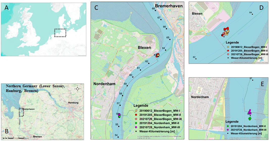
FIGURE 1. Location of German estuaries in Europe (A), Weser and Elbe estuaries located in northern Germany (B), sampling sites in the estuarine turbidity zone of the Weser estuary (C), and a close view at Blexer Bogen (D) and Nordenham (E); maps by ©OpenStreetMap.

In the following paragraph, a hypothesis is formulated as to how the accumulation of cohesive sediments in the navigation channel of the Weser occurs. Echo sounder data indicate that sedimentation and deposition within the ETM dominate in phases of low flow velocities. Depositing flocs and particles form a layered structure above the (dense) bed of the waterbody of several decimeters up to meters in height (Papenmeier et al., 2013; Becker et al., 2018). This structure forms a fresh layer of mobile benthic suspension with initial densities in the range of ρ = 1,050 kg/m³, being well below the gelling point. Depending on the conditions during the formation of a mud layer and its state of consolidation, a sediment is composed of different percentages of sand, silt, and clay. If a mud layer is formed naturally due to sedimentation in phases of low velocities, differential settling likely leads to the segregation of particles (Torfs et al., 1996). As a result, one will find higher percentages of silt and clay in the upper part and higher sand contents in the lower part of the upmost sediment layer above the bed. The upper part of a freshly deposited layer may be eroded during the adjacent flood or ebb phase, while the lower part is affected by reduced shear stresses and will thus be able to increase its density over one to several tides. The lower part of that layer, now forming stationary fluid mud, is, on the one hand, more resilient to erosion and, on the other hand, protected against erosion by the concentrated benthic suspension (CBS) above. The CBS might be regenerated with every tide. In the stationary fluid mud layer, concentrations exceed structural density (also called the gelling point/concentration), meaning that particles and flocs form a coherent structure (van Rijn, 2016). At structural density, effective stresses start to emerge when expelled water reduces excess pore pressure. This indicates the beginning of the consolidation process. The transition between settling and consolidation is, for example, characterized by its vertical velocities. Settling velocities w_s are well above the rate of consolidation w_c (approx. by an order of magnitude), although both parameters characterize the process of vertical reduction of the suspension layer. In this way, during each phase of slack water, deposits accumulate near the bottom, forming a consolidated and stratified bed over time. Well-mixed, homogeneous sediment beds are rare in nature (van Rijn, 2020), but when it comes to dredging activities, homogeneous and stationary fluid mud layers might be formed without being affected by differential settling beforehand. Hence, dredging removes sediments, but the remaining sediments might be homogenized, forming a layer of stationary mud. This results in a resistive layer supporting the consolidation of fresh sediments. The mentioned type of bed formation is even expected to occur in the center of a tidal channel with relatively high flow velocities. With and without dredging inflluences, stratified and non-stratified suspensions have been observed in the Weser estuary throughout the field campaigns.

According to the current state-of-the-art, processes of fine sediment transport are replicated more or less accurately using morphodynamical-numerical modeling techniques. Morphodynamical-numerical models enable a process-based simulation of dynamics on a large spatial and temporal scale, allowing for impact studies of anthropogenic intervention and helping to understand the effect of several mechanisms consistently. Nevertheless, the underlying processes of those models are increasingly physically based, but major processes like the bed exchange processes are still based on empirical relationships. The parameters required for these approaches have to be derived by sensitivity studies in the laboratory and/or by intensive on-site measurement campaigns. In this context, erosion of cohesive sediments is a major mechanism that still needs empirical estimation of parameters to represent their erodibility properly. Investigation on the erosion behavior of sand-only deposits, on the one hand, and mud-only deposits, on the other hand, has been conducted for several decades. While the relationship between given flow conditions and the movement of sand particles can be described reasonably well with references from Shields (1936), it remains difficult to predict the behavior of mud-only, and especially sand–mud, mixtures because of interparticle forces, leading to transport properties depending on several further factors besides gravity (e.g., sand to clay ratio, concentration/density, consolidation and its history, organic matter content and type, temperature, salinity, sodium adsorption ratio, and pH). Those factors underlie a huge variability on different spatial and time scales, especially in estuaries (Winterwerp and van Kesteren, 2004). So far, no generally valid relation to describe bed exchange processes could be established using only physically based formulations (van Rijn, 2020).

However, several authors have provided empirical relationships to describe the erosion behavior of muddy sediments (Partheniades, 1965; Parchure und Mehta, 1985; Kranenburg und Winterwerp, 1997; Krishnappan, 2000; Whitehouse et al., 2000; Sanford und Maa, 2001; Schweim, 2005; Mengual et al., 2017; Krishnappan et al., 2020; Chen et al., 2021), mostly by relating applied shear stress to resulting erosion rates, but only a few models have made their way into engineering and modeling practice (Partheniades, 1965; Parchure und Mehta, 1985; Sanford und Maa, 2001). Models can be distinct by depth-dependent or depth-independent erosion resistance (summary in William et al., 2000). Erosion is observed to occur in different modes depending on the range of applied shear stress (Winterwerp and van Kesteren, 2004; Kombiadou und Krestenitis, 2013; van Rijn, 2020; Chen et al., 2021). At low shear stresses, single particles and flocs are eroded from locations of weak erosion resistance when sudden peaks (turbulence) in applied shear stress occur. This mode is called floc erosion. The erosion rate for floc erosion is observed to be approx. 10^–8–10^–4 kg/(m² s) (Schweim, 2005). When medium shear is applied, an intermediate stage of erosion, sometimes referred to as surface erosion, might occur, in which several layers of particles and flocs are mobilized (a failure of local networks). The transition between floc and surface erosion is smooth; hence, we do not make a distinction at this point in time. At higher shear, mass or bulk erosion dominates, eroding lumps or chunks of bed material. The erosion rate for mass erosion is observed to be approx. 10^–3–10^–1 kg/(m²/s) (van Rijn, 2020). Although it was proposed for homogeneous consolidated beds (constant in time and within the sediment), the “Partheniades law” (Partheniades, 1965) is used very commonly in modeling practice. The Partheniades law relates the applied shear to the erosion rate, which is the eroded mass per unit surface and unit time. In fact, erosion resistance depends on various factors, including sediment composition, porosity, and degree of consolidation (Kombiadou und Krestenitis, 2013). This means, in turn, that sediment deposits regularly are thought to have heterogeneous properties with depth and time. However, it is possible to argue that the composition of sediment deposits can be homogeneous over a limited depth to apply Partheniades law and use individual fitting parameters for depth (e.g., fresh fluid mud deposits). In the past, the Partheniades law was extended to become valid for depth-dependent erosion resistance:

$E=E_{0,mud}{\left(\frac{{\tau }_b}{{\tau }_{cr}(z)}-1\right)}^n, if {\tau }_b\ge {\tau }_{cr},(1)$

where E [kg/(m²s)] is the erosion rate, E_0,mud [kg/(m²s)] is an empirical erosion constant, τ_b[N/m²] is the applied shear , n is an empirical parameter, and τ_cr(z) [N/m²] is the depth-dependent critical shear for erosion. The simplicity of this model is most likely a major reason why the Partheniades law is used very commonly in modeling practice. Sanford and Maa (1985) proposed a relationship for more soft mud deposits, taking the state of consolidation and the depth-dependent density ρ(z) [kg/m³] at the sediment–water boundary into account:

$E=\beta \ast \rho \left(z\right)\ast \left({\tau }_b-{\tau }_{cr}\left(z\right)\right) if {\tau }_b\ge {\tau }_{cr},(2)$

where E [kg/(m²s)] is the erosion rate, τ_cr [N/m²] is the depth-dependent critical shear for erosion, τ_b [N/m²] is the applied shear, and β [m²s/kg] is the empirical fitting parameter. The difference of critical to applied shear is referred to as effective stress.

Parchure and Mehta (1985) proposed a relationship for soft mud deposits, assuming a constant floc erosion rate ε_f and depth-dependent erosion resistance τ_cr:

$\epsilon ={\epsilon }_f{e}^{\alpha {\left({\tau }_b-{\tau }_{cr}\left(z\right)\right)}^{nm}}, if {\tau }_b\ge {\tau }_{cr},(3)$

where ε [kg/(m²s)] is the erosion rate, ε_f [kg/(m²s)] is the floc erosion rate, τ_b [N/m²] is the applied shear, α [m/N^0,5] is an empirical parameter, and τ_cr(z) [N/m²] is the depth-dependent critical shear for erosion. The floc erosion rate ε_f appears to vary greatly for individual sediment deposits, with a range of 10^–4 to 10^–8 [kg/(m²s)], while α appears to range between 1 and 30 (Schweim, 2005). When focusing on bed exchange, sediment deposition has to be taken into account:

$D=C_S\ast w_S,(4)$

where D [kg/(m²s)] is the deposition flux, C_S [kg/m²] is the sediment concentration near the bed, and w_s [m/s] represents the mean settling velocity of sediment particles.

The research at IWB addresses the challenge of understanding the process leading to net sedimentation and accumulation in estuarine navigational channels by investigating rarely available information on the vertical transport and bed exchange properties of estuarine sediments in field and laboratory studies. The sediment samples are taken from the navigational channel of the Weser estuary. We provide estuary-specific transport parameterizations and adjusted bed exchange formulations to advance the representation of sediment transport processes in large-scale 3D morpho- and hydrodynamic-numerical models. This contribution focuses on results from investigating natural cohesive sediments with measurements conducted in the field and in laboratory experiments, mainly related to erosion processes. Erosion rates and critical shear for floc and mass erosion are derived for sediments from two locations. The influence of consolidation history and density is further investigated in sensitivity studies.

2 Materials and Methods

2.1 Field Campaigns

To examine the assumptions made in Section 1, natural sediments from the Weser estuary are collected during slack water within the ETM of the Weser at Weser-km 56 (NH) and Weser-km 63 (Blexer Bogen, BB). Field campaigns have been realized with regard to meeting the following requirements of sediment samples:

i) Undisturbed (almost)

ii) From the navigational channel within the ETM zone

iii) Collected during slack water (v ≤ 0.4 m/s) with upstream river discharge conditions of approx. Q ∼ 150 m³/s (late spring and autumn discharge, when sedimentation rates peak)

iv) Being ideally composed of a water layer, a soft mud layer of fresh deposits, and a consolidating/consolidated layer.

To meet these requirements, a sediment corer for collecting undisturbed sediment samples (of soft mobile mud as well as consolidated mud) from the center of the navigational channel has been developed at the Institute for River and Coastal Engineering (Patzke et al., 2019), see also Figure 2. The samples are collected in Plexiglas cylinders of 20-cm diameter and 1.2-m height. At the top, the corer is equipped with a pressure gauge to determine the sampling depth. The timespan for the sampling of a single cylinder (preparing, coring, releasing) using the corer is under 10 min.

FIGURE 2

FIGURE 2. Sediment corer developed at the Institute for River and Coastal Engineering.

Three campaigns, MW-I (06/2019), MW-II (12/2019), and MW-III (07/2021), have been conducted on the Weser, where a set of six sediment cores could be obtained during the estimated slack water period of 1 h. Each core receives a sample code in the format “site abbreviation-campaignnumber/corenumber-subsamplenumber.” Campaign numbers start at 0. For example, code “BB-01-03” describes the third subsample from the first core taken in BB during MW-I. Specific cores are subsampled, representing layers of about 5–10 cm. By measuring the density of homogenized subsamples, profiles of the near-bottom layers are generated. Information on size segregation in the top and bottom layers is provided by additionally using the subsamples to determine grain size distribution. The remaining sediment cores are used to observe settling behavior and to provide sediment material for further laboratory studies. In MW-III, two cores of each sampling site could be used to perform quasi in situ erosion experiments, providing information on the erodibility of naturally stratified and composed sediments.

2.2 Sample Preparation and Sediment Characterization

2.2.1 Sample Preparation for Laboratory Experiments

To perform experiments in the laboratory, natural sediments collected during the field campaigns are used to prepare representative samples. A sample is defined as a representative if it comprises both natural material including solids and organic phase as well, having nature-like density profiles close to the sediment–water interface where erosion processes are investigated. In practice, the best results could be achieved by first predefining an initial density/concentration that was observed in the field. Second, a fraction of natural sediments was taken from a core to generate a suspension of the predefined density. In case fluid mud with a homogeneous density profile was extracted from the river bed, the whole core was used to generate a representative suspension. Then, the suspension is homogenized at time t₀ exhibiting the initial density ρ₀. Those generated suspensions are called remolded samples. The density evolution within those suspensions is recorded to describe and parameterize consolidation processes and to relate the erosion process to the state of consolidation. When erodibility experiments are conducted, the experiment starts at specific time intervals between t₀ and t_start. In that way, the consolidation history is taken into account. The influence of density on erodibility is specifically investigated by varying the initial density ρ₀.

2.2.2 Sediment Characterization

The natural sediments are characterized by performing standard soil mechanical laboratory tests. Grain size distribution is obtained by performing a combined sieve and sedimentation analysis following the standardized procedure of DIN EN ISO 17892-4. Water content (WC) is derived following DIN EN ISO 17892-1, in which the samples have to be oven-dried at 105°C for 24 h and weighed before and after drying. To estimate the organic content, loss on ignition (LOI) tests are performed following DIN 18128.

Sediment characterization is performed as a sample average of five samples from NH and five samples from BB as well. At campaign MW-I, only site BB is approached and sample BB-01 is chosen for sediment characterization. At campaigns MW-II and MW-III, both sites are approached. Two cores from NH, NH-11 and NH-13, and one core from BB, BB-11, have been separated into subsamples during MW-II. At campaign MW-III, one sample from NH, NH-35, and one sample from BB, BB-36, are chosen for sediment characterization. In addition, the cores of NH-11, NH-13, NH-35, BB-01, BB-11, and BB-36 are divided into subsamples to derive depth-dependent sediment parameters. In total, information for 80 samples and subsamples is derived. A summary of the results is shown in Section 3.1 in Table 1 and Figure 7.

TABLE 1

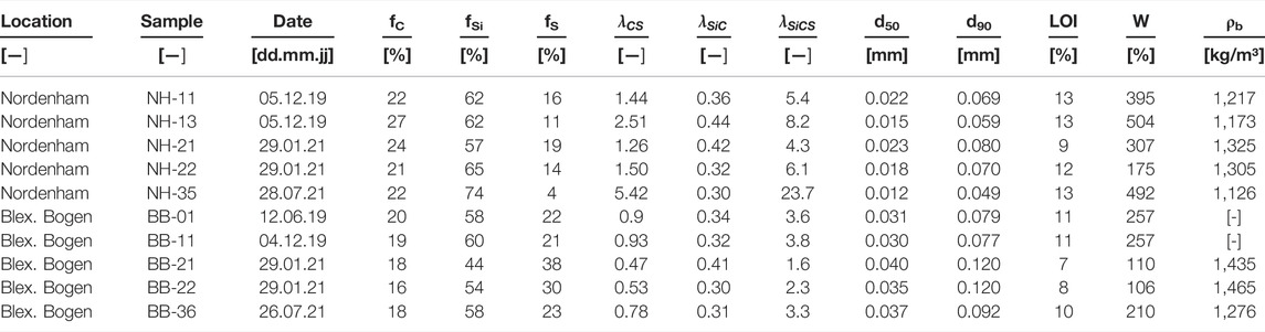
TABLE 1. Sediment properties: percentage breakdown of grain sizes (clay (f_C), silt (f_Si), sand (f_S), d₅₀, d₉₀), water content (W), loss on ignition (LOI), and bulk density (ρ_b) of sediment samples taken during field campaigns (MW-I, MW-II, MW-III) on the Weser estuary.

2.3 Density

Besides mean values for density and sedimentary composition (Table 1), density profiles are generated by applying two types of measurements. Density is measured using a suspension balance, and measurements are taken using the Anton Paar DMA 35 densimeter. Comparative measurements have proven the comparability of the measurement results with the two methods.

A. In the case of natural samples, density profiles are generated by subdividing the sample into layers of approximately 5 cm and measuring the mean density of each subsample using the suspension balance or the densimeter (depending on the sand content). In this way, a density profile is generated. After density measurements, the subsamples are still feasible for further investigation in soil mechanical tests (see Section 2.2).

B. In the case of remolded samples, a set of small pipes is used to extract tiny subsamples of approx. 5 ml at predefined depths using a syringe. The density of those subsamples is measured using the densimeter. To avoid the lower layers from being affected by the measurements, the procedure is undertaken from the top to the bottom of the sample. By restoring and remolding the sample after measuring a density profile, it becomes possible to investigate the temporal evolution of densities in the column. Besides the densities, the lutocline evolution is also recorded over time.

An internal analysis of dredging and echo-sounding data showed that the river discharge of 150 m³/s results in sedimentation foci predominantly in NH, but this also affects the BB area. Hence, differences in the density profiles from BB and NH may be explained by the position of the ETM being located rather nearer NH. The density of a sediment is seen as key information influencing erosion behavior.

2.4 Erosion

This study presents and discusses results from erodibility experiments performed quasi in situ and in the laboratory. Sediment cores taken from the Weser estuary are either preserved in natural stratification or being remolded to provide controlled initial conditions. Three types of erosion experiments have been performed.

• First, cores with sediments in natural stratification have been investigated almost fully undisturbed during the field trips.

• Second, remolded samples have been prepared with similar density profiles and sediment composition to investigate the representability of erodibility in laboratory experiments.

• Third, erosion behavior of remolded samples has been investigated with initial densities below (∼1,060 kg/m³) and above (∼1,125 kg/m³) structural density and a consolidation history between 1 h and 24 h.

To investigate the influence of initial density and consolidation time on the erodibility of remolded mud–sand mixtures, a set of 47 experiments has been carried out for this study in addition to the experiments performed quasi in situ. In the following section, the experimental setup is described, discussing the facility, the experimental methodology, and the processing of data.

2.4.1 Erosion Apparatus and Experimental Procedure

Erosion experiments in the laboratory and in the field are conducted using a gust microcosm erosion system (Gems, Gust, 1989; Gust und Müller, 1997). The Gems has a diameter of 20 cm and generates flow by a stirring plate of 7 cm in diameter with a 2 cm skirt. The Gems introduces a horizontal, circular flow pattern on top of the sediment layer in a sample cylinder (see the schematic drawing in Figure 3).

FIGURE 3

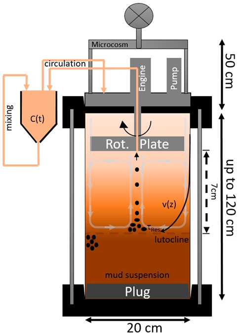
FIGURE 3. Sketch of the adapted Gems; sediments are eroded using a rotating plate to apply defined shear stresses at a specific depth; erodibility is derived from suspended sediment concentration concentration measurements.

Secondary flow patterns (gray arrows in Figure 3), which affect the uniform distribution of friction velocities on the sediment–water interface, are partly counteracted by a central suction. As a result, the applied shear stress is distributed nearly homogeneously (Gust, 1989; Gust und Müller, 1997). It is a feature of the Gems to apply controlled shear stresses on the sediment–water interface. In this way, the erodibility of sediments can be investigated assuring specific conditions, even though the stationary rotating flow might differ from the tidal flow. Water and eroded sediments are extracted in the center of the erosion chamber discharging water into the measurement chamber. SSC (C(t)) is determined by measuring turbidity between 0 g/L and 5 g/L every second using optical backscatter sensors developed at IWB and by measuring density between 1 g/L and 30 g/L every 5 min. Both devices are attached to the measurement chamber (upper left part of Figure 3). In contrast to previous studies using Gems, which discharge eroded sediments (Work und Schoellhamer, 2018), the sediment is kept in a closed erosion system to improve the representation of natural conditions (an increase of SSC above lutocline with increased tidal flow). Hence, the SSC increases during each experiment with every load step above critical shear stress. With the procedure used, net erosion is determined covering erosion and possible deposition occurring simultaneously. It is not yet possible to separate those two processes in the presented experimental procedure.

Erosion experiments are performed by placing the Gems on top of the sediment sample with a precalibrated distance of 7 cm between the stirring plate and the lutocline. Shear stress is increased in regular increments every 30 min. A defined shear stress is applied on the sediment surface by using a calibrated combination of stirrer revolutions per minute and the central suction flux following the relations

$u^{\ast }=-{2.0710}^{-5}{n}^2+{1.5710}^{-2}n+0.10527,(5)$

$Q=-0.0138n^2+5.5n+20,(6)$

where u* [cm/s] is the shear stress velocity, n [1/min] is the stirrer disc revolutions, and Q [ml/min] is the pump rate.

In case the applied shear exceeds the critical shear, during each load step interval, a repeating concentration pattern is expected to occur (see Figure 4). Before a change in concentration is recorded, a (small) lag time is expected because eroded sediments need to be transferred between the two chambers. This is followed by a relatively sharp increase in measured turbidity/density. Heading to the end of the load step, concentration gradients tend towards zero (respectively floc erosion rate in higher load steps). When erosion comes to an end, a new equilibrium is formed between the shear of flow and the erosion resistance of the sediment surface. In case the distance between the stirrer and sediment surface (primary lutocline) increases to more than 8 cm, the stirrer is readjusted to the default value of 7 cm to further obtain a defined shear stress. The evolution of the lutocline during erosion experiments results from taking close-up pictures in intervals of 1 min using a digital camera.

FIGURE 4

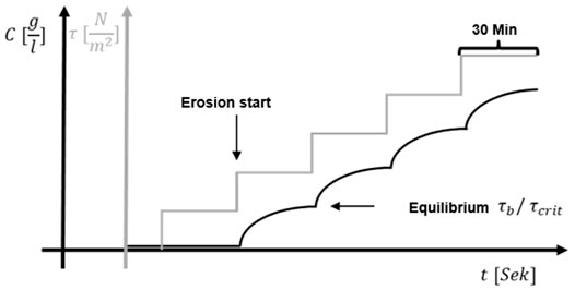
FIGURE 4. Methodology of load steps and suspended sediment concentration during an erosion experiment.

2.4.2 Processing of Turbidity Data

To observe the evolution of SSC over the experiment duration, a combination of turbidity and density measurements is needed to cover the range of concentrations occurring with an adequate technique. Sediment concentrations of up to 30 g/L have to be covered by both the turbidity and the density measurement. The turbidity measurements are run with a self-developed optical backscatter probe consisting of 10 optical sensors, while two sensors at a time cover the same concentration range. In this way, plausible SSC is measured in the range of 0 ≤ C ≤ 5 g/L using the backscatter probe. SSC above 5 g/l has to be covered by density measurements. The backscatter data is processed as follows:

- First, the turbidity value is calculated from measurement results (light value minus dark value) and smoothened by a moving mean filter of a window of 60 for the 10 sensors attached to the measurement probe.

- Second, the data of the different sensors are recalculated to SSC using a calibration curve generated specifically for Weser sediments.

- Third, by automatically combining data of the 10 sensors, a consistent concentration curve from the backscatter measurements is calculated.

2.4.3 Processing of Density Data

Density measurements carried out during an erosion experiment are processed as follows:

- SSC can be represented accurately by density measurements when SSC is above 0.5 – 1 g/L

- Process water density is measured at the beginning of the experiment where C << 1 g/L

- The densimeter also measures temperature, so measured densities are corrected for temperature changes during experiments

- Sediment concentration is calculated and an interpolated curve is formed to meet the same data frequency interval as the turbidity sensors.

As the last step, the two concentration curves are combined to form a representative time series of SSCs, covering the whole range of occurring SSCs during experiments.

Bulk density ρ_b of sediment suspensions can be expressed as the sum of the percentage (1—$\eta$) of the fluid (water) times its density ρ_w and the percentage of total suspended solids ($\eta$) times their dry density ρ_s:

${\rho }_b=\eta {\rho }_s+\left(1-\eta \right){\rho }_w={\rho }_w+\eta {\rho }_s-\eta {\rho }_w.(7)$

The volume percentage of sediment $\eta$ can be expressed as

$\eta =\frac{{\rho }_b-{\rho }_w}{{\rho }_s-{\rho }_w}.(8)$

By transformation of Eq. 7 and measures of bulk density, water density, and dry sediment density, the mass concentration of sediments C_Sed can be calculated:

$C_{sed}= \eta {\rho }_s={\rho }_b-{\rho }_w+\eta {\rho }_w.(9)$

In this study, bulk density ρ_b and water density ρ_w can be measured, while dry density ρ_s is estimated to be ρ_s = 2,575 kg/m³, measured by Malcherek (2010) as mean dry density for sediments of the investigated part of the Weser estuary. A best fit spline interpolation is used to extend density measurements to the frequency of the backscatter dataset. Both datasets are plotted together to finally combine the datasets. Derived concentration curves from both types of measurements are in good agreement within the interval 0.9 g/L≤ C ≤ 1.5 g/L. Depending on the quality of individual datasets, a point of that span is selected for each experiment to connect the datasets to a comprehensive time series of sediment concentrations. The connection point is set where residuals between the datasets become minimal.

In the next step, the time series of sediment concentration is used to derive erosion rates [kg/(m²/s)]. Here, each value of sediment concentration is related to the time increment between each data point and the average area of the sediment surface. Additionally, a 60 s moving average has been applied to reduce noise in the data. It must be noted that the calculated erosion flux represents the sum of deposition and erosion occurring at the same time. Hence, the derived parameter E_net is defined as net erosion:

$E_{net}=Erosion-Deposition.(10)$

3 Results

3.1 Sediment Characterization

As stated in Section 2.2, collected sediment samples from the Weser estuary have been characterized using classification tests for soil mechanics (grain sizes, WC, LOI). The mean results for the collected samples are summarized in Table 1 and described as follows. For both sites (BB and NH), the majority of grains (44–74%) are in silt size. Despite that, on average, the silt content is about 10% lower in samples from BB (54%) than in samples from NH (64%).

The clay to sand ratio ${\lambda }_{CS}$, the silt to clay ratio ${\lambda }_{SiC}$, and the ratio of fines to sand ${\lambda }_{SiCS}$ are used to predict the critical shear and cohesion of the mixture (Wu et al., 2018; van Rijn, 2020). For example, ${\lambda }_{CS}$ is above 1 for all samples from NH and below 1 for all samples from BB. As a consequence, the mean sand content in BB samples (28%) is significantly higher than that in NH samples (13%). The ratio of fines to sand ${\lambda }_{SiCS}$ is generally well below 10 and even below 4 for samples from BB. For NH samples, all values are above 4, including an outlier of sample NH-35, which is 23. For both sites, the critical amount of clay of 5–10% (Grabowski et al., 2011) is exceeded, so dominant cohesive behavior is expected (f_C(NH) ∼23%, f_C(BB) ∼18%). In general, the mean diameter is lower for samples from NH than BB because of a higher percentage of fines in NH samples. As more organic compounds can attach and survive at the (relatively) larger surface area of smaller particles, the experimental results exhibit a higher LOI in NH (12%) than in BB samples (9%). Depending on the (depth of the sub-) sample, WC shows high variability, ranging between 175% and 500% for NH samples and between 106% and 257% for BB samples. With regard to density, significantly higher values have been measured in the samples from BB. The samples from BB were mainly consolidated or in an advanced state of consolidation, sometimes having a layer of fresh deposits on top (MW-I). Samples from NH are rather in a viscous state, exhibiting densities around or slightly above gelling concentration.

An exemplary visual representation of the samples and differences between the sampling sites can be found in Figure 5 and Figure 6.

FIGURE 5

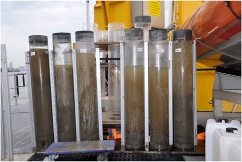
FIGURE 5. Sediment samples taken from Weser-km 63, Blexer Bogen, on 26.07.2021.

FIGURE 6

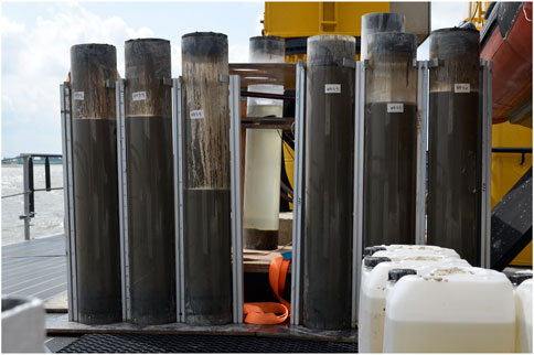
FIGURE 6. Sediment samples taken from Weser-km 56, Nordenham, on 28.07.2021.

In addition to Table 1, Figure 7 shows the percentage breakdown of grain sizes and the corresponding classification using the U.S. Department of Agriculture’s (USDA) textural triangle for evaluated (sub-) samples from BB (blue) at Weser-km 63 and NH (white) at Weser-km 56. While most samples are in the range of silt loam, similarities and differences between the sample sites become apparent. Both samples have very similar silt content, so the clay to sand ratio represents differences in the sediment composition fairly well.

FIGURE 7

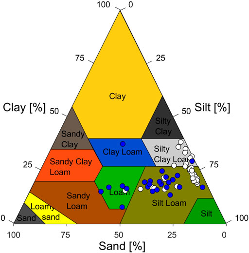
FIGURE 7. U.S. Department of Agriculture’s Classification (United States Department of Agriculture, 1987) of sediments taken from the Weser estuary at the site of Nordenham, Weser-km 56 (white dots), and Blexer Bogen, Weser-km 63 (blue dots).

3.2 Density

Density profiles of sediment cores kept in natural stratification have been determined for sediments taken during field campaigns (MW-I, MW-II, MW-III). Figure 8 shows the results of the profiles of 4 samples from BB and 9 samples from NH. Densities are related to the observed sediment–water interface (zero level) in the sediment cores as the lutocline is seen as the reference standard for comparison of the samples when it comes to density. Profiles for sediments from BB (left plot) exhibit densities in the range of 1,000–1,400 kg/m³, showing a steep gradient or even starting as high as 1,200 kg/m³ in density. During MW-I, a mobile mud layer of ∼10–25 cm in height is observed in both samples (BB-04 and BB-05) on top of a layer of higher density exhibiting a secondary lutocline to (pre-) consolidated sediment. In sediment cores taken during MW-III, no mobile mud layer is observed and the profile starts at densities of 1,200 kg/m³, leading to values of 1,300 kg/m³ in the lower part of the cores. Closer to the center of the ETM, here located in NH, we observe a lower density range between 1,050 and 1,300 kg/m³ in all cores. Fresh mobile and stationary mud suspension in the range of 1,050–1,150 kg/m³ is seen in all sediment samples taken from NH. It is worth mentioning that during campaign MW-II, a more dense (pre-) consolidated stage of sediment suspension is observed in the lower half of the samples (NH-13, NH-14, and NH-16).

FIGURE 8

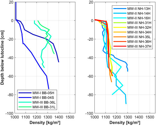
FIGURE 8. Density profiles below lutocline of sediment samples collected in three campaigns (MW-I, MW-II, MW-III) at locations in Blexer Bogen (BB, left) and Nordenham (NH, right); measurement location in L (lab), H (harbor), or S (ship).

The observations lead to the conclusion that the sedimentation foci are also reflected in the density profiles. Samples from BB exhibit sediments mostly in the preconsolidated and consolidated stage, following a classification stated by Kombiadou and Krestenitis (2013), while sediments taken from NH are classified as (mobile and stationary) mud.

Results of the consolidation experiments conducted with remolded samples in the laboratory are depicted in Figure 9, showing the density evolution and the lutocline evolution over a period of 24 h. Two major phases of settling can be observed. Samples with initial densities below the structural density reveal hindered settling behavior at the beginning of the experiment, reaching maximum settling velocities of w_s ∼ 0,4 mm/s. When the lutocline descends at settling velocity in the hindered settling regime, densities in the upper column decrease sharply, while densities below the lutocline increase because of reduced space for the same amount of solids. After a few hours (∼4 h for 1,065 kg/m³ suspensions, ∼9 h for 1,080 kg/m³ suspensions), the settling velocity reduces significantly, the suspensions reach the point of concentration (Winterwerp et al., 2021), consolidation starts in the permeability phase (van Rijn, 2020), and rates of consolidation become as small as w_c = 2*10^–3–2*10^–2 mm/s.

FIGURE 9

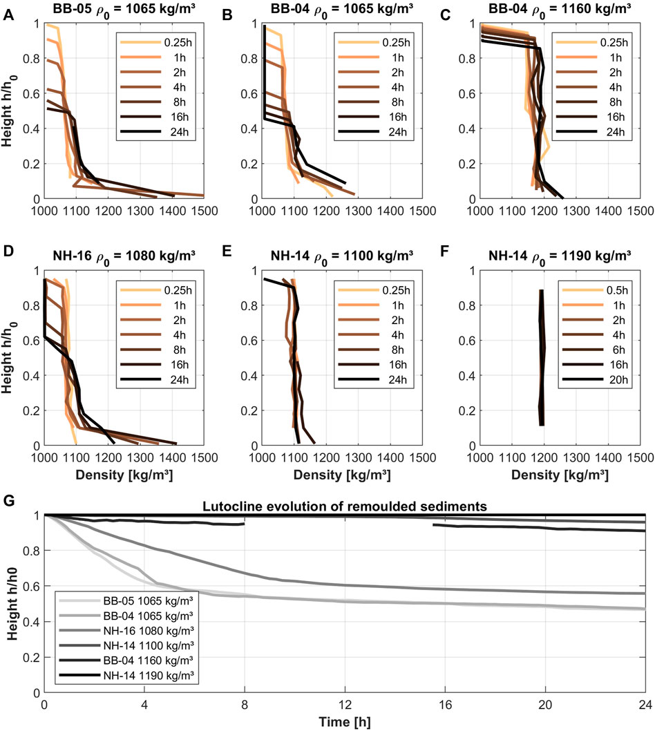
FIGURE 9. Evolution of primary lutocline (G) of remolded natural sediments from Blexer Bogen and Nordenham and corresponding evolution of density profiles: sample code (sc) BB-05 and initial density ρ₀ = 1,065 kg/m³ (A), sc: BB-04 and ρ₀ = 1,065 kg/m³ (B), sc: BB-04 and ρ₀ = 1,160 kg/m³ (C), sc: NH-16 and ρ₀ = 1,080 kg/m³ (D), sc: NH-14 and ρ₀ = 1,100 kg/m³ (E), and sc: NH-14 and ρ₀ = 1,190 kg/m³ (F); h₀ = h(t=0), h = h(t=t_i).

While compaction proceeds, the density increases sharply at the bottom of the sample and slightly in the rest of the column. For samples with initial densities above the structural density, no hindered settling regime is observed. The suspensions are stable over the observation period of 24 h. Because a major shift in the settling behavior could be observed between initial densities of ρ₀ = 1,080 kg/m³ and ρ₀ = 1,100 kg/m³, structural density ρ_gel (or gelling concentration C_gel) is expected to be in the median range. Because of a higher clay content in NH and a higher sand content in BB samples, it is expected that the structural density for samples from NH is slightly lower (approx. ρ₀ = 1,085 kg/m³) than the structural density for samples from BB (approx. ρ₀ = 1,100 kg/m³). Applying Eq. 9 using a water density of ρ_w = 1,009 kg/m³ and a dry sediment density of ρ_s = 2,575 kg/m³, the corresponding gelling concentration for NH is C_gel,NH = 125 g/L and for BB is C_gel,BB = 150 g/L.

3.3 Erosion

3.3.1 Quasi In Situ Erodibility

The erodibility of nearly undisturbed natural sediment samples has been investigated quasi in situ using a Gems erosion chamber. Sediments have been extracted and transported carefully to the harbor, where the first experiments took place straight after sampling. Two samples each have been investigated from BB and NH during campaign MW-III. Measured sediment concentrations and derived erosion rates are presented in Figure 10. The experiment duration was primarily dependent on the general conditions during the field trips and the sediment responses during the experiments. The same methodology was applied in all experiments, and at least six load steps up to τ_b = 0.12 N/m² have been applied to every sample, although in some experiments, higher shear stresses could be applied.

FIGURE 10

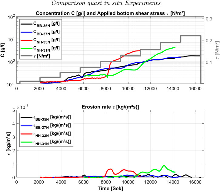
FIGURE 10. Sediment concentration and derived erosion rate for sediment samples collected from the Weser estuary without any further handling.

For all samples, the applied shear stresses lead to an increase in SSC in the measurement chamber of the Gems; hence, it is assumed that erosion took place. It should be noted that experiments on sample BB-37 and sample NH-33 were carried out approx. 24 h after extraction because experiments for the other samples were carried out first. It should also be stated that backscatter data at the beginning of the experiments were very noisy for no apparent reason, so some data needed to be excluded from the analysis. Sample BB-35, BB-37, and NH-33 data from the first load step and sample NH-31 data from the first three load steps had to be excluded from the analysis.

For experiments using samples from BB, the concentration evolution is very similar. The onset of erosion is observed to be in load step 3 with τ_b = 0.05 Pa. In the following steps, concentration seems to increase continuously, but following the pattern of theoretical behavior drawn in Figure 4. In load step eight, both experiments using BB samples show concentrations of approx. C ∼ 1.5 g/L. Derived maximum erosion rates are well below ε < 10^–3 [kg/(m²s)]. Hence, they do not pass critical rates for mass erosion. This confirms the visual observations during the experiments and is consistent with high densities (thus, high erosion resistance) measured in the other samples from BB during campaign MW-III. Compared to results from experiments using NH samples, the differences are obvious here. Homogeneous density profiles (Figure 8) with significantly lower densities closely above the gelling point suggest higher erodibility. This assumption is confirmed by the experiments because at shear stresses of τ_b = 0.1–0.12 N/m², the NH samples exhibit a sudden increase in the sediment concentration and erosion rates reach ε = 0.5 × 10^–3 kg/(m²s), which is set as the threshold for mass erosion derived in laboratory experiments, presented in Section 3.3.3. SSC increases sharply, reaching values of approx. 3 g/L at the end of the experiments. The determined critical shear for floc erosion is τ_cr,Ef ∼ 0.05–0.07 N/m² with floc erosion rates of approx. ε_f = 5 × 10^–5 [kg/(m²s)].

3.3.2 Erodibility in Single Experiments

Exemplary results of experiments and comparisons of those with initial densities of ρ₀ ∼ 1,065 kg/m³ and ρ₀ ∼ 1,125 kg/m³ with corresponding consolidation times of 3 h and 18/24 h are shown in Figures 11A–D. For the experiments with suspension densities below the structural density, the initiation of erosion is observed in load steps three to four, which corresponds to a critical shear stress for floc erosion of τ_cr,Ef = 0.05–0.07 N/m² and erosion rates of ε_f = 10^–4 [kg/(m²s)]. Mass erosion is observed to start at load stage four, corresponding to τ_cr,Em = 0.07 N/m², when the consolidation time is 3 h or below. Mass erosion rates reach up to ε_m = 5 × 10^–3 [kg/(m²s)] in this case. On the other hand, the increase in erosion resistance of sediment suspensions below the gelling point runs fast. After a consolidation time of 18 h, mass erosion starts first in load stage eight, corresponding to a critical shear stress of τ_cr,Em = 0.18 N/m², exhibiting similar erosion rates of ε_m = 5 × 10^–3 [kg/(m²s)] as in load step four. If the gelling concentration is expected to be developed after 4–10 h (depending on initial density), this confirms the assumption made before that the increase in erosion resistance slows down significantly after reaching the gelling state. As proof, sediment suspensions investigated with initial densities above the gelling point exhibit similar behavior. Floc erosion is seen repeatedly after surpassing load step four, while mass erosion occurs when load step nine is reached, corresponding to a critical shear stress of τ_cr,Em = 0,21 N/m² and erosion rates of ε_m = 5 × 10^–3 kg/(m²/s). Transferred to natural conditions, this means that if a fresh mud deposit withstands the tidal flow for a few hours or even increases in sediment concentration by deposits during slack tide, it becomes immobile and relatively stable against erosive forces (compared to deposits below the gelling point). With the results presented here, we assume confirmation of repeatability of experiments under the same experimental conditions (leaving an individual variability).

FIGURE 11

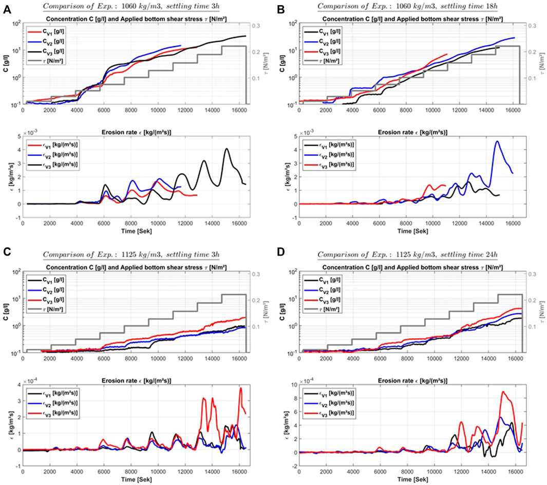
FIGURE 11. Steps of applied bottom shear and concentration (upper) and erosion rate evolution (lower) in single experiments: Comparison of results with densities of ρ₀ = 1,060 kg/m³ and consolidation times of 3 h (A), ρ₀ = 1,060 kg/m³ and consolidation times of 18 h (B), ρ₀ = 1,125 kg/m³ and consolidation times of 3 h (C), and ρ₀ = 1,125 kg/m³ and consolidation times of 24 h (D).

3.3.3 Erosion and Resuspension Characteristics

Erodibility. In this section, an overview of the results from experiments conducted in the laboratory and the field is presented. As shown in Section 3.3.2, with respect to variability, especially under mass erosion conditions, repeatable behavior could be established between experiments run under the same conditions. To highlight dependencies, it makes sense to consider the results of a set of experiments. If the eroded mass at the end of each load step is measured and plotted against the applied shear stress on a double logarithmic plot, the logarithmic relationship between the shear stress and erosion rate becomes visible. The overall behavior of investigated sediments is presented in Figure 12. In the case of remolded samples having initial densities below the gelling point, an increase in erosion resistance is observed within 24 h, corresponding with decreased erosion rates (respectively eroded mass) and increased critical shear. When the initial density of the remolded samples exceeds the gelling point, a general change in the erodibility is observed. In this stage, lasting for at least 24 h, eroded mass per applied shear stress does not primarily depend on time anymore, and erodibility varies within a range of one logarithmic degree. Other influencing parameters become dominant as settling velocities reduce to speed of consolidation and almost all interparticle bonds have been established. Moreover, it has to be emphasized that the slope of the erodibility is very similar in all laboratory-based erosion experiments. For comparison, the results from the quasi in situ experiments are also highlighted in Figure 12 as dotted lines. While the variability between the load steps appears to be slightly higher than that in the laboratory experiments, all results from the quasi in situ experiments lie in the range of the laboratory-investigated sediment samples. Actually, all of the lines resulting from the quasi in situ experiments are in the transition zone between fresh deposits of mobile mud below the gelling point and stationary mud above the gelling point.

FIGURE 12

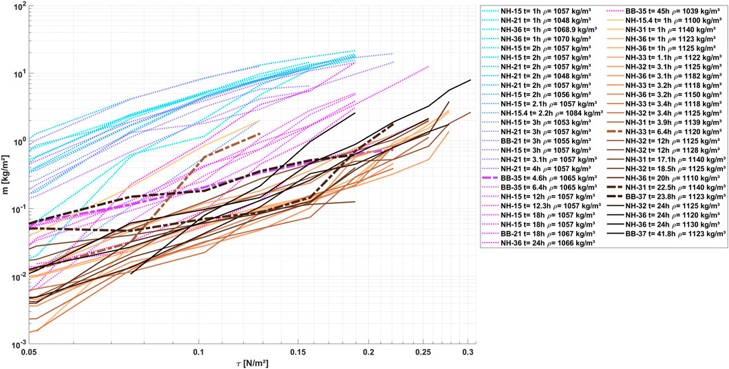
FIGURE 12. Results of experiments undertaken, displaying the eroded mass [kg/m²] vs. applied shear stresses [N/m²]; experiments with initial densities below (dotted lines) and above (solid lines) are shown, while initial settling times are distinct with using two colormaps (bluish and brownish). Results from the quasi in situ experiments are displayed as big dashed lines.

Erosion modes. Three modes of erosion have been observed in this study:

- Particle or floc erosion: In every single experiment, erosion started with a small increase in sediment concentration already at very low shear stresses. No immediate change in lutocline height (dh < 1 mm) can be observed, and only single particles or flocs get into the water column, changing SSC by only C < 0.1 g/L. Erosion depth is below a millimeter range during a load step, and the turbidity of the water column increases slightly.

- Surface erosion: During some experiments, the second stage of erosion was observed, when plates of connected flocs or several layers of flocs were eroded, building craters and grooves along the flow direction. Sediment concentration in the water column increases slowly by C ∼ 0.1–0.2 g/L, and erosion depth reaches one to a few millimeters within each load step (on some parts of the sediment–water surface).

- Mass erosion: The sediment surface breaks up because the applied shear stress is larger than the undrained (remolded) soil strength of the bed (van Rijn, 2020), and huge chunks of sediment are eroded within a short amount of time. Erosion depth increases fast while reaching a depth of a few centimeters, and sediment concentration in the water column rises by several grams per liter during a load step.

Because the transition between floc and surface erosion appears to be fluent and the distinction from measured erosion data is challenging, we do not differ between those two erosion modes in this study. Specific surface erosion was only visible in personal observations during the experiments.

Following the procedure described in Section 2.4, parameter values for the critical shear for floc erosion, the floc erosion rate, and the critical shear for mass erosion have been derived for all the experiments. Results for parameters related to floc erosion are presented in Figure 13.

FIGURE 13

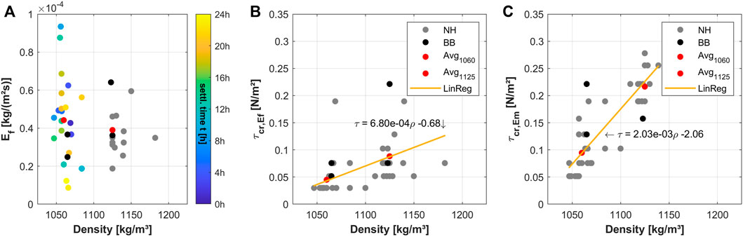
FIGURE 13. Derived erosion rate for floc erosion ε_f (A) and corresponding critical shear stress τ_cr,Ef for floc erosion (B) as well as critical shear stress for mass erosion τ_cr,Em (C); regression lines are fitted based on gray data points.

In all plots of Figure 13, gray dots depict samples from NH, black dots depict samples from BB, and red dots represent the mean values of erosion parameters for low and high initial densities. Regression lines are based on the scattering of measured points. Left hand (A), the mean of the maximum erosion rate of every shear stress step within the floc erosion range is given. Dot colors indicate the settling time of suspensions with initial densities below the gelling point (∼1,060 kg/m³). It becomes clear that the settling time for sediments from the Weser estuary does not play a significant role in the determination of floc erosion rates, although the variability of erosion rates reduces when investigating suspensions above the gelling point. Both averages of erosion rates for high and low initial densities are about ε_f = 4 × 10^–5 [kg/(m²s)]. Figure 13B relates detected critical shear stresses for floc erosion to initial suspension densities. Corresponding critical shear for floc erosion is about τ_cr,Ef = 0.05 N/m² for low and about τ_cr,Ef = 0.09 N/m² for high initial densities. To distinguish between the results from NH and BB in detail, more samples from BB have to be analyzed. Besides, measured values for critical shear seem to be higher for BB samples (as expected because of a higher sand content). Regarding critical shear for mass erosion, differences between the suspension erodibility become even more clear, with τ_cr,Em = 0.09 N/m² for the low- and τ_cr,Em = 0.21 N/m² for the high-density range.

Derived parameter values for floc and mass erosion are summarized in Table 2. While laboratory-remolded sediment samples exhibit a dependency of erosion parameters for floc erosion on density rather than settling time, critical shear for mass erosion already increases within the hindered settling regime (first 24 h after low initial density deposit). Investigated natural experiments from NH show similar behavior in terms of floc erosion. For mass erosion, natural behavior is best represented by samples of low initial density and settling times of 6–24 h (meaning self-developed gelling point). This might be due to segregation happening in the field and in the laboratory when starting with lower initial densities of suspensions. When a suspension is remolded with densities above the gelling point, segregation of sand particles might be prohibited. Floc erosion patterns are similar in natural sediments (with high densities) from BB, but critical shear for mass erosion was not exceeded in experiments with applied shear of up to 0.21 N/m². This underlines the expected degree of consolidation for samples from BB and highlights further required experiments on natural specimens with even higher densities.

TABLE 2

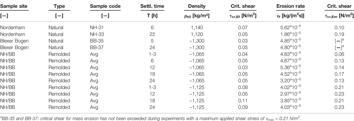
TABLE 2. Results of experiments with natural sediment samples and remolded sediment samples of two density ranges and four different settling times: critical shear stress and erosion rates determined for floc erosion and mass erosion.

When using the derived parameters (ε_f, τ_cr,Ef, τ_cr,Em) for a first fit of the erosion models introduced in Section 1, one can see that it is possible to represent a part of the variability in erodibility observed in the presented experimental results. Applying an erosion constant of E_0,mud = 10^–4 kg/(m²s) and a critical shear of τ_cr = 0.05 N/m², the Partheniades model can represent the erodibility of samples above the gelling point, lying in the lower spectrum of Figure 12. The model by Sanford and Maa is applied using parameter values of β = 5 × 10^–5 (m²s)/kg and the same critical shear as in the Partheniades model. The resulting erosion rates of this model are in the upper part of the spectrum presented in Figure 12.

4 Discussion and Conclusion

4.1 Summary and Discussion

In this study, results from quasi in situ and laboratory-based experiments investigating aspects of the bed exchange behavior are reported and discussed. Sediment characteristics, shortly after deposition, being in a soft state but accounting for long-term deposition, is the subject of this investigation. For this purpose, natural sediments from the center of the navigational channel within the ETM of the Weser estuary at sites in BB (more downstream) and NH (more upstream) are collected. Taken during slack water with a novel sediment sampler, sediment cores cover the transition between the lower water column and the upper sediment bed. The sediment sampler and the experimental setup have been coordinated during development. This allowed sediment samples to be placed directly into the experimental setup for tests of erodibility after collection. Representative remolded samples in terms of density and composition have been investigated later in the laboratory. Results from erosion experiments with naturally stratified sediments are used to estimate the magnitude of quasi in situ erodibility, while results from laboratory-remolded natural sediments are used to investigate the variability under defined laboratory conditions. The settling and consolidation behavior have been investigated by deriving density profiles and lutocline evolution from naturally stratified sediments and laboratory-remolded sediments with varying initial densities. In addition, sediments are classified by deriving grain size percentage breakdown, WC, and LOI.

The condition of the samples taken confirm the existence of a fluffy mud layer covering a comparatively solid bed, if the ETM is present at the specific location. The layer thickness of the fluffy layer was observed to be in the range of a few decimeters up to 1 m and slightly above. Classification experiments prove the existence of clay, silt, and sand, all of which are in significant proportions. According to the USDA code, collected Weser sediments are mainly classified as silt loam. Sediments from BB contain about 10% more sand and lesser mud to the same extent compared to sediments from NH. Higher and increasing densities with depth up to values of ρ_b ∼ 1,400 kg/m³ are observed for samples from BB. Samples from NH exhibit more homogeneous densities and sedimentological profiles. Densities of NH samples are in the range of ρ_b ∼ 1,050–1,250 kg/m³, sometimes from top to bottom exhibiting densities of about ρ_b ∼ 1,125 kg/m³. The quasi in situ measurements confirm the existence of both mobile and stationary mud layers within the ETM at the time of sampling. Also, this confirms the absence of large fluid mud layers at the lateral ETM boundaries, meaning BB in this case. Investigations of the density evolution in the laboratory prove the cohesive behavior of the mixture. Settling is hindered for experiments with remolded CBS below structural density. From the density profiles and lutocline evolution, a gelling concentration could be determined at approx. C_gel = 125–150 g/L respective ρ_gel = 1,085–1,100 kg/m³. After exceeding the gelling concentration, settling velocities of about w_s = 0,4 mm/s reduce significantly. Then, consolidation is expected to start (in the permeability phase first, then effective stresses become dominant), exhibiting significantly lower velocities of w_c = 2 × 10^–3–2 × 10^–2 mm/s.

Erodibility is investigated by analyzing the evolution of sediment concentration above the lutocline and resulting erosion rates. Critical shear for floc and mass erosion is derived from collected data. In the laboratory, remolded samples with defined initial conditions are used. Remolded samples either exhibit initial bulk densities of approx. ρ = 1,065 kg/m³ below structural density or they exhibit densities of approx. ρ = 1,125 kg/m³ above structural density. While erodibility decreases during the first 24 h in the preconsolidation phase, no such decrease is observed to happen in the same interval for suspensions with initial densities above the gelling point. Increased erosion resistance results in higher critical shear stresses and lower erosion rates. Critical shear stress for floc erosion have been observed to be below 0.1 N/m² for both natural and remolded samples, leading to erosion rates of about 4 × 10^–5 kg/(m²s) for all experiments. When sediments are freshly deposited from the water column, densities of 1,050–1,070 kg/m³ are observed, exhibiting very low critical shear values for mass erosion of about 0.06 N/m², similar to the fact that the sediments are settling quite fast in this phase, the erodibility decreases and critical shear for mass erosion increases to values of 0.17 N/m². Regarding suspensions with initial densities above the gelling point, no consistent change could be observed for all the parameters investigated within a period of 24 h. Density profiles remain homogeneous, and erodibility parameters remain approx. constant with critical shear for mass erosion in the range of 0.21–0.23 N/m². The best representation of investigated natural erodibility is observed to occur when sediments in suspensions below structural density settle for about 6–10 h. Here, initial density is increased to reach the point of concentration, but critical shear for mass erosion stays below that found for suspensions created above structural density, likely because of segregation processes happening in the hindered settling phase. It is also found that the erodibility of investigated sediment suspensions above the gelling point can be represented using the Partheniades approach, while soft mud suspensions below the gelling point are better represented using the approach by Sanford and Maa.

4.2 Conclusion

The challenge of understanding the processes leading to net sedimentation and accumulation of cohesive sediments in the Weser estuary in reach of the ETM is addressed in this study. Methods and experimental facilities have been developed to investigate the bed exchange behavior of freshly deposited natural sediments in quasi in situ and laboratory experiments. Generated density profiles of collected, mostly undisturbed cores confirm the existence of mobile and stationary mud layers on top of a relatively dense bed. Mobile (below) and stationary (above) mud exhibit densities in the reach of the gelling point. Investigations on erodibility have shown that mobile suspensions below the gelling point settle quite fast while increasing erosion resistance at the same time. Instead, stationary suspensions above the gelling point do not settle or significantly increase erosion resistance in the considered period of 24 h after layer generation. Ultimately, the results discussed support the hypothesis formulated in Introduction on how cohesive sediments may accumulate in the navigational channel of an estuary. Within the turbidity zone of the Weser estuary, cohesive sediments may form a layer with concentrations exceeding gelling concentration. Extected to partly withstand a tidal cycle, the layer dampens the erosive forces of the tidal current and thus favors long-term consolidation processes in the lower part of the layer.

4.3 Limitations

The developed methods work well in the expected ranges they cover. While we are convinced to have covered the upper sediment layers with minor disturbance, it has to be proven in further campaigns that density profiles measured using the developed methodology are comparable to densities derived by other in situ techniques. The first comparison to low-resolution data from MBES indicates a good agreement, but further evidence is needed. The results derived from the erosion experiments are in the range of the results obtained by other studies published recently. Nevertheless, it is necessary to mention that deriving a consistent time series for SSC and erosion rates is a huge endeavor because two different measurement techniques are used. Future optimizations of the experimental facility should consider sensors covering the whole range of observed SSCs during experiments.

4.4 Outlook

As the next steps of this investigation, it is planned to fit and evaluate erosion models based on the presented dataset. Density profiles and lutocline evolution are used to derive parameters from the Gibson model by applying the approach from Merckelbach and Kranenburg (2004). In addition, in further investigations of sediment erodibility, a dynamic forcing with sinusoidal bidirectional flow comparable to tidal flow should be undertaken. The enhanced Gems presented in this study are capable of introducing such dynamic forcing so these investigations are considered to be a consistent next step. Moreover, a further set of experiments is in progress where the erodibility is related to sediments with densities in the range of consolidated beds. The aim is to derive a single approach capable of representing the variability in erodibility of fresh sediment deposits from the Weser estuary observed in nature and the laboratory.

Data Availability Statement

The raw data supporting the conclusion of this article can be provided upon request at the corresponding authors contact.

Author Contributions

JP designed and performed the experiments, analyzed the data, and wrote the manuscript; PF and EN helped with the design of the experiments, data interpretation, and writing of the manuscript; RH assisted with data interpretation and writing of the manuscript.

Funding

Being part of the research project FAUST (for an improved understanding of estuarine sediment transport), this study was supported with funding from the Federal Waterways Engineering and Research Institute Germany (BAW) and with support from the (WSA) by providing ship capacities and employees. Publishing fees are funded by the Deutsche Forschungsgemeinschaft (DFG, German Research Foundation)—Projektnummer 491268466—and the Hamburg University of Technology (TUHH) in the funding program *Open Access Publishing*.

Conflict of Interest

The authors declare that the research was conducted in the absence of any commercial or financial relationships that could be construed as a potential conflict of interest.

Publisher’s Note

All claims expressed in this article are solely those of the authors and do not necessarily represent those of their affiliated organizations, or those of the publisher, the editors and the reviewers. Any product that may be evaluated in this article, or claim that may be made by its manufacturer, is not guaranteed or endorsed by the publisher.

Acknowledgments

The authors would like to deeply thank all the people involved in conducting the field trips and laboratory experiments. In addition, we’d like to thank the BAW for funding the research and the waterways and shipping administration in Bremerhaven for help in conducting field trips by providing capacity of ships and employees.

References

Becker, M., Maushake, C., and Winter, C. (2018). Observations of Mud‐Induced Periodic Stratification in a Hyperturbid Estuary. Geophys. Res. Lett. 45 (11), 5461–5469. doi:10.1029/2018GL077966

CrossRef Full Text | Google Scholar

Chen, D., Zheng, J., Zhang, C., Guan, D., Li, Y., and Wang, Y. (2021). Critical Shear Stress for Erosion of Sand-Mud Mixtures and Pure Mud. Front. Mar. Sci. 8, 3039. doi:10.3389/fmars.2021.713039

CrossRef Full Text | Google Scholar

Eberle, M., Fiedler, M., Blasi, C., König, F., Schöl, A., Schubert, B., et al. (2014). Sedimentmanagementkonzept Tideweser-Bericht. Untersuchung im Auftrag der WSÄ Bremen und Bremerhaven. Bundesanstalt für Gewässerkunde (BfG). Koblenz: BfG-Bericht 1794.

Google Scholar

Gounder Krishnappan, B., Stone, M., Granger, S., Upadhayay, H., Tang, Q., Zhang, Y., et al. (2020). Experimental Investigation of Erosion Characteristics of Fine-Grained Cohesive Sediments. Water 12 (5), 1511. doi:10.3390/w12051511

CrossRef Full Text | Google Scholar

Grabemann, I. (1992). Die Trübungszone im Weser-Ästuar: Messungen und Interpretation. Dissertation. Universität Hamburg, Geesthacht. Geesthacht: GKSS Forschungszentrum.

Google Scholar

Grabowski, R. C., Droppo, I. G., and Wharton, G. (2011). Erodibility of Cohesive Sediment: The Importance of Sediment Properties. Earth-Science Rev. 105 (3-4), 101–120. doi:10.1016/j.earscirev.2011.01.008

CrossRef Full Text | Google Scholar

Gust, G. (1989). Method of Generating Precisely-Defined Wall Shearing stresses11.10.1989. St. Petersburg, Florida: Applicant Hydro Data Inc.,. Application number: 419649. Patent number: US4973165.

Google Scholar

Gust, G., and Müller, V. (1997). “Interfacial Hydrodynamics and Entrainment Functions of Currently Used Erosion Devices,” in Cohesive Sediments, 149174.

Google Scholar

Hesse, R. (2020). Zur Modellierung des Transports kohäsiver Sedimente am Beispiel des Weserästuars. dissertation. Hamburg: Technische Universität Hamburg, Institut für Wasserbau.

Google Scholar

Kombiadou, K., and Krestenitis, N. (2013). “Modelling Cohesive Sediment Dynamics in the Marine Environment,” in Sediment Transport Processes and Their Modelling Applications. Croatia. Editor M. H. G. Andrew James (InTech). doi:10.5772/51061

CrossRef Full Text | Google Scholar

Kösters, F., Grabemann, I., and Schubert, R. (2018). “Die Schwebstoffdynamik in der Trübungszone des Weserästuars. Kuratorium für Forschung im Küsteningenieurwesen,” in Die Küste (86). zuletzt geprüft am 08.01.2020.

Google Scholar

Kranenburg, C., and Winterwerp, J. C. (1997). Erosion of Fluid Mud Layers. I: Entrainment Model. J. Hydraulic Eng. 123123 (6504), 5046–5511. doi:10.1061/(asce)0733-9429(1997)123:6(504)

CrossRef Full Text | Google Scholar

Krishnappan, B. G. (2000). “Modelling Cohesive Sediment Transport in Rivers. The Role of Erosion and Sediment Transport in Nutrient and Contaminent Transfer (Proceedings),” in IAHS Publikationen, 269–276. zuletzt geprüft am 11.03.2022.

Google Scholar

Lange, D., Müller, H., Piechotta, F., and Schubert, R. (2008). “The Weser Estuary,” in Die Küste. S. 275–287Online verfügbar unter Available at: https://hdl.handle.net/20.500.11970/101611, zuletzt geprüft am 04.01.2022.

Google Scholar

Malcherek, A. (2010): Zur Beschreibung der rheologischen Eigenschaften von Flüssigschlicken. Die Küste (77)135–178.

Google Scholar

Mengual, B., Hir, P., Cayocca, F., Garlan, T., and Garlan, T. (2017). Modelling Fine Sediment Dynamics: Towards a Common Erosion Law for Fine Sand, Mud and Mixtures. Water 9 (8), 564. doi:10.3390/w9080564

CrossRef Full Text | Google Scholar

Merckelbach, L. M., and Kranenburg, C. (2004). Determining Effective Stress and Permeability Equations for Soft Mud from Simple Laboratory Experiments. Géotechnique 54 (9), 581–591. doi:10.1680/geot.2004.54.9.581

CrossRef Full Text | Google Scholar

Papenmeier, S., Schrottke, K., Bartholomä, A., and Flemming, B. W. (2013). Sedimentological and Rheological Properties of the Water-Solid Bed Interface in the Weser and Ems Estuaries, North Sea, Germany: Implications for Fluid Mud Classification. J. Coast. Res. 289, 797–808. doi:10.2112/JCOASTRES-D-11-00144.1

CrossRef Full Text | Google Scholar

Parchure, T. M., and Mehta, A. J. (1985). Erosion of Soft Cohesive Sediment Deposits. J. Hydraulic Eng. 111111 (10), 130810–131326. doi:10.1061/(ASCE)0733-942910.1061/(asce)0733-9429(1985)111:10(1308)

CrossRef Full Text | Google Scholar

Partheniades, E. (1965). Erosion and Deposition of Cohesive Soils. J. Hydraulic Div HY1 (91), 105–139. doi:10.1061/jyceaj.0001165

CrossRef Full Text | Google Scholar

Patzke, J., Hesse, R., Zorndt, A., Nehlsen, E., and Fröhle, P. (2019). Conceptual design for investigations on natural cohesive sediments from the Weser estuary. Hg. v. INTERCOH 2019. TU Hamburg. Istanbul.: Institut für Wasserbau. Online verfügbar unter. doi:10.15480/882.3599

CrossRef Full Text | Google Scholar

Sanford, L. P., and Maa, J. P.-Y. (2001). A Unified Erosion Formulation for Fine Sediments. Mar. Geol. 179 (1-2), 9–23. doi:10.1016/S0025-3227(01)00201-8

CrossRef Full Text | Google Scholar

Schweim, C. (2005). Modellierung und Prognose der Erosion feiner Sedimente. Dissertation. RWTH, Aachen: Bauingenieurwesen.

Google Scholar

Shields, A. (1936). Anwendung der Ähnlichkeitsmechanik und der Turbulenzforschung auf die Geschiebebewegung. Berlin: Technische Hochschule BerlinPreußische Versuchsanstalt für Wasserbau.

Google Scholar

Torfs, H., Mitchener, H. J., Huysentruyt, H., and Toorman, E. A. (1996). Settling and Consolidation of Mud/sand Mixtures. Coast. Eng. 2927 (1-2)–45. doi:10.1016/S0378-3839(96)00013-0

CrossRef Full Text | Google Scholar

United States Department of Agriculture (1987). Soil Mechanics Level 1-Module 3. USDA Textural Classification-Study Guide. Washington, D. C: Soil Conservation Service.

Google Scholar

Van Rijn, L. C. (2020). Erodibility of Mud–Sand Bed Mixtures. J. Hydraul. Eng. 146 (1), 4019050. doi:10.1061/(ASCE)HY.1943-7900.0001677

CrossRef Full Text | Google Scholar

Van Rijn, L. C. (2016). Fluid Mud Formation. Online verfügbar unterzuletzt geprüftAvailable at: www.leovanrijn-sediment.com.

Google Scholar

Van Rijn, L. C. (1993). Principles of Sediment Transport in Rivers, Estuaries and Coastal Seas. 1 Band. Utrecht: Aqua Publications, zuletzt geprüft am 03.09.2018.

Google Scholar

Whitehouse, R. J. S., Soulsby, R. L., Spearman, J., Roberts, W., and Mitchener, H. J. (2000). Dynamics of Estuarine Muds. A Manual for Practical Applications. London: Telford.

Google Scholar

William, H., McAnally und Ashish, J., and Mehta, Hg. (2000). “Coastal and Estuarine Fine Sediment Processes, Bd. 1st Edn, 3 (Amsterdam: Elsevier Science), v–viii. doi:10.1016/s1568-2692(00)80107-2

CrossRef Full Text | Google Scholar

Winterwerp, J. C., Christian, J., van Kessel, T., Dirk, S., van Prooijen, , et al. (2021). Fine Sediment in Open Water. 55. World Scientific.

Google Scholar

Winterwerp, J. C., and van Kesteren, W. G. M. (2004). “9 - Erosion and Entrainment,” in Johan Christian Winterwerp und Walther van Kesteren (Hg.): Introduction to the Physics of Cohesive Sediment in the Marine Environment. Bd. 56: Elsevier (Developments in Sedimentology), S. 343–381. Online verfügbar unter Available at: http://www.sciencedirect.com/science/article/pii/S0070457104800104.

Google Scholar

Work, Paul. A., and Schoellhamer, D. H. (2018). Measurements of Erosion Potential Using Gust Chamber in Yolo Bypass Near Sacramento, California. Reston, Virginia: Hg. v. US Geological Survey, US Department of the Interior und California Department of Water Resources. US Geological Survey. zuletzt geprüft am 22.08.2019.

Google Scholar

Wu, W., Perera, C., Smith, J., and Sanchez, A. (2018). Critical Shear Stress for Erosion of Sand and Mud Mixtures. J. Hydraulic Res. 56 (1), 96–110. doi:10.1080/00221686.2017.1300195

CrossRef Full Text | Google Scholar