
94% of researchers rate our articles as excellent or good
Learn more about the work of our research integrity team to safeguard the quality of each article we publish.
Find out more
ORIGINAL RESEARCH article
Front. Earth Sci., 22 July 2022
Sec. Interdisciplinary Climate Studies
Volume 10 - 2022 | https://doi.org/10.3389/feart.2022.912048
This article is part of the Research TopicVegetation Phenology and Response to Climate ChangeView all 8 articles
 Idaline Laigle1*
 Bradley Z. Carlson1
 Anne Delestrade1
 Marjorie Bison1
 Colin Van Reeth1
 Nigel Gilles Yoccoz1,2*
Linking climate variability and change to the phenological response of species is particularly challenging in the context of mountainous terrain. In these environments, elevation and topography lead to a diversity of bioclimatic conditions at fine scales affecting species distribution and phenology. In order to quantify in situ climate conditions for mountain plants, the CREA (Research Center for Alpine Ecosystems) installed 82 temperature stations throughout the southwestern Alps, at different elevations and aspects. Dataloggers at each station provide local measurements of temperature at four heights (5 cm below the soil surface, at the soil surface, 30 cm above the soil surface, and 2 m above ground). Given the significant amount of effort required for station installation and maintenance, we tested whether meteorological data based on the S2M reanalysis could be used instead of station data. Comparison of the two datasets showed that some climate indices, including snow melt-out date and a heat wave index, can vary significantly according to data origin. More general indices such as daily temperature averages were more consistent across datasets, while threshold-based temperature indices showed somewhat lower agreement. Over a 12 year period, the phenological responses of four mountain tree species (ash (Fraxinus excelsior), spruce (Picea abies), hazel (Corylus avellana), birch (Betula pendula)), coal tits (Periparus ater) and common frogs (Rana temporaria) to climate variability were better explained, from both a statistical and ecological standpoint, by indices derived from field stations. Reanalysis data out-performed station data, however, for predicting larch (Larix decidua) budburst date. Overall, our study indicates that the choice of dataset for phenological monitoring ultimately depends on target bioclimatic variables and species, and also on the spatial and temporal scale of the study.
Mountainous environments present large heterogeneity in bioclimatic conditions over short distances (Bliss, 1962; Scherrer and Körner, 2011). Indeed, elevation and meso-topography (slope angle, aspect and form) cause important variations in local temperature, soil moisture and snow cover duration (Choler, 2005). For instance, snow beds are characterized by longer snow cover duration, increased soil moisture and a lack of soil freezing during the winter months, in contrast to adjacent wind-blow ridge crests experiencing shallow snowpack and frequent sub-zero mid-winter soil temperatures (Löffler, 2007; Choler, 2018). Snow melt-out can be more than 1 month later in a depression compared to a nearby ridge only several meters away (Ford et al., 2013), creating intricate bioclimatic gradients that drive species community structure and productivity over short distances in alpine environments (Carlson et al., 2015; Giaccone et al., 2019). Measuring the effects of climate change and its consequences on mountain biodiversity in the context of complex environmental gradients continues to represent an important challenge for ecologists (Körner and Hiltbrunner, 2021). Available gridded climate data sets at continental-scale only partly capture the variability of bioclimatic drivers at scales relevant to organisms in mountains. Ecologists working in mountain environments typically require not only high spatial resolution climate layers, but also long-term datasets that can be utilized to explain observed changes in plant phenology, distribution or abundance (Suding et al., 2015).
Species phenology is a key response to climate changes, such as increasing spring temperature, decreasing snow cover or late spring frost with important implications for ecosystem functioning (Cook et al., 2012; Vitasse et al., 2019, 2021). Key bioclimatic parameters affecting species phenology can be calculated from temperature sensors at different heights above and below the ground surface. Growing degree days (GDD) and chilling days are calculated from air sensors and partly determine plant phenology (Dantec et al., 2014; Asse et al., 2018). Both parameters can be calculated from measures taken at specific heights, for example 2 m for trees or 30 cm for herbaceous vegetation. Soil temperature stabilized at ± 0°C is related to the presence of snow on the soil surface (Reusser and Zehe, 2011; Schmid et al., 2012; Teubner et al., 2015). Snow melt-out can be an essential parameter initiating vegetation end of dormancy for some species (Jonas et al., 2008; Petraglia et al., 2014; Körner et al., 2019; Jabis et al., 2020; Marumo et al., 2020), or animal breeding period (Bison et al., 2020). Moreover, snow cover duration is an important factor affecting species that change their coat color to white in winter, such as ptarmigan (Lagopus spp.) and mountain hare (Lepus timidus; Melin et al. (2020); Zimova et al. (2020)), or to access food resources (Espunyes et al., 2022). Finally, measuring the duration and intensity of summer heat waves, calculated from air sensors, is critical in order to assess the ability of plants and animals to cope with extreme heat events. Relationships between climatic variables and species phenology are not straightforward. For instance, recent studies show that plant productivity is positively related to temperature as long as water is available (Orsenigo et al., 2014; Cremonese et al., 2017; Francon et al., 2020). In addition, effects of air temperature on vegetation phenology can be difficult to capture with asymmetric effects of nighttime temperature (minimum day temperature) and daytime temperature (maximum day temperature) (Shen et al., 2016, 2018; 2022a). Accordingly, temperature stations with sensors at various heights above and below ground provide invaluable measurements used to capture local climate variability, change and extreme events affecting mountain biodiversity, in terms of species distribution, abundance and phenology. However, maintaining temperature field stations is demanding in terms of time, expense and technical expertise. In addition, overseeing a dense network of point-based stations may not be feasible for ecologists particularly over a large area and over the long-term (Thornton et al., 2022).
Ecologists often use modeled gridded data to investigate species responses to climate. CHELSA (Karger et al., 2017) and Worldclim (Fick and Hijmans, 2017) are heavily used by biologists, for example to predict future species distributions in a climate change context (Schorr et al., 2012; Brun et al., 2020). These gridded datasets typically provide interpolated data at monthly, seasonal and annual time steps at a resolution of 1 km2 but lack the daily or even hourly temporal resolution necessary to calculate many of the aforementioned bioclimate indices. Furthermore, most gridded climate datasets do not provide information about seasonal snow cover at the scale of mesotopographic gradients, which is an essential parameter regulating ecosystem functioning in temperate mountain environments (Xie et al., 2021). The SAFRAN-Crocus-MEPRA (S2M) reanalysis provides meteorological variables including temperature, wind, incoming solar radiation, precipitation and snow pack height (Durand et al., 1993; Vernay et al., 2021). S2M has been specifically developed for mountain areas, including the Pyrenees, Corsica and the French Alps, giving predicted variables by massif and for classes of slope, aspect and elevation. In an alpine context, Francon et al. (2020), used S2M data to highlight a negative effect of drought and warm summer temperatures on Rhododendron ferrugineum shrub growth since the 1990s, before which shrub growth was limited by snow cover duration and summer temperature. Although widely used for ecological applications, previous studies have not compared the ecological relevance of S2M outputs with local temperature station observations as phenological predictors.
Given the high spatial and temporal heterogeneity of climate fields in mountainous environments, we ask whether available modeled climate data (e.g., S2M) are sufficient to relate bioclimatic factors to local phenological responses, or on the contrary are local climate measurements necessary. This question came up after analyzing data from the Phenoclim program that has the objective to analyze and predict phenological changes in mountain species throughout the southwestern European Alps. In this paper, we present CREA Mont-Blanc’s (Research Center for Alpine Ecosystems) temperature stations functioning and data processing. Then, we compare seasonal and monthly temperature indices and snow cover duration between S2M and temperature stations. Finally, we test the statistical and ecological relevance of these two data sources for predicting observed phenological responses of target species. Based on our results, we assess the respective strengths and weaknesses of the two datasets for relating long-term shifts in phenology to bioclimatic variables.
CREA Mont-Blanc developed the Phenoclim program in 2004 in order to quantify relationships between climate parameters and species phenology (Phenoclim, 2020). Within this citizen science program, participants observe phenological stages of target species over the course of the year to highlight an advance or delay in species phenology over time. CREA Mont-Blanc installed temperature stations in species monitoring sites throughout the southwestern Alps to provide local temperature measurements. Using Phenoclim data, Pellerin et al. (2012); Asse et al. (2018, 2020); Bison et al. (2020) and Bison et al. (2021) documented the effects of climate variability on trees, coal tits (Periparus ater), and common frogs (Rana temporaria), respectively. We use temperature and phelogical data from the Phenoclim program for the present work.
Temperature stations were designed specifically for CREA Mont-Blanc to link temperature to species phenology. The network of 82 stations covers the French Alps and a part of the neighboring Swiss and Italian Alps (Figure 1A). Stations did not all cover the same time period and some sensors stopped functioning, leading to missing values (Supplementary Material S1.2). During the last year taken into account in this study (i.e., 2018), 57 stations were running. Stations cover a wide range of elevations, from 200 to 2,700 m, and various substrates, slopes and aspects (Supplementary Material S1.1).
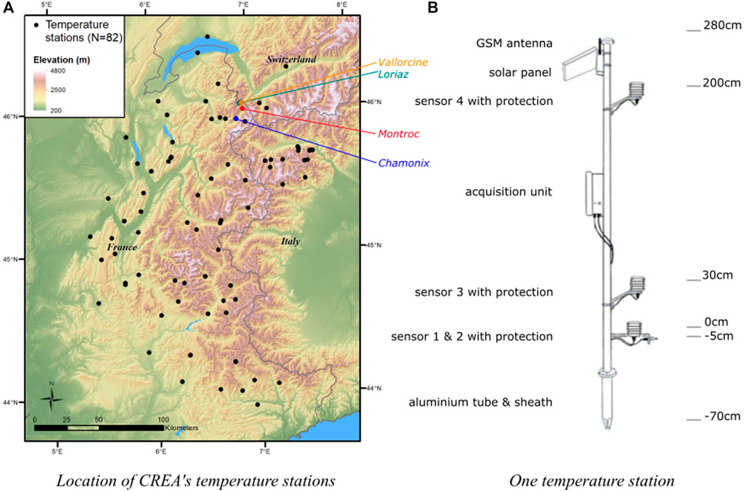
FIGURE 1. Location of the stations (A) and description of their components (B).
Stations are composed of a white 3.5 m aluminum tube, of which the first 70 cm are inserted into the soil through a sheath (Figure 1B). Their white color limits heating by sun rays and merges in the landscape, at least in winter. The components of the stations (solar panel, sensors, antenna) are made from Inox steel for rigidity and resistance to corrosion. Their shape is designed to avoid snow accumulation. Solar panels allow station electrical autonomy and a voltage regulator ensures battery recharge. Battery autonomy alone is around 60 days. Temperature stations have four “onewire” Dallas DS18B20 sensors inside brass cases embedded in a ventilated atmospheric shelter. Stacked PVC cups are resistant to ultraviolet radiation and allow air circulation, while protecting sensors from direct sun rays. Sensors are positioned at 5 cm below the soil surface, at the soil surface, 30 cm above the soil surface, and 2 m above ground (Figure 1B). These four heights were chosen according to species living conditions: the 2 m sensor gives information for tree and tall shrub canopy temperature conditions, the 30 cm for herbs and dwarf shrubs, and the 0 and −5 cm sensors give the temperature for short-stature alpine vegetation plant roots and soil fauna. The sensor located at −5 cm also informs us of the presence of snow. An electronic card ensures system functioning: measurements, data processing, storage and data transmission. Data are sent through the GPRS module integrated into the electronic card and uploaded to an FTP server. Sensors take a measurement every 15 min and data are sent to the server every hour.
Data were first screened using an automated script to remove erroneous measurements and date errors. We also manually checked data validity. We removed recurring errors such as strings of particular values known to be wrong, identical values recorded by the four sensors at the same time, and sudden variations. Finally, by comparing station data to S2M, we highlighted periods during which some stations had abnormal measurements, which we subsequently deleted.
When the missing data period was equal or inferior to 4 h, we used the R function “na.approx” from package zoo (Zeileis and Grothendieck, 2005) to interpolate missing values. At a given time, if sensor 1 or 2 (Figure 1B) had missing values, and sensor 3 recorded two following values inferior to 2°C, superior to −2°C and with a variance inferior to 0.2°C, we estimated that the missing values equaled zero, meaning that sensor 1, 2 and 3 were under the snow. Following the same rule applied to sensor 2, we completed sensor 1 missing values, and vice versa. For sensors 1, 2 and 3, if the 300 measures before and after a period of maximum 300 missing values, were inferior to 2°C and superior to −2°C, we estimated that missing values equaled 0°C.
Data processing was done with R version 3.3.3 (R Core Team, 2020).
We used daily mean air temperature values from the SAFRAN model developed by the French National Center of Meteorological Research (CNRM/CEN). SAFRAN is a meteorological analysis which combines output from a numerical weather prediction model and in situ observations (Durand et al., 1993; Vernay et al., 2021). SAFRAN predicts various meteorological variables at 1-hour time steps such as temperature, wind, precipitation and radiation. The SAFRAN-Crocus-MEPRA (S2M) model chain (Brun et al., 1989, 1992; Vionnet et al., 2013) predicts snow pack height and other physical properties based on meteorological inputs from SAFRAN. S2M outputs are generated for 23 alpine massifs throughout the French Alps, and further divided into 300 m elevation classes, six aspects (N, NE, E, SE, S, SW, W, and NW) and three slope classes (0, 20°, 40°). Vernay et al. (2021) define a massif as a conceptual object corresponding to a mountainous area (of about 1,000 km2 on average) over which the meteorological conditions are considered homogeneous at a given elevation. We did not consider different slopes as they only slightly influence temperature and snowpack values in the S2M analysis. Hence, we assigned stations to S2M elevation classes, by massif, for purposes of comparative analysis. We chose not to interpolate model values to the exact elevation of the stations, as the relationship between elevation and temperature is not always linear, for example in the case of temperature inversions.
We compared several seasonal indices known to influence species phenology, calculated from stations and S2M data. We also investigated whether species responses to climatic parameters depended on input data (station or S2M data). We carried out comparative analyses between 1 January 2006 and 1 August 2018. S2M models are only available in France, therefore we excluded Italian and Swiss stations from subsequent analyses. We also removed nine stations that were outside massifs defined in S2M.
We first calculated daily mean, minimum and maximum temperatures from the 2 m sensor of station data to compare them to S2M data. Daily values were only calculated when at least 80% of the daily measurements were available.
Chilling is defined as the frequency of days with a daily mean temperature
In relation to spring phenology of target tree species, we defined growing degree days (GDD) as the sum of daily air temperatures above a 0°C threshold between January 1st and April 1st (Asse et al., 2018). We calculated GDD using the 2 m sensor of each station and associated S2M class, for each year when all data were available from September January 1st and April 1st for at least 8 years.
We calculated the number of heat wave days for each station and year following the methods of Corona-Lozada et al. (2019). This method is based on the calculation of warm days and then heat waves. We counted the number of days presenting an air temperature above the 90th percentile, based on daily S2M temperature values for a 1981–2010 reference period. Heat waves are determined as episodes of at least three consecutive days above the daily temperature threshold. Lastly, we summed the number of heat waves for each year and station. We compared the number of heat waves between S2M and stations that presented at least five summers with complete data.
We compared snow melt-out dates estimated by S2M and stations. In the case of stations, we considered a snow layer to be present when soil temperature at −5 cm was stabilized around 0°C (±2°C) during 3 days, and the variance between mean soil temperature of these 3 consecutive days was inferior to 0.7°C (Reusser and Zehe, 2011; Schmid et al., 2012; Teubner et al., 2015). We determined the presence of a snow layer from S2M when snow height was
We compared snow melt-out dates between S2M and stations for which we could calculate snow melt-out date for at least 5 years (22 stations). Several stations were then excluded as they ran for less than 5 years, or had missing values during their running period. Winters were excluded when stations did not record temperature for at least 10 days, or their longest snow period ended with missing values.
We also visually observed snow presence on a daily basis in Chamonix (1,045 m) and Montroc (1,410 m) during the winter months (Figure 1).
We compared relationships between temperature (chilling and GDD) and budburst dates for five tree species, calculated using stations and S2M. We obtained budburst dates for ash (Fraxinus excelsior), spruce (Picea abies), hazel (Corylus avellana), birch (Betula pendula) and larch (Larix decidua) from the Phenoclim project (Phenoclim, 2020). We attributed observations to the closest stations when they were included within an observation perimeter of 15, 7.5, 3.75, or 1.9 km radius from the station and had a difference in altitude with the station inferior to 100 m. Several observation zones could be associated with the same station.
We investigated the effects of snow melt-out on common frog maximum egg-spawning date (Rana temporaria) using S2M and station datasets. The common frog egg-laying dates were noted for several ponds at Loriaz (1970 m) and Vallorcine (1,340 m, Figure 1A) by CREA Mont-Blanc employees and volunteers (Bison et al., 2021). We then calculated the maximum egg-spawning date as the date with the maximum number of spawn in the ponds.
We calculated the mean egg laying date of coal tits (Periparus ater) at two elevations (Vallorcine, 1,340 m and Loriaz, 1915 m; Figure 1) from weekly birdhouse observations (Bison et al., 2020). We assessed co-variation between egg laying date and snow melt-out date, and spring air temperature.
We computed linear regressions between indices calculated from S2M as the response variable and stations as the predictor, and calculated R.adj2 (adjusted R squared), RMSE (root mean squared error) and MAE (mean absolute error) of the regressions. When R.adj2 was superior to 0.70, we also used major axis (MA) estimation tests to calculate slopes of the regressions for each station (Warton et al., 2006), and the best-fit common regression slope among all stations, as well as confidence intervals (Warton and Weber, 2002). MA is relevant when comparing two datasets that both present potential errors (stations and S2M).
To investigate whether the quality of the regressions between daily means calculated from stations and data from S2M varied according to months, we calculated the R.adj2 of the regressions for each month and station. Relationships were tested only if at least 25 daily averages were available for the month, during 5 years, for each station.
We assessed differences between snow melt-out date calculated from both datasets, for each stations and massif in order to detect potential spatial variability in agreement between stations and S2M data. We then compared the beginning (onset) and end (melt-out date) of the snow covered period across visual observations, station and S2M data, at two sites in the Chamonix Mont-Blanc valley (Chamonix—1,050 m and Montroc—1,430 m), for each year, considering that visual observations were the reference (true value).
For each of the four perimeters considered (15, 7.5, 3.75, or 1.9 km radius), we computed linear mixed models testing the effects of GDD and chilling days on budburst dates of each species, considering stations as a random factor (as in Asse et al. (2018)), for a total of 28 stations. We then compared AIC between models computed with predictor variables calculated from station and S2M data. We also compared differences in AIC between models implemented with data coming from different observation perimeters to investigate whether station models had a better support when data were closer to the station.
We tested the relationship between the mean of the maximum egg-laying date for both sites, by year, and snow melt-out with the two datasets with linear models. Following Bison et al. (2020), we used linear models to evaluate how snow melt-out date and mean spring air temperature influenced the mean of laying date of coal tits at the two elevations, included as an interaction with the two others variables, using stations and S2M data.
Analyses were carried out with R (R Core Team, 2020) version 4.0.3 and packages smatr (Warton et al., 2012) and nlme (Pinheiro et al., 2020).
According to the MA test, slopes of the regressions between daily averages, chilling and GDD calculated from stations and S2M varied according to stations (Table 1).
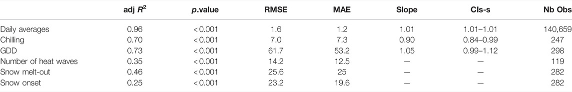
TABLE 1. Results from linear regressions between indices calculated from S2M and stations. adj R2 = adjusted R2, RMSE = Root mean squared error, MAE = Mean Absolute Error, Slope = best-fit common regression slope calculated from MA, CIs = 95% confidence intervals of the slopes, Nb Obs = Number of observations.
Figure 2 illustrates a typical year of data produced by an example station, with seasonal snow cover indicated by stable soil temperatures around 0°C and higher variability recorded by above-ground sensors.
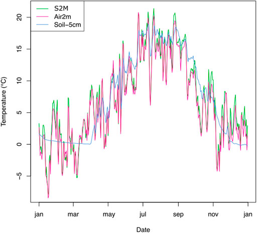
FIGURE 2. Temperatures measured from two sensors (−5 cm below soil surface and 2 m above the soil) of the station in Montroc and respective S2M air temperatures, during the year 2016.
Daily mean temperatures at 2 m recorded by stations were well correlated to air temperatures predicted by S2M each month (mean R.adj2 = 0.92 ± 0.06), with average slopes of 0.97 (±0.08) and a mean error of 0.02. However correlations were lower in winter (Figure 3).
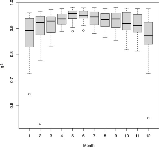
FIGURE 3. Adjusted R squared from regressions between daily average temperatures calculated from the stations and from S2M. Regressions were computed for each station and month.
In addition, daily minimum and maximum temperatures at 2 m recorded by stations were well correlated to minimum an maximum air temperatures predicted by S2M each month (mean R.adj2 = 0.83 ± 0.1, and mean R.adj2 = 0.77 ± 0.1), with average slopes of 0.91 (±0.07) and 0.97 (±0.1), and a mean error of 0.02 and 0.03, respectively. The average difference between minimum temperatures calculated from S2M and from stations was equal to 1.28°C, and −2.27°C for maximum temperatures.
The regression between the number of chilling days calculated from S2M and stations had a global R.adj2=0.73 (min = 0.58, max = 0.98) and a low dispersion (RMSE = 7, Table 1; Figure 4A).
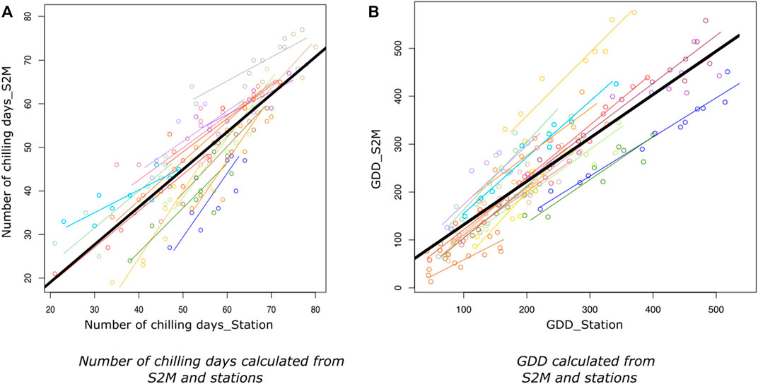
FIGURE 4. Relationship between number of chilling days (A) and growing degree days (B) calculated from S2M and from stations, with stations having at least 8 years with accurate data. Lines represent the linear regressions of the number of chilling days or GDD calculated from S2M as a function of chilling days or GDD calculated from stations, for each station. Colors represent stations. The black line corresponds to the linear model taking all stations together.
R.adj2 of the regressions between GDD calculated from station and S2M, for each station, varied from 0.75 to 0.97 (Figure 4B) with a global R.adj2=0.73 (Table 1).
The relationship between station and S2M data was weak (R.adj2 = 0.35, Table 1). Correlations between the number of heat wave days calculated from stations and S2M varied according to stations, with some stations even presenting a negative relationship (Figure 5). However, inter-annual patterns of warm summers were similar between data from stations and S2M with 2009, 2012 and 2017 standing out as exceptionally warm summers (Figure 6). Stations tended to estimate more heat waves than S2M (mean difference = 12 ±14 days).
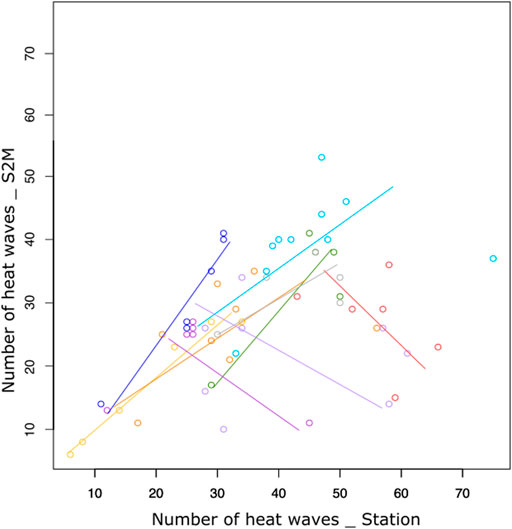
FIGURE 5. Number of days of heat waves calculated from stations and S2M for each station (colors) having at least five summers with complete data.
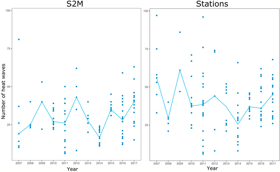
FIGURE 6. Number of heat waves calculated from each station (points) and median among all stations for each year (blue line).
Correlation strengths between station and S2M dates of snow onset and snow melt-out were low (R.adj2 = 0.25 and R.adj2 = 0.46, respectively), and presented high dispersion (RMSE > 20, Table 1).
Differences between S2M and station snow melt-out dates varied according to stations and years, with a maximum difference of 108 days. Snow melt-out dates calculated by stations were usually earlier than the ones assessed by S2M (average difference = 26 ±26 days). However, three stations from the Vercors exhibited consistently later snow melt-out in the case of stations compared to S2M (Figure 7).
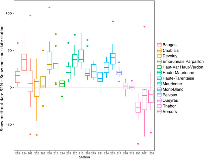
FIGURE 7. Boxplot of differences in snow melt-out date between S2M and stations for each station having at least 5 years with accurate data, divided by massif and by increasing order of elevation.
Snow onset in the fall calculated from S2M was in general closer to human observations than stations, while snow melt-out in the spring was usually estimated with a delay by S2M in comparison to stations and observations (Figure 8). Differences between observations, S2M and stations varied according to years.
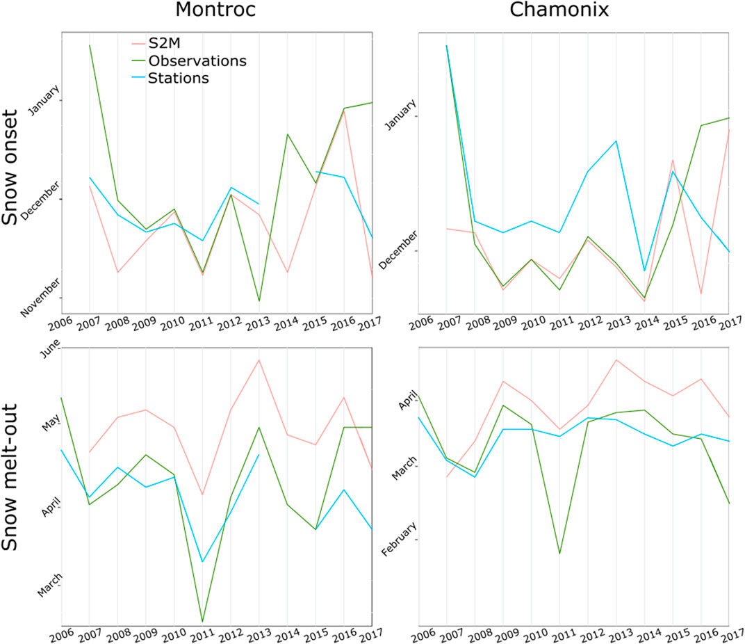
FIGURE 8. Beginning and ending of the longest period with a snow cover, according to S2M, stations and visual observations at Montroc and Chamonix.
The effects of chilling and GDD on budburst date for the five tree species were similar whether we used S2M or station data (Table 2). In both cases GDD had a significant effect on budburst date, whereas chilling had a significant effect on budburst date only for ash, and birch using station data, with a p.value < 0.05. Based on AIC differences between S2M and station models, support for models computed with S2M data decreased with the observation perimeter for birch, hazelnut and ash. Models based on station data had stronger support than the ones based on S2M data for spruce no matter the perimeter of observation. In contrast, there was more support for S2M models than station models concerning larch, and support increased with decreasing perimeter of observation.
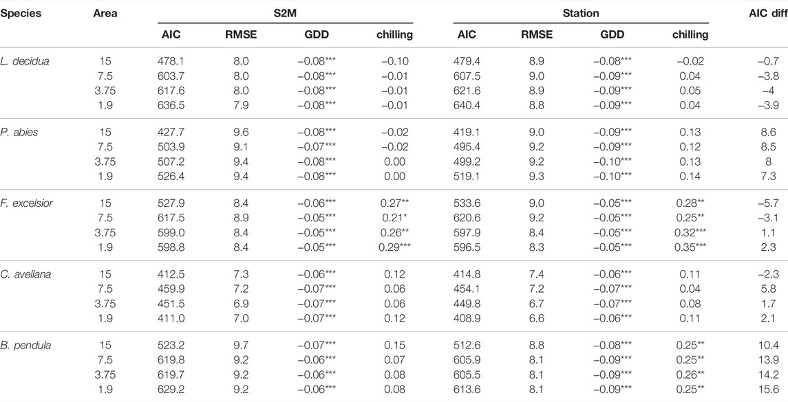
TABLE 2. Estimates and AIC from linear mixed models testing the effects of GDD and number of chilling days on five tree species budburst dates, using S2M or station data, and their AIC difference (S2M - station model). Models were tested with phenological data observed at a distance inferior to 15, 7.5, 3.75, and 1.9 km from the closest station. ***, **, * indicate statistical significance at p < 0.01, 0.05 and 0.10, respectively.
Snow melt-out and maximum egg-spawning dates were well correlated using S2M or station dates (R.adj2=0.63, p.value < 0.0001 and R.adj2=0.68, p.value < 0.0001, respectively). However, the common frog often laid its eggs before snow melt-out determined by S2M, which is impossible because ponds are not accessible. The maximum delay between egg-spawning date and snow melt-out date was 28 and 18 days in 2012, at low and high elevation, respectively (Figure 9).
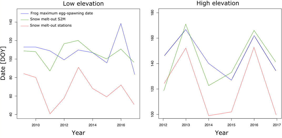
FIGURE 9. Maximum frog egg-spawning date and snow melt-out date estimated from stations and S2M, in julian days, according to years, at low and high elevation.
The model testing the effects of spring temperature and snow melt-out date on coal tits laying date had a lower AIC using station data (AIC = 86.3) and a higher R.adj2 (R.adj2=0.66) than the model implemented with S2M data (AIC = 92.5, R.adj2=0.43). In both cases, snow melt-out did not have an effect on laying date (p.value > 0.1), but spring temperature had a significant effect using station data (p.value = 0.04) and a non significant effect using S2M data (p.value = 0.09).
Quantifying bioclimatic drivers in mountains at temporal and spatial scales relevant to biological activity remains a long-standing and persistent challenge for ecologists. While most species distribution models are based on kilometer-resolution gridded climate data sets (Schorr et al., 2012; Karger et al., 2017; Cornes et al., 2018), several studies have highlighted the significant influence of microclimate on alpine plant composition (Scherrer and Körner, 2011; Carbognani et al., 2016), distribution (Randin et al., 2009; Graae et al., 2018) and phenology (Wang et al., 2014), but see (Zellweger et al., 2019). Here, in order to understand and predict species phenological responses to climate, we assessed the relevance of using bioclimatic variables derived from either local temperature stations or obtained from a mountain range-scale meteorological model (S2M). Several indices showed little sensitivity to data-source while others presented significant differences according to data origin, with strong implications for resulting relationships between climate variability and species phenology.
We found the strongest agreement between daily average temperatures measured by the two datasets. Although GDD and chilling days, which are based on temperature averages, also showed fairly strong agreement between the two datasets, the introduction of a threshold reduced correlation strength as compared to average temperatures. Indeed, on average, Vernay et al. (2021) highlighted that SAFRAN minimum temperature is 0.2°C higher and the maximum temperature is 0.4°C lower than the absolute value of hourly temperatures. We found even stronger differences, with an average difference of 1.3°C between S2M minimum temperatures and stations, and of −2.27°C between S2M maximum temperatures and stations. These variations in temperature above or below the threshold level could therefore lead to pronounced shifts in the resulting index. Validation of models using daily or monthly averages, which is common practice (Quintana-Segui et al., 2008; Fick and Hijmans, 2017; Caillouet et al., 2019), can thus mask more subtle differences in absolute temperature values, which may be significant for the biological functioning of organisms.
Certain bioclimatic indices such as snow onset and melt-out dates, or heat wave index, showed strong differences depending on data source (S2M or stations). These indices also depend on thresholds, either above a certain reference air temperature or above a minimum number of days estimated with snow on the ground. The heat wave index was particularly sensitive to initial differences in air temperature values, given that it is based on both the magnitude and duration of events. Temperature estimation by S2M leads to a mean deviation of −0.4°C on maximum temperature which can partly explain the lower number of heat waves calculated by S2M (Vernay et al., 2021). Moreover, differences could have been exacerbated owing to the fact that the reference threshold (90th percentile) for heat waves were calculated only from S2M data, as station data did not have sufficient historic depth. Collectively, our results suggest using caution when applying modeled data to estimate bioclimatic variables that are threshold dependent, both from the standpoint of statistical performance and for determining temperature based physiological thresholds that rely on absolute values.
Modelling spatial variability in snow cover duration in complex mountain terrain is notoriously difficult, and is a topic of ongoing research (Vionnet et al., 2021). Estimating snow presence from sub-surface soil temperature is known to be a reliable local measure (Reusser and Zehe, 2011; Schmid et al., 2012; Teubner et al., 2015), and in our case proved to be quite consistent with visual observations. However, given that snow onset was often estimated later from stations compared to S2M, it is possible that stations exhibited a lag between snow onset and measured temperatures around 0°C. In addition, snow melt-out was usually predicted later by S2M than stations. Our results are in accordance with Vionnet et al. (2016) who found that S2M is adequate to predict snow onset but can make predictions that are 25 days earlier or later than actual observations of snow offset dates.
Pronounced differences in snow cover duration of up to 1 month or more between stations and S2M data are, in the end, not so surprising, considering that S2M provides outputs for broad topographic classes. Previous work indicated differences of up to a month or more in snow cover duration within a 300 m band of elevation based on meso-topography and local heterogeneity in snow cover accumulation and ablation (Carlson et al., 2015). Moreover, S2M underestimates snow ablation by wind as it is a local phenomena, as well as strong snowpack melting (Quéno et al., 2016; Vionnet et al., 2016). Snow presence is highly influenced by micro-topography and underlying or adjacent plant canopies (Sturm et al., 2001; Revuelto et al., 2015; Belke-Brea et al., 2020) and complex phenomena such as wind transport and redistribution of snow due to avalanches (Vionnet et al., 2021). All of these challenges make it difficult to precisely predict local snowpack conditions using models (Ford et al., 2013; Vionnet et al., 2019). Finally, snow predictions from S2M result from both SAFRAN and CROCUS outputs, and thereby accumulate errors from both models (Vernay et al., 2021). Quantifying spatial variability in snow cover duration remains a challenge for ecologists seeking to predict species distribution and phenology at specific locations, particularly in forested environments where snow mapping approaches based on optical remote sensing are less effective (Dedieu et al., 2016).
In accordance with results presented above, statistical models testing the effects of chilling and GDD on budburst dates led to similar results using either dataset. Overall, phenological and climate indices followed the same directional trends across years. However, station models out-performed S2M models when we decreased the acceptable distance between budburst observations stations, which underscored the relevance of local climate data for predicting local biological responses.
It is worth mentioning that larch was an important exception to this pattern, with models consistently showing increased performance in the case of S2M predictors regardless of buffer size. One possible explanation could be a lack of temperature stations located along elevation gradients, which would be necessary in order to predict heterogeneous budburst responses to warming with respect to elevation. Given that larch phenology is understood to be advancing at higher elevations and experiencing delay at lower elevations (Asse et al., 2018; Vitasse et al., 2018), a single temperature station located in the middle of the gradient might blur the signal and lead to a weaker result compared to S2M temperature values consistently available for 300 m elevation bands. However, Lembrechts et al. (2019) also found that species distribution models are better explained by local temperatures with some species being exceptions. In general and with respect to predicting tree budburst date relative to climate, we found S2M data to be quite reliable and sufficient for assessing directional long-term trends.
In the case of coal tits and frogs, models yielded similar statistical results, but mechanisms could not always be biologically explained by both datasets. For instance, egg-spawning dates of frogs usually occurred before dates of snow melt-out estimated by S2M, in contrast to snow melt-out consistently preceding egg-spawning when snow cover predictors were derived from station data. Given the observed link between snow melt-out and rapidly ensuing spawning of the European common frog in mountain habitats (Bison et al., 2021), in order to avoid erroneous predictions, it seems important to have not only a statistical correlation but also an ecologically relevant estimate of local snow melt-out timing. In many cases, accurate meteorological and snowpack data appear essential not only to understand phenological mechanisms, but also in order to predict non-linear and threshold-based responses to climate variability and change.
We show that the choice of broad scale or local climatic datasets depends on the initial questions and the biological model. Stations provide precise data for a particular site with high temporal resolution (15 min) that allows for calculating complex bioclimatic variables. The four sensors give measurements at different heights making pertinent the use of station data to link temperatures to surrounding biodiversity. This feature is of particular interest when studying temperature effects on biodiversity as air and soil temperatures can significantly differ (Kollas et al., 2014; Shen et al., 2020, 2022b), with sometimes mean annual temperature differences up to 10°C (Lembrechts et al., 2021). The −5 cm sensor can inform us about living conditions of roots and soil invertebrates, and is used to estimate snow presence, the 0 and 30 cm sensors can be used to link temperatures to herbaceous vegetation or ground dwelling animals, the 2 m sensor is helpful at studying effects of air temperature on tree growth. The higher precision of station data helps in understanding actual mechanisms affecting species phenology (based on temperature thresholds, or snow cover duration), as opposed to simply studying relative trends in climate and species’ response over time. Moreover, we found that agreement between station and climate model outputs fluctuates according to season and local factors. Temporal variation in differences between datasets is difficult to understand and changes according to stations irrespective of elevation or slope. When comparing S2M daily temperature averages to station data at the scale of France, Quintana-Segui et al. (2008) and Caillouet et al. (2019) also highlighted spatial and seasonal variations in S2M biases, and reported a similar RMSE as compared to our study (1.5°C). One explanation could be the number of stations used as input for the S2M analysis that varied according to massif, elevation and years, and the size of the considered homogeneous units [massif and 300 m elevation classes, Vionnet et al. (2016); Vernay et al. (2021)]. Moreover, physical parametrisation and horizontal resolution of the model input for S2M changed over time. These temporal changes had particularly strong effects on winter trend biases (Vernay et al., 2021). In winter, the climate is also more variable because of greater wind, and possible temperature inversions (Vitasse et al., 2017). Accordingly, we observe greater differences between datasets during the winter months. Due to these considerations, we did not detect a perfect linear relationship between indices calculated from both datasets. Species are sensitive to small changes in temperature, therefore differences between S2M data and absolute values can have strong implications in the understanding of species responses to climate. We then suggest that station data are more accurate for the study of local phenomena, and especially of biological processes.
Given the uncertainties of climate model predictions, we recommend the use of local climate stations when possible, however station data also present some limitations. The downsides of station data include 1) inevitably limited spatial coverage, 2) often limited historical depth, which is typically key for long-term studies with respect to climate, 3) frequent missing values due to technical malfunctions and 4) high cost, both financial and in terms of human resources, of installation and maintenance, 5) impossibility to make predictions for the future. Given these constraints and in light of our results, we consider widely available and state-of-the-art reanalysis data to be appropriate for assessing long-term trends in species phenological responses at broad scales, such as tree budburst, with respect to climate variation. In contrast, we conclude that in situ temperature data remains preferable for assessing physiologically-based hypotheses tied to inter-annual climate variability, especially in alpine ecosystems and when using bioclimatic variables based on snow cover duration and temperature thresholds.
The raw data supporting the conclusion of this article will be made available by the authors, without undue reservation.
AD conceived of the presented idea and developped the Phenoclim project. IL preformed the statistical analyses and wrote the manuscript with support from BC and NY. NY supervised the project. All authors discussed the results and contributed to the final manuscript.
The authors declare that the research was conducted in the absence of any commercial or financial relationships that could be construed as a potential conflict of interest.
All claims expressed in this article are solely those of the authors and do not necessarily represent those of their affiliated organizations, or those of the publisher, the editors and the reviewers. Any product that may be evaluated in this article, or claim that may be made by its manufacturer, is not guaranteed or endorsed by the publisher.
This project was implemented thanks to assistance from several partners including technical support (SOMFY, ORANGE), professional project (ADISON), the participation of school groups (CECAM: lycée professionnel, Saint Jeoires, LPVA—lycée professionnel de la vallée de l’Arve, Cluses, LCP—lycée Charles Poncet, Cluses), and frequent help from individual volunteers, especially Gérard Cordier, Patrick Magnin and Alain Debourg. ORANGE also developed the interface used for data processing. We would also like to thank all participants who carried out observations of tree phenology for the Phenoclim program including staff from national and regional parks, natural reserves, associations, school groups and individual citizens. The S2M data are provided by Météo-France—CNRS, CNRM Centre d’Etudes de la Neige, through AERIS. We would like to thank Samuel Morin, from the CEN Meteo-France-CNRS for his helpfull comments.
The Supplementary Material for this article can be found online at: https://www.frontiersin.org/articles/10.3389/feart.2022.912048/full#supplementary-material
Asse, D., Chuine, I., Vitasse, Y., Yoccoz, N. G., Delpierre, N., Badeau, V., et al. (2018). Warmer Winters Reduce the Advance of Tree Spring Phenology Induced by Warmer Springs in the Alps. Agric. For. Meteorology 252, 220–230. doi:10.1016/j.agrformet.2018.01.030
Asse, D., Randin, C. F., Bonhomme, M., Delestrade, A., and Chuine, I. (2020). Process-based Models Outcompete Correlative Models in Projecting Spring Phenology of Trees in a Future Warmer Climate. Agric. For. Meteorology 285-286, 107931. doi:10.1016/j.agrformet.2020.107931
Belke-Brea, M., Domine, F., Barrere, M., Picard, G., and Arnaud, L. (2020). Impact of Shrubs on Winter Surface Albedo and Snow Specific Surface Area at a Low Arctic Site: In Situ Measurements and Simulations. J. Clim. 33, 597–609.
Bison, M., Yoccoz, N. G., Carlson, B., Klein, G., Laigle, I., Van Reeth, C., et al. (2020). Best Environmental Predictors of Breeding Phenology Differ with Elevation in a Common Woodland Bird Species. Ecol. Evol. 10, 10219–10229. doi:10.1002/ece3.6684
Bison, M., Yoccoz, N. G., Carlson, B., Klein, G., Laigle, I., Van Reeth, C., et al. (2021). Earlier Snowmelt Advances Breeding Phenology of the Common Frog (rana Temporaria) but Increases the Risk of Frost Exposure and Drought. Front. Ecol. Evol..
Bliss, L. (1962). Adaptations of Arctic and Alpine Plants to Environmental Conditions. Arctic 15, 117–144. doi:10.14430/arctic3564
Brun, E., David, P., Sudul, M., and Brunot, G. (1992). A Numerical Model to Simulate Snow-Cover Stratigraphy for Operational Avalanche Forecasting. J. Glaciol. 38, 13–22. doi:10.3189/s0022143000009552
Brun, E., Martin, Ε., Simon, V., Gendre, C., and Coleou, C. (1989). An Energy and Mass Model of Snow Cover Suitable for Operational Avalanche Forecasting. J. Glaciol. 35, 333–342. doi:10.3189/s0022143000009254
Brun, P., Thuiller, W., Chauvier, Y., Pellissier, L., Wüest, R. O., Wang, Z., et al. (2020). Model Complexity Affects Species Distribution Projections under Climate Change. J. Biogeogr. 47, 130–142. doi:10.1111/jbi.13734
Caillouet, L., Vidal, J.-P., Sauquet, E., Graff, B., and Soubeyroux, J.-M. (2019). Scope Climate: A 142-year Daily High-Resolution Ensemble Meteorological Reconstruction Dataset over france. Earth Syst. Sci. Data 11, 241–260. doi:10.5194/essd-11-241-2019
Carbognani, M., Bernareggi, G., Perucco, F., Tomaselli, M., and Petraglia, A. (2016). Micro-climatic Controls and Warming Effects on Flowering Time in Alpine Snowbeds. Oecologia 182, 573–585. doi:10.1007/s00442-016-3669-3
Carlson, B. Z., Choler, P., Renaud, J., Dedieu, J.-P., and Thuiller, W. (2015). Modelling Snow Cover Duration Improves Predictions of Functional and Taxonomic Diversity for Alpine Plant Communities. Ann. Bot. 116, 1023–1034. doi:10.1093/aob/mcv041
Choler, P. (2005). Consistent Shifts in Alpine Plant Traits along a Mesotopographical Gradient. Arct. Antarct. Alp. Res. 37, 444–453. doi:10.1657/1523-0430(2005)037[0444:csiapt]2.0.co;2
Choler, P. (2018). Winter Soil Temperature Dependence of Alpine Plant Distribution: Implications for Anticipating Vegetation Changes under a Warming Climate. Perspect. Plant Ecol. Evol. Syst. 30, 6–15. doi:10.1016/j.ppees.2017.11.002
Cook, B. I., Wolkovich, E. M., and Parmesan, C. (2012). Divergent Responses to Spring and Winter Warming Drive Community Level Flowering Trends. Proc. Natl. Acad. Sci. U.S.A. 109, 9000–9005. doi:10.1073/pnas.1118364109
Cornes, R. C., van der Schrier, G., van den Besselaar, E. J. M., and Jones, P. D. (2018). An Ensemble Version of the E-Obs Temperature and Precipitation Data Sets. J. Geophys. Res. Atmos. 123, 9391–9409. doi:10.1029/2017jd028200
Corona-Lozada, M. C., Morin, S., and Choler, P. (2019). Drought Offsets the Positive Effect of Summer Heat Waves on the Canopy Greenness of Mountain Grasslands. Agric. For. Meteorology 276-277, 107617. doi:10.1016/j.agrformet.2019.107617
Cremonese, E., Filippa, G., Galvagno, M., Siniscalco, C., Oddi, L., Morra di Cella, U., et al. (2017). Heat Wave Hinders Green Wave: The Impact of Climate Extreme on the Phenology of a Mountain Grassland. Agric. For. Meteorology 247, 320–330. doi:10.1016/j.agrformet.2017.08.016
Dantec, C. F., Vitasse, Y., Bonhomme, M., Louvet, J.-M., Kremer, A., and Delzon, S. (2014). Chilling and Heat Requirements for Leaf Unfolding in European Beech and Sessile Oak Populations at the Southern Limit of Their Distribution Range. Int. J. Biometeorol. 58, 1853–1864. doi:10.1007/s00484-014-0787-7
Dedieu, J.-P., Carlson, B., Bigot, S., Sirguey, P., Vionnet, V., and Choler, P. (2016). On the Importance of High-Resolution Time Series of Optical Imagery for Quantifying the Effects of Snow Cover Duration on Alpine Plant Habitat. Remote Sens. 8, 481. doi:10.3390/rs8060481
Durand, Y., Brun, E., Merindol, L., Guyomarc'h, G., Lesaffre, B., and Martin, E. (1993). A Meteorological Estimation of Relevant Parameters for Snow Models. A. Glaciol. 18, 65–71. doi:10.1017/s0260305500011277
Espunyes, J., Serrano, E., Chaves, S., Bartolomé, J., Menaut, P., Albanell, E., et al. (2022). Positive Effect of Spring Advance on the Diet Quality of an Alpine Herbivore. Integr. Zool. 17, 78–92. doi:10.1111/1749-4877.12572
Fick, S. E., and Hijmans, R. J. (2017). WorldClim 2: New 1‐km Spatial Resolution Climate Surfaces for Global Land Areas. Int. J. Climatol. 37, 4302–4315. doi:10.1002/joc.5086
Ford, K. R., Ettinger, A. K., Lundquist, J. D., Raleigh, M. S., and Hille Ris Lambers, J. (2013). Spatial Heterogeneity in Ecologically Important Climate Variables at Coarse and Fine Scales in a High-Snow Mountain Landscape. PLOS ONE 8, e65008–13. doi:10.1371/journal.pone.0065008
Francon, L., Corona, C., Till‐Bottraud, I., Carlson, B. Z., and Stoffel, M. (2020). Some (Do Not) like it Hot: Shrub Growth Is Hampered by Heat and Drought at the Alpine Treeline in Recent Decades. Am. J. Bot. 107, 607–617. doi:10.1002/ajb2.1459
Giaccone, E., Luoto, M., Vittoz, P., Guisan, A., Mariéthoz, G., and Lambiel, C. (2019). Influence of Microclimate and Geomorphological Factors on Alpine Vegetation in the Western Swiss Alps. Earth Surf. Process. Landforms 44, 3093–3107. doi:10.1002/esp.4715
Graae, B. J., Vandvik, V., Armbruster, W. S., Eiserhardt, W. L., Svenning, J.-C., Hylander, K., et al. (2018). Stay or Go - How Topographic Complexity Influences Alpine Plant Population and Community Responses to Climate Change. Perspect. Plant Ecol. Evol. Syst. 30, 41–50. doi:10.1016/j.ppees.2017.09.008
Jabis, M. D., Winkler, D. E., and Kueppers, L. M. (2020). Warming Acts through Earlier Snowmelt to Advance but Not Extend Alpine Community Flowering. Ecology 101, e03108. doi:10.1002/ecy.3108
Jonas, T., Rixen, C., Sturm, M., and Stoeckli, V. (2008). How Alpine Plant Growth Is Linked to Snow Cover and Climate Variability. J. Geophys. Res. Biogeosciences 113. doi:10.1029/2007jg000680
Karger, D. N., Conrad, O., Böhner, J., Kawohl, T., Kreft, H., Soria-Auza, R. W., et al. (2017). Climatologies at High Resolution for the Earth's Land Surface Areas. Sci. Data 4. doi:10.1038/sdata.2017.122
Klein, G., Vitasse, Y., Rixen, C., Marty, C., and Rebetez, M. (2016). Shorter Snow Cover Duration since 1970 in the Swiss Alps Due to Earlier Snowmelt More Than to Later Snow Onset. Clim. Change 139, 637–649.
Kollas, C., Randin, C. F., Vitasse, Y., and Körner, C. (2014). How Accurately Can Minimum Temperatures at the Cold Limits of Tree Species Be Extrapolated from Weather Station Data? Agric. For. Meteorology 184, 257–266. doi:10.1016/j.agrformet.2013.10.001
Körner, C., and Hiltbrunner, E. (2021). Why Is the Alpine Flora Comparatively Robust against Climatic Warming? Diversity 13, 383. doi:10.3390/d13080383
Körner, C., Riedl, S., Keplinger, T., Richter, A., Wiesenbauer, J., Schweingruber, F., et al. (2019). Life at 0 °C: the Biology of the Alpine Snowbed Plant Soldanella Pusilla. Alp. Bot. 129, 63–80. doi:10.1007/s00035-019-00220-8
Lembrechts, J. J., Lenoir, J., Roth, N., Hattab, T., Milbau, A., Haider, S., et al. (2019). Comparing Temperature Data Sources for Use in Species Distribution Models: From In‐situ Logging to Remote Sensing. Glob. Ecol. Biogeogr. 28, 1578–1596. doi:10.1111/geb.12974
Lembrechts, J. J., van den Hoogen, J., Aalto, J., Ashcroft, M. B., De Frenne, P., Kemppinen, J., et al. (2021). Global Maps of Soil Temperature. Glob. Change Biol. doi:10.1111/gcb.16060
Löffler, J. (2007). The Influence of Micro-climate, Snow Cover, and Soil Moisture on Ecosystem Functioning in High Mountains. J. Geogr. Sci. 17, 3–19. doi:10.1007/s11442-007-0003-3
Marumo, E., Takagi, K., and Makoto, K. (2020). Timing of Bud Burst of Smaller Individuals Is Not Always Earlier Than that of Larger Trees in a Cool-Temperate Forest with Heavy Snow. J. For. Res. 25, 285–290. doi:10.1080/13416979.2020.1753279
Melin, M., Mehtätalo, L., Helle, P., Ikonen, K., and Packalen, T. (2020). Decline of the Boreal Willow Grouse (Lagopus Lagopus) Has Been Accelerated by More Frequent Snow-free Springs. Sci. Rep. 10. doi:10.1038/s41598-020-63993-7
Orsenigo, S., Mondoni, A., Rossi, G., and Abeli, T. (2014). Some like it Hot and Some like it Cold, but Not Too Much: Plant Responses to Climate Extremes. Plant Ecol. 215, 677–688. doi:10.1007/s11258-014-0363-6
Pellerin, M., Delestrade, A., Mathieu, G., Rigault, O., and Yoccoz, N. G. (2012). Spring Tree Phenology in the Alps: Effects of Air Temperature, Altitude and Local Topography. Eur. J. For. Res. 131, 1957–1965. doi:10.1007/s10342-012-0646-1
Petraglia, A., Tomaselli, M., Petit Bon, M., Delnevo, N., Chiari, G., and Carbognani, M. (2014). Responses of Flowering Phenology of Snowbed Plants to an Experimentally Imposed Extreme Advanced Snowmelt. Plant Ecol. 215, 759–768. doi:10.1007/s11258-014-0368-1
Phenoclim, C. (2020). Phenoclim les sciences participatives en montagne, 2020. Availableat: https://phenoclim.org/fr (Accessed 12 16.
Pinheiro, J., Bates, D., DebRoy, S., Sarkar, D., and Core Team, R. (2020). Nlme: Linear And Nonlinear Mixed Effects Models. R Package Version 3, 1–151.
Quéno, L., Vionnet, V., Dombrowski-Etchevers, I., Lafaysse, M., Dumont, M., and Karbou, F. (2016). Snowpack Modelling in the Pyrenees Driven by Kilometric-Resolution Meteorological Forecasts. Cryosphere 10, 1571–1589. doi:10.5194/tc-10-1571-2016
Quintana-Seguí, P., Le Moigne, P., Durand, Y., Martin, E., Habets, F., Baillon, M., et al. (2008). Analysis of Near-Surface Atmospheric Variables: Validation of the Safran Analysis over france. J. Appl. meteorology Climatol. 47, 92–107. doi:10.1175/2007jamc1636.1
R Core Team (2020). R: A Language and Environment for Statistical Computing. Vienna, Austria: R Foundation for Statistical Computing.
Randin, C. F., Engler, R., Normand, S., Zappa, M., Zimmermann, N. E., Pearman, P. B., et al. (2009). Climate Change and Plant Distribution: Local Models Predict High-Elevation Persistence. Glob. change Biol. 15, 1557–1569. doi:10.1111/j.1365-2486.2008.01766.x
Reusser, D. E., and Zehe, E. (2011). Low-cost Monitoring of Snow Height and Thermal Properties with Inexpensive Temperature Sensors. Hydrol. Process. 25, 1841–1852.
Revuelto, J., López-Moreno, J. I., Azorin-Molina, C., and Vicente-Serrano, S. M. (2015). Canopy Influence on Snow Depth Distribution in a Pine Stand Determined from Terrestrial Laser Data. Water Resour. Res. 51, 3476–3489.
Scherrer, D., and Körner, C. (2011). Topographically Controlled Thermal-Habitat Differentiation Buffers Alpine Plant Diversity against Climate Warming. J. Biogeogr. 38, 406–416. doi:10.1111/j.1365-2699.2010.02407.x
Schmid, M.-O., Gubler, S., Fiddes, J., and Gruber, S. (2012). Inferring Snowpack Ripening and Melt-Out from Distributed Measurements of Near-Surface Ground Temperatures. Cryosphere 6, 1127–1139. doi:10.5194/tc-6-1127-2012
Schorr, G., Holstein, N., Pearman, P. B., Guisan, A., and Kadereit, J. W. (2012). Integrating Species Distribution Models (SDMs) and Phylogeography for Two Species of AlpinePrimula. Ecol. Evol. 2, 1260–1277. doi:10.1002/ece3.100
Shen, M., Piao, S., Chen, X., An, S., Fu, Y. H., Wang, S., et al. (2016). Strong Impacts of Daily Minimum Temperature on the Green-Up Date and Summer Greenness of the Tibetan Plateau. Glob. Change Biol. 22, 3057–3066. doi:10.1111/gcb.13301
Shen, X., Liu, B., Henderson, M., Wang, L., Jiang, M., and Lu, X. (2022a). Vegetation Greening, Extended Growing Seasons, and Temperature Feedbacks in Warming Temperate Grasslands of china. J. Clim., 1–51. doi:10.1175/jcli-d-21-0325.1
Shen, X., Liu, B., Henderson, M., Wang, L., Wu, Z., Wu, H., et al. (2018). Asymmetric Effects of Daytime and Nighttime Warming on Spring Phenology in the Temperate Grasslands of china. Agric. For. Meteorology 259, 240–249. doi:10.1016/j.agrformet.2018.05.006
Shen, X., Liu, B., Jiang, M., and Lu, X. (2020). Marshland Loss Warms Local Land Surface Temperature in china. Geophys. Res. Lett. 47, e2020GL087648. doi:10.1029/2020gl087648
Shen, X., Liu, Y., Liu, B., Zhang, J., Wang, L., Lu, X., et al. (2022b). Effect of Shrub Encroachment on Land Surface Temperature in Semi-arid Areas of Temperate Regions of the Northern Hemisphere. Agric. For. Meteorology 320, 108943.
Sturm, M., Holmgren, J., McFadden, J. P., Liston, G. E., Chapin, F. S., and Racine, C. H. (2001). Snow-Shrub Interactions in Arctic Tundra: A Hypothesis with Climatic Implications. J. Clim. 14, 336–344. doi:10.1175/1520-0442(2001)014<0336:ssiiat>2.0.co;2
Suding, K. N., Farrer, E. C., King, A. J., Kueppers, L., and Spasojevic, M. J. (2015). Vegetation Change at High Elevation: Scale Dependence and Interactive Effects on Niwot Ridge. Plant Ecol. Divers. 8, 713–725.
Teubner, I. E., Haimberger, L., and Hantel, M. (2015). Estimating Snow Cover Duration from Ground Temperature. J. Appl. Meteorology Climatol. 54, 959–965. doi:10.1175/jamc-d-15-0006.1
Thornton, J. M., Pepin, N., Shahgedanova, M., and Adler, C. (2022). Coverage of In Situ Climatological Observations in the World’s Mountains. Front. Clim. 4. doi:10.3389/fclim.2022.814181
Vernay, M., Lafaysse, M., Monteiro, D., Hagenmuller, P., Nheili, R., Samacoïts, R., et al. (2021). The S2m Meteorological and Snow Cover Reanalysis over the French Mountainous Areas, Description and Evaluation (1958–2020). Earth Syst. Sci. Data Discuss., 1–36.
Vionnet, V., Dombrowski-Etchevers, I., Lafaysse, M., Quéno, L., Seity, Y., and Bazile, E. (2016). Numerical Weather Forecasts at Kilometer Scale in the French Alps: Evaluation and Application for Snowpack Modeling. J. Hydrometeorol. 17, 2591–2614. doi:10.1175/jhm-d-15-0241.1
Vionnet, V., Guyomarc’h, G., Naaim Bouvet, F., Martin, E., Durand, Y., Bellot, H., et al. (2013). Occurrence of Blowing Snow Events at an Alpine Site over a 10-year Period: Observations and Modelling. Adv. water Resour. 55, 53–63. doi:10.1016/j.advwatres.2012.05.004
Vionnet, V., Marsh, C. B., Menounos, B., Gascoin, S., Wayand, N. E., Shea, J., et al. (2021). Multi-scale Snowdrift-Permitting Modelling of Mountain Snowpack. Cryosphere 15, 743–769. doi:10.5194/tc-15-743-2021
Vionnet, V., Six, D., Auger, L., Dumont, M., Lafaysse, M., Quéno, L., et al. (2019). Sub-kilometer Precipitation Datasets for Snowpack and Glacier Modeling in Alpine Terrain. Front. Earth Sci. 7, 182. doi:10.3389/feart.2019.00182
Vitasse, Y., Bottero, A., Cailleret, M., Bigler, C., Fonti, P., Gessler, A., et al. (2019). Contrasting Resistance and Resilience to Extreme Drought and Late Spring Frost in Five Major European Tree Species. Glob. Chang. Biol. 25, 3781–3792. doi:10.1111/gcb.14803
Vitasse, Y., Baumgarten, F., Zohner, C. M., Kaewthongrach, R., Fu, Y. H., Walde, M. G., et al. (2021). Impact of Microclimatic Conditions and Resource Availability on Spring and Autumn Phenology of Temperate Tree Seedlings. New Phytol. 232, 537–550. doi:10.1111/nph.17606
Vitasse, Y., Klein, G., Kirchner, J. W., and Rebetez, M. (2017). Intensity, Frequency and Spatial Configuration of Winter Temperature Inversions in the Closed La Brevine Valley, Switzerland. Theor. Appl. Climatol. 130, 1073–1083. doi:10.1007/s00704-016-1944-1
Vitasse, Y., Signarbieux, C., and Fu, Y. H. (2018). Global Warming Leads to More Uniform Spring Phenology across Elevations. Proc. Natl. Acad. Sci. U.S.A. 115, 1004–1008. doi:10.1073/pnas.1717342115
Wang, T., Ottlé, C., Peng, S., Janssens, I. A., Lin, X., Poulter, B., et al. (2014). The Influence of Local Spring Temperature Variance on Temperature Sensitivity of Spring Phenology. Glob. Change Biol. 20, 1473–1480. doi:10.1111/gcb.12509
Warton, D. I., Wright, I. J., Falster, D. S., and Westoby, M. (2006). Bivariate Line-Fitting Methods for Allometry. Biol. Rev. Camb Philos. Soc. 81, 259–291. doi:10.1017/S1464793106007007
Warton, D. I., Duursma, R. A., Falster, D. S., and Taskinen, S. (2012). Smatr 3 - an R Package for Estimation and Inference about Allometric Lines. Methods Ecol. Evol. 3, 257–259. doi:10.1111/j.2041-210x.2011.00153.x
Warton, D. I., and Weber, N. C. (2002). Common Slope Tests for Bivariate Errors-In-Variables Models. Biom. J. 44, 161–174. doi:10.1002/1521-4036(200203)44:2<161::aid-bimj161>3.0.co;2-n
Xie, J., Hüsler, F., de Jong, R., Chimani, B., Asam, S., Sun, Y., et al. (2021). Spring Temperature and Snow Cover Climatology Drive the Advanced Springtime Phenology (1991–2014) in the European Alps. J. Geophys. Res. Biogeosciences, e2020JG006150.
Zeileis, A., and Grothendieck, G. (2005). zoo:S3Infrastructure for Regular and Irregular Time Series. J. Stat. Soft. 14, 1–27. doi:10.18637/jss.v014.i06
Zellweger, F., De Frenne, P., Lenoir, J., Rocchini, D., and Coomes, D. (2019). Advances in Microclimate Ecology Arising from Remote Sensing. Trends Ecol. Evol. 34, 327–341. doi:10.1016/j.tree.2018.12.012
Keywords: temperature, Alps, mountain, phenology, climate, Rana temporaria, Periparus ater, trees
Citation: Laigle I, Carlson BZ, Delestrade A, Bison M, Van Reeth C and Yoccoz NG (2022) In-situ Temperature Stations Elucidate Species’ Phenological Responses to Climate in the Alps, but Meteorological and Snow Reanalysis Facilitates Broad Scale and Long-Term Studies. Front. Earth Sci. 10:912048. doi: 10.3389/feart.2022.912048
Received: 03 April 2022; Accepted: 08 June 2022;
Published: 22 July 2022.
Edited by:
Binhui Liu, Northeast Forestry University, ChinaReviewed by:
Xiangjin Shen, Northeast Institute of Geography and Agroecology (CAS), ChinaCopyright © 2022 Laigle, Carlson, Delestrade, Bison, Van Reeth and Yoccoz. This is an open-access article distributed under the terms of the Creative Commons Attribution License (CC BY). The use, distribution or reproduction in other forums is permitted, provided the original author(s) and the copyright owner(s) are credited and that the original publication in this journal is cited, in accordance with accepted academic practice. No use, distribution or reproduction is permitted which does not comply with these terms.
*Correspondence: Idaline Laigle, aWRhbGluZS5sYWlnbGVAZ21haWwuY29t; Nigel Gilles Yoccoz, bmlnZWwueW9jY296QHVpdC5ubw==
Disclaimer: All claims expressed in this article are solely those of the authors and do not necessarily represent those of their affiliated organizations, or those of the publisher, the editors and the reviewers. Any product that may be evaluated in this article or claim that may be made by its manufacturer is not guaranteed or endorsed by the publisher.
Research integrity at Frontiers
Learn more about the work of our research integrity team to safeguard the quality of each article we publish.