Early Peak Ground Acceleration Prediction for On-Site Earthquake Early Warning Using LSTM Neural Network

On-site earthquake early warning techniques, which issue alerts based on seismic waves measured at a single station, are promising, and have performed quite successfully during some damaging earthquakes. Conventionally, most existing techniques extract several P-wave features from the first few seconds of seismic waves after the trigger to predict the intensity or destructiveness of an incoming earthquake. This type of technique neglects the behavior of temporal varying features within P waves. In other words, the characteristics of data sequences are not considered. In this study, a long short-term memory (LSTM) neural network, which is capable of learning order dependence in seismic waves, is employed to predict the peak ground acceleration (PGA) of the coming earthquake. A dense LSTM architecture is proposed and a large data set of earthquakes is used to train the LSTM model. The general performance of the LSTM model indicated that the predicted PGA values are quite promising but are generally overestimated. However, the predicted PGA of the Chi-Chi earthquake data set, whose fault rupture is complex and long, using the proposed LSTM model is more accurate than the PGA predicted in a previous study using a support vector regression approach. In addition, an alternative alert criterion, which issues alerts when the predicted PGA exceeds the threshold in successive time windows, is presented, and the performance of the proposed LSTM model when different PGA thresholds are considered is also discussed.

1 Introduction

After an earthquake rupture occurs, it is possible for an earthquake early warning (EEW) system to send alerts to earn several seconds to tens of seconds of lead time before destructive seismic waves strike. Regional EEW techniques estimate the magnitude and location of an earthquake based on seismic waves measured at several stations, while on-site EEW techniques estimate the earthquake’s intensity or identify destructive earthquakes based on seismic waves measured at only a single station. Successful EEW alerts were issued during several large earthquakes using both regional (e.g., Fujinawa and Noda 2013; Cuéllar et al., 2014; Yamada et al., 2014; Kodera et al., 2016) and on-site techniques (e.g., Hsu et al., 2016; Hsu et al., 2018; Wu et al., 2019). On-site techniques could attain a longer lead time at the region close to the epicenter during several large earthquakes (e.g., Hsu et al., 2018; Wu et al., 2019). Nowadays, a number of EEW systems issue alerts based on hybrid techniques (e.g., Kodera et al., 2018; Kodera, 2019; Hsu et al., 2021). The status of these EEW techniques and systems have been addressed by several recent review papers (e.g., Allen and Melgar 2019; Cremen and Galasso 2020; Wald 2020).

In order to predict the source characteristics, e.g., magnitude, distance from the epicenter, and seismic intensity [peak ground acceleration (PGA) and peak ground velocity (PGV)], of a coming earthquake at the stage of initial seismic waves, artificial intelligence techniques have recently been employed, especially for on-site EEW. Often, several P-wave features are extracted from the initial waveforms after the trigger and inputted into the prediction model constructed using artificial intelligence techniques for on-site EEW. For instance, the integration of the absolute value of acceleration, velocity, and displacement time histories, which describe the envelope of the waveforms in a simplistic way, is used as the input in multilayer feedforward neural networks (Bose et al., 2012). Similarly, effective predominant period, cumulative absolute velocity, integral of the squared velocity, peak acceleration, peak velocity, and peak displacement are used as the input in the prediction model constructed using the support vector regression (SVR) technique (Hsu et al., 2013). In this model, only some important P-wave features are used, so other important underlying information in the waveforms may be ignored. However, different prediction models are required to be constructed using the above-mentioned approaches based on artificial intelligence techniques if different time-window lengths of P waves are employed after the trigger. For instance, the typical length of these approaches is 3 s. In addition, temporal variation within P waves is also neglected in the above-mentioned approaches, and only lumped information is considered. In other words, the characteristics of data sequences are not considered in these approaches.

Recently, many advanced methods have been proposed to estimate the magnitude and intensity of the earthquakes based on deep learning approaches. Hsu and Huang et al. (2021) attempted to exploit a deep convolutional neural network (CNN) to automatically extract useful features from previously measured P-wave data without losing too much information in the seismic waveforms and successfully predict the PGA of coming earthquakes based on a single-station approach. Similarly, Chiang et al. (2022) employed CNN to extract features of the initial P wave measured at a single station and predicted whether the maximum PGA of the coming earthquake of that station was larger than a pre-defined threshold. Fayaz and Galasso (2022) developed a single station approach to estimate acceleration response spectrum using a deep neural network and a variational autoencoder with site characteristics and seven intensities measures. Jozinovic et al. (2020) utilized a 10 s window of raw waveform data of multiple stations starting at the earthquake origin time and a CNN to predict PGA at stations far from the epicenter which have not yet recorded the maximum ground shaking. Munchmeyer et al. (2021) proposed a deep-learning approach consisting of CNNs and a transformer network with raw waveform data of an arbitrary number of multiple stations at arbitrary locations to predict the magnitude and location of the earthquake.

Long short-term memory (LSTM) is a class of recurrent neural networks that provides a connection between previous inputs and current inputs. The network stores information selectively from previous time steps, which then acts as an additional input in the current time step. The LSTM model can capture the dependencies between time steps and has been proven to be very useful for some sequential data problems such as speech recognition (Sak et al., 2014), prediction of stock prices (Murtaza et al., 2017), and short-term traffic forecasting (Zhao et al., 2017). Wang et al. (2020) developed an LSTM neural network for on-site EEW. The LSTM model was trained to predict whether or not a large earthquake (with a PGA of more than 80 Gal) was imminent. In other words, the LSTM model only predicted the class of earthquake. However, PGA values are quite useful for different application purposes. For issuing alerts to the general public, 25 Gal is often employed as the threshold in Taiwan (Hsu et al., 2018), hence the threshold of 25 Gal is employed for the general application and discussion in this study. The machines in semiconductor fabrication plants are sensitive to small earthquakes and could be shut down by the emergency stop due to registering small vibration signals, e.g., with a PGA of several Gal. In contrast, high-speed trains may have different emergency responses to a PGA of 40, 80, or 120 Gal. The nuclear power plants in Taiwan are designed to resist earthquakes with a PGA of several hundred Gal. Therefore, in this study, we constructed an LSTM model to predict PGA values. The methodology of the proposed LSTM approach and the earthquake data used are explained in the second section. The results are discussed in the third section, and conclusions are drawn in the final section.

2 Methodology and Earthquake Data

2.1 A Brief Description of the Long Short-Term Memory Neural Network

Each LSTM unit, shown in Figure 1, contained an internal cell, a forget gate, an input gate, and an output gate (Hochreiter and Schmidhuber 1997). The internal cell stored values over time intervals via a self-recurrent connection to the previous time step, and value updating was controlled by the gates. The algorithm of an LSTM unit was defined as

${\mathit{f}}_{\mathit{t}}=\mathit{\sigma }\left({\mathit{w}}_{\mathit{f}}\left[{\mathit{H}}_{\mathit{t}-1},{\mathit{X}}_{\mathit{t}}\right]+{\mathit{b}}_{\mathit{f}}\right)(1)$

${\mathit{i}}_{\mathit{t}}=\mathit{\sigma }\left({\mathit{w}}_{\mathit{i}}\left[{\mathit{H}}_{\mathit{t}-1},{\mathit{X}}_{\mathit{t}}\right]+{\mathit{b}}_{\mathit{i}}\right)(2)$

${\tilde{\mathit{C}}}_{\mathit{t}}=\mathit{tanh}\left({\mathit{w}}_{\mathit{c}}\left[{\mathit{H}}_{\mathit{t}-1},{\mathit{X}}_{\mathit{t}}\right]+{\mathit{b}}_{\mathit{c}}\right)(3)$

${\mathit{C}}_{\mathit{t}}={\mathit{f}}_{\mathit{t}}\times {\mathit{C}}_{\mathit{t}-1}+{\mathit{i}}_{\mathit{t}}\times {\tilde{\mathit{C}}}_{\mathit{t}}(4)$

${\mathit{o}}_{\mathit{t}}=\mathit{\sigma }\left({\mathit{w}}_{\mathit{o}}\left[{\mathit{H}}_{\mathit{t}-1},{\mathit{X}}_{\mathit{t}}\right]+{\mathit{b}}_{\mathit{o}}\right)(5)$

FIGURE 1

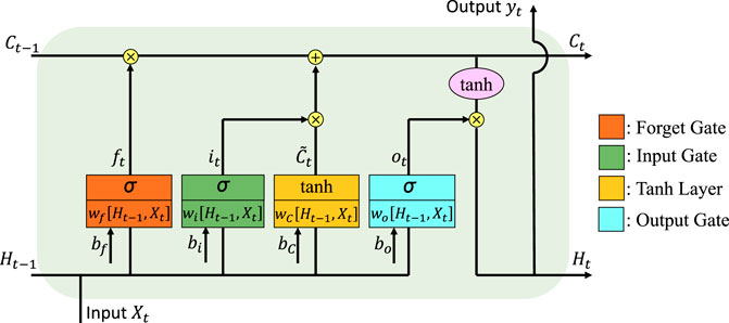
FIGURE 1. The long short-term memory unit.

and

${\mathit{H}}_{\mathit{t}}={\mathit{o}}_{\mathit{t}}\times \mathit{tanh}\left({\mathit{C}}_{\mathit{t}}\right)(6)$

The forget gate took the current time step input ($X_t$) and the hidden state ($H_{t-1}$) from the previous time step as concatenated input, multiplied the forget gate weight ($w_f$), added the forget gate bias ($b_f$), and applied the activation function. The input gate was provided with a concatenated input ($H_{t-1}$, $X_t$) with its weights ($w_i$) and biases ($b_i$) along with the candidate cell state ($C_t$). The cell state was updated with the forget gate ($f_t$) by applying both the previous cell state ($C_{t-1}$) additional to the input gate ($i_t$) and the candidate cell state (${\tilde{C}}_t$). The input gate determined whether or not the information in the current time step was memorized and stored in the cell state. The output gate ($o_t$) managed the output to update the cell state with its specific weights ($w_o$) and biases ($b_o$) using concatenated input similar to that of the input gate.

2.2 Design of the Input and Output of the Long Short-Term Memory Model

Before we introduce the neural network architecture, the design of the input and output of the proposed LSTM model is explained in this section. The goal of the proposed LSTM approach was to predict the PGA of the coming earthquake, as soon as possible after the arrival of the P wave, based on the measured seismic waves. Note that actually the problem is a regression one. However, in order to observe the intermediate prediction results more clearly, the target output of the LSTM model, shown in Figure 2, was designated as a step function with the amplitude of the PGA of the whole time history of the earthquake:

$\mathit{h}\left(\mathit{t}\right)=\{\begin{array}{c}0 , {\mathit{t}}_{\mathit{i}} \le \mathit{t} < {\mathit{t}}_{\mathit{p}}\\ \mathit{PGA} , {\mathit{t}}_{\mathit{p}} \le \mathit{t} \le {\mathit{t}}_{\mathit{e}}\end{array}(7)$

${\mathit{t}}_{\mathit{e}}={\mathit{t}}_{\mathit{p}}+{\mathit{t}}_{\mathit{w}}; {\mathit{t}}_{\mathit{w}}=0.5,1.0,1.5,2.0,2.5,3.0(8)$

FIGURE 2

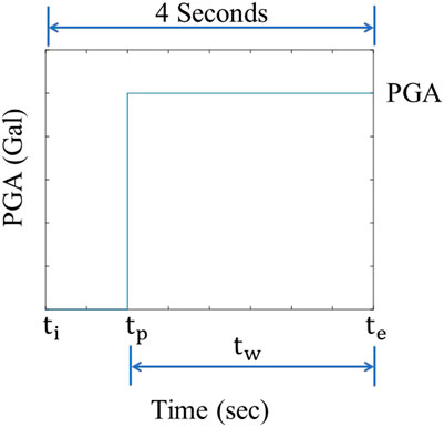
FIGURE 2. The schematic diagram of the target output of the LSTM model. $t_p$ is the P-wave arrival time; $t_i$ and $t_e$ are start time and end time, respectively; and $t_w$ is the length of the time-window between $t_p$ and $t_e$.

and

${\mathit{t}}_{\mathit{i}}=4-{\mathit{t}}_{\mathit{w}}(9)$

where $t_p$ was the P-wave arrival time determined based on the short-term average over long-term average (STA/LTA) algorithm; $t_i$ and $t_e$ were start time and end time, respectively; and $t_w$ was the length of the time-window between $t_p$ and $t_e$. As a result, the output was anticipated to be like a step function, but the predicted output was actually a series of predicted PGA values. Typical example of the output will be illustrated and discussed more in Section 3.3. Note that $t_p$ was approximately 2 s after the real first arrival time of the seismic wave. The total estimation time of the proposed algorithm to issue an alert consists of 1) the time between the P-wave arrival time and the trigger time determined by the STA/LTA algorithm, 2) the required length of $t_w$, and 3) the execution time of the proposed algorithm.

In this study, six $t_w$ lengths with an interval of 0.5 s were employed; hence, corresponding six truncated lengths with 4 s of “windowed” inputs were also employed. For instance, when $t_w=0.5$, only seismic waves with a time-window length of 0.5 s after the trigger were employed in the inputs, while those with a time-window length of 1.0 s after the trigger were employed when $t_w=1.0$, and so on. An example of the input and output targets of one typical earthquake is shown in Figure 3. The windowed input when $t_w=0.5$ is illustrated in Figure 3A. If the waveform is divided into windows with a smaller interval, then the alert could be issued once the predicted PGA values in any of the windows reach the threshold. Actually, the original design of the proposed algorithm is to predict the target PGA values at every time windows with an interval of 0.02 s. However, the program seems to have a problem dealing with the huge data with an interval of 0.02 s. A preliminary study was performed to determine whether the acceleration, velocity, and displacement time histories were used as the input of the proposed LSTM model. It was found that the performance of using both the acceleration and velocity was better than only using the acceleration or velocity, and including the displacement time history didn’t help. Hence both the acceleration and velocity are employed as the input in this study. Figures 3A–C show three acceleration time histories and three velocity time histories for different time-window lengths of the input. The velocity time histories were obtained from integration of the acceleration time histories. The corresponding target output time histories are shown in Figures 3D–F.

FIGURE 3

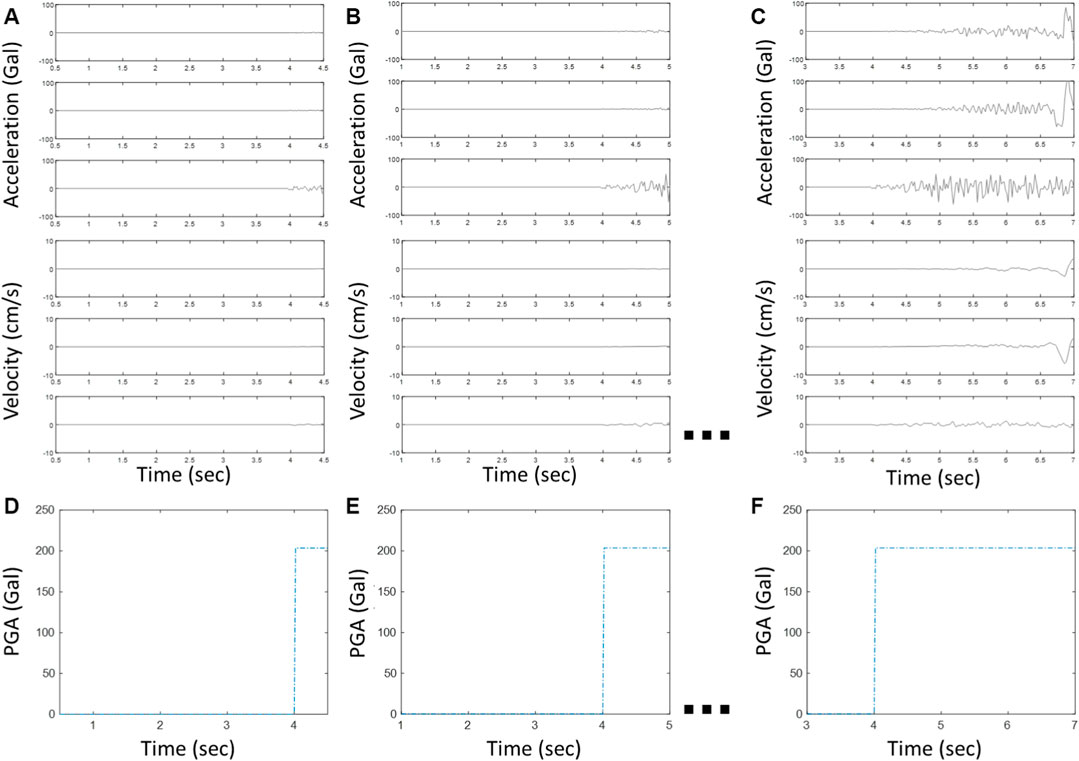
FIGURE 3. A typical example of the input/output of the LSTM model. (A) input of t_w = 0.5 s; (B) input of t_w = 1.0 s; (C) input of t_w = 3.0 s; (D) target output of t_w = 0.5 s; (E) target output of t_w = 1.0 s; and (F) target output of t_w = 3.0 s.

To save computational effort, the sampling rate of the input and output was reduced. Since the energy of seismic waves tended to be below 25 Hz, the original seismic waves were down-sampled from 200 to 50 Hz using an 8th order Chebyshev Type I infinite impulse response lowpass filter with a cutoff frequency of 40 Hz. The dimensions of the input and output of the LSTM model were 201 × 6 and 201 × 1, respectively. Hence, the window length of the input with 201 samples was 201 s × 0.02 s = 4.02 s. Both the input and output data were normalized using the RobustScaler normalization algorithm which removed the median and scaled the input and output data according to their interquartile range. Note that if longer or shorter waveform is used as the input or the sampling rate is changed, then the dimension of the input should be changed and the LSTM model should be modified and trained again.

2.3 Proposed Long Short-Term Memory Architecture

Because a previous study showed that the results of PGA prediction or large earthquake detection using conventional LSTM architecture were not acceptable (Wang et al., 2020), a dense LSTM architecture was employed in this study for PGA prediction. The dense LSTM architecture contained several LSTM layers, with each layer consisting of a parallel LSTM series, as shown in Figure 4. After the final dense LSTM layer, two fully connected layers were employed to generate the output data. The first layer consisted of a parallel ReLU (Rectified Linear Unit) series, which was a series of ReLU activation functions, while the second layer was a series of linear activation functions. The final LSTM model is shown in Figure 4. The number of LSTM layers and the number of parallel ReLU series in the first fully connected layer were determined based on a grid-search approach. The first hyper-parameter in the grid search was the number of LSTM layers, $N$, and the number of LSTM series in each layer was determined automatically as 2^N+2 in descending order. The number of LSTM layers considered in this study were (4, 5, 6). The other hyper-parameter in the grid search was the number of ReLU series in the first fully connected layer. The number of ReLU series in the first fully connected layer considered in this study were (8, 16, 32).

FIGURE 4

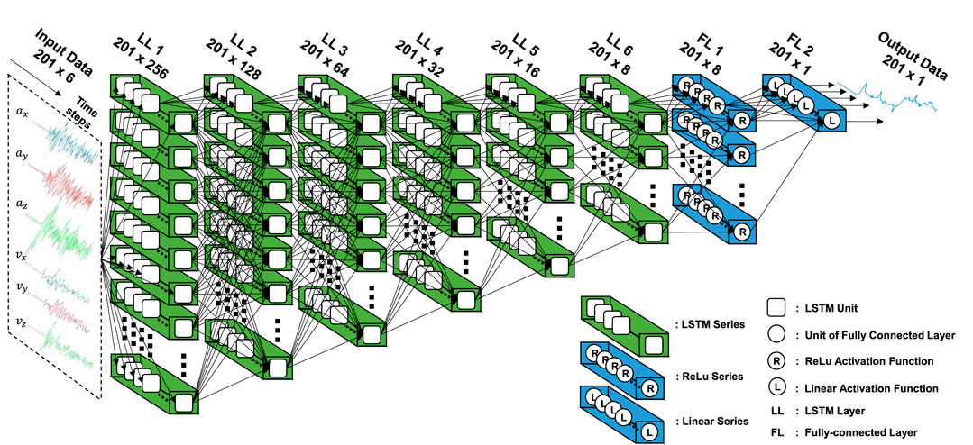
FIGURE 4. Proposed architecture of the LSTM model. LL 1 is the 1st LSTM Layer; LL 2 is the 2nd LSTM Layer and so on; FL 1 is the 1st Fully-connected Layer; FL 2 is the 2nd Fully-connected Layer.

2.4 Earthquake Data Sets

The Central Weather Bureau (CWB) of Taiwan collects high-quality data on ground motions at several hundred seismic stations around Taiwan via the Taiwan strong motion instrument program (TSMIP). The TSMIP data set of 91,128 earthquakes during the period from 29 July 1992, to 31 December 2006, was employed in this study. Approximately half of the TSMIP data, 40,000 earthquakes in total, for each PGA range defined by the CWB was used for training (32,000 earthquakes) and validation (8,000 earthquakes) of the proposed LSTM model, as listed in Table 1. The P-wave arrival time was determined based on the STA/LTA algorithm. In addition, two data sets of the most damaging recent earthquake events in Taiwan, i.e., the 2016 Meinong (Tainan) earthquake event and the 2018 Hualien earthquake event (https://www.worlddata.info), were employed to test the performance of the proposed LSTM approach.

TABLE 1

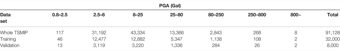
TABLE 1. The number of earthquakes of different ranges in the TSMIP data set.

2.5 Classification Metrics and Lead Time

In this study, the PGA threshold for general application was assumed to be 25 Gal. Once anyone of the values within the predicted PGA time history of a time-window length $t_w$ is equal to or larger than the threshold, the alert will be issued. In the field of machine learning, the confusion matrix of false positives (FPs), false negatives (FNs), true positives (TPs), and true negatives (TNs) allows performance to be easily visualized, as shown in Figure 5A. Note that the target of the LSTM prediction model is the PGA values, hence the problem is a regression one. But the application of the problem is actually if the alert is issued correctly, hence the precision, recall, and F1-score are calculated to estimate the performance of alert issuing of the proposed approach. The lead time, $t_{lead}$, is defined as the time of issuing an alert, $t_{alert}$, minus the time when the observed PGA reaches the threshold, $t_{PGA}$. That is, $t_{lead}=t_{alert}-t_{PGA}$. Note that if a correct alert is issued after the observed PGA reaches the threshold, i.e., negative lead time, it will be classified as an FN. The classification metrics of precision, recall, and F1 score are calculated as

$\mathit{\text{precision}}=\frac{\mathit{\text{TP}}}{\mathit{\text{TP}}+\mathit{\text{FP}}}(10)$

$\mathit{\text{recall}}=\frac{\mathit{\text{TP}}}{\mathit{\text{TP}}+\mathit{\text{FN}}}(11)$

FIGURE 5

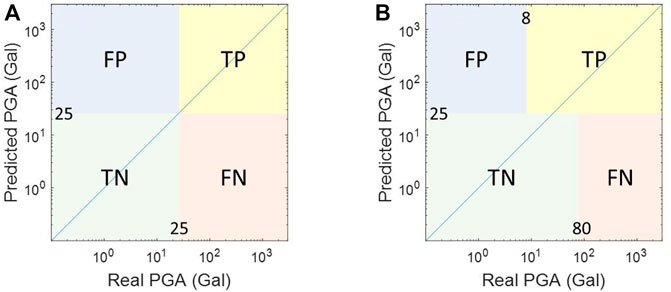
FIGURE 5. The confusion matrix when the threshold is designated as 25 Gal (A) without tolerance, and (B) with tolerance. FP is false positive; FN is false negative; TP is true positive; and TN is true negative.

and

$\mathit{\text{F}}\mathbf{1} \mathit{\text{score}}=\frac{\mathbf{2}\times \mathit{\text{precision}}\times \mathit{\text{recall}}}{\left(\mathit{\text{precision}}+\mathit{\text{recall}}\right)}(12)$

For community earthquake early warning, the false alert ratio (FAR) and missed alert ratio (MAR) are more straightforward to observe than alert performance, and can be calculated as

$\mathit{\text{FAR}}=\frac{\mathit{\text{FP}}}{\mathit{\text{TP}}+\mathit{\text{FP}}}(13)$

and

$\mathit{\text{MAR}}=\frac{\mathit{\text{FN}}}{\mathit{\text{TP}}+\mathit{\text{FN}}}(14)$

Note that the problem is a regression problem, hence the predict error is estimated using the root mean squared logarithmic error (RMSLE) value of the maximum predicted PGA, which will be explained in the next section.

3 Results and Discussion

3.1 Training and Validation

When large deviations exist in the data, e.g., the PGA of large earthquakes can be almost 1,000 times those of small ones, the RMSLE is often employed to estimate the loss in prediction accuracy, which is defined as

$\mathit{E}=\sqrt{\frac{\mathbf{1}}{\mathit{N}}{\displaystyle \sum }_{\mathit{j}=\mathbf{1}}^{\mathit{N}}{\left(\mathit{log}\left({\mathit{y}}_{\mathit{j}}^{\mathit{p}}+\mathbf{1}\right)-\mathit{log}\left({\mathit{y}}_{\mathit{j}}^{\mathit{r}}+\mathbf{1}\right)\right)}^{\mathbf{2}}}(15)$

where $y_j^r$ and $y_j^p$ are the actual and predicted PGA of the jth earthquake, respectively, and $N$ is the total number of earthquakes. The parameters in the LSTM model were updated based on the Nadam optimizer with a learning rate = 0.0001 and batch size = 32 during the training process. The training process stopped when validation loss kept increasing over three successive epochs; the loss history during a typical training process of the LSTM is shown in Figure 6. The LSTM model was trained using Python language on an Intel^® Core™ i7-6700 CPU 3.40 GHz computer.

FIGURE 6

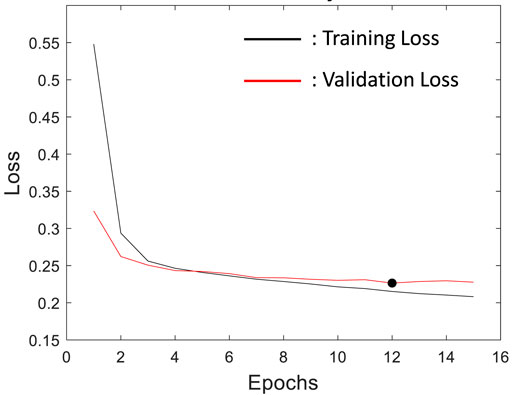
FIGURE 6. Loss history during a typical training process.

3.2 Grid Search Results

In this study, a grid search approach was employed to determine the two hyper-parameters (the number of LSTM layers and the number of ReLU series in the first fully connected layer) in the LSTM architecture. Both PGA prediction accuracy and lead-time length were considered in the evaluation of the performance of the LSTM architecture. Specifically, the model score, $S_M$, of the LSTM architecture was calculated using the Min-Max normalized F1 score, ${\tilde{F}}_1$, and the Min-Max normalized average lead-time, ${\tilde{t}}_{lead}$, (without tolerance) as

${\mathit{S}}_{\mathit{M}}=\mathit{ }{\tilde{\mathit{F}}}_1+{\tilde{\mathit{t}}}_{\mathit{lead}}(16)$

Table 2 shows the F1 score, average lead time, and model score of the nine combinations of the two hyper-parameters. The highest model score was achieved by the 7th LSTM model. Thus, the selected LSTM model consisted of six hidden LSTM layers and eight ReLU series in the first fully connected layer, which was used in the following analyses.

TABLE 2

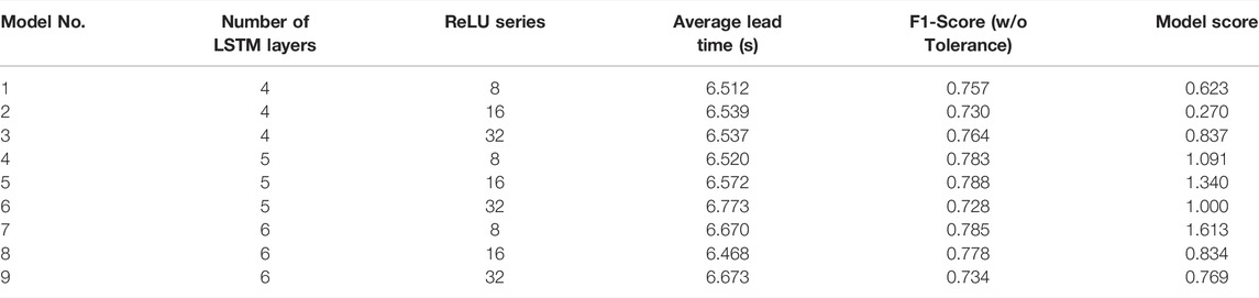
TABLE 2. The nine combinations of the two hyper-parameters of the LSTM models. The F1 score, average lead time, and model score of these models are also given.

3.3 Typical Predicted Peak Ground Acceleration Time Histories

In this section, the raw output of the predicted PGA time history using the proposed LSTM approach is discussed. The predicted PGA time histories of a TP case using different input windows are shown in Figure 7. When t_w = 0.5 s, the observed PGA time history and the predicted PGA time history of the LSTM model are shown as the thin dashed–dotted gray line and the thick color line, respectively, in Figure 7A. The observed PGA time history is a series of the peak ground acceleration observed till different time. The target PGA is shown as the step function in a brown dashed–dotted line style, where the trigger time is indicated by the location of a “jump” in the step function. Because the predicted PGA exceeds 25 Gal at approximately 4.04 s (shown as the dotted salmon-colored vertical line), the alert is issued in this window, i.e., at 4.5 s, as indicated by the dashed–dotted, teal-colored vertical line (at the very end of this figure). When t_w = 1.0 s (Figure 7B), since the predicted PGA already exceeded the threshold in the previous window when t_w = 0.5 s, the alert has already been issued and the alert time remains at 4.5 s. The measured accelerations exceed the threshold approximately at 4.88 s (shown as the dashed purple line); hence, the lead time of this TP case is 4.88 − 4.5 = 0.38 s. Note that an alert is classified as a TP only when it is issued before the threshold is reached, i.e., the lead time is positive. If a correct alert is issued but the lead time is zero or negative, the alert is classified as a false negative (FN). The observed PGA time history and the predicted PGA time history of the LSTM model when t_w = 1.5, 2.0, 2.5, and 3.0 s are shown in Figures 7C–F. Figures 7A–F can be combined together to produce Figure 8A for conciseness of this paper. In summary, the maximum amplitude of the predicted PGA time history (in short, maximum predicted PGA) at each window when t_w = 0.5, 1.0, 1.5, 2.0, 2.5, and 3.0 s is 42.5, 51.2, 88.6, 67.8, 79.5, and 115.2 Gal, respectively. Although the target is a step function, the predicted output is approximately a monotonically-increasing step-like PGA time history. This phenomenon is also observed in Otake et al. (2020). Although the seismic intensity of an earthquake has only one value determined by the largest intensity during the earthquake, the predicted output of Otake et al. (2020) is a series of seismic intensity predicted at different time.

FIGURE 7

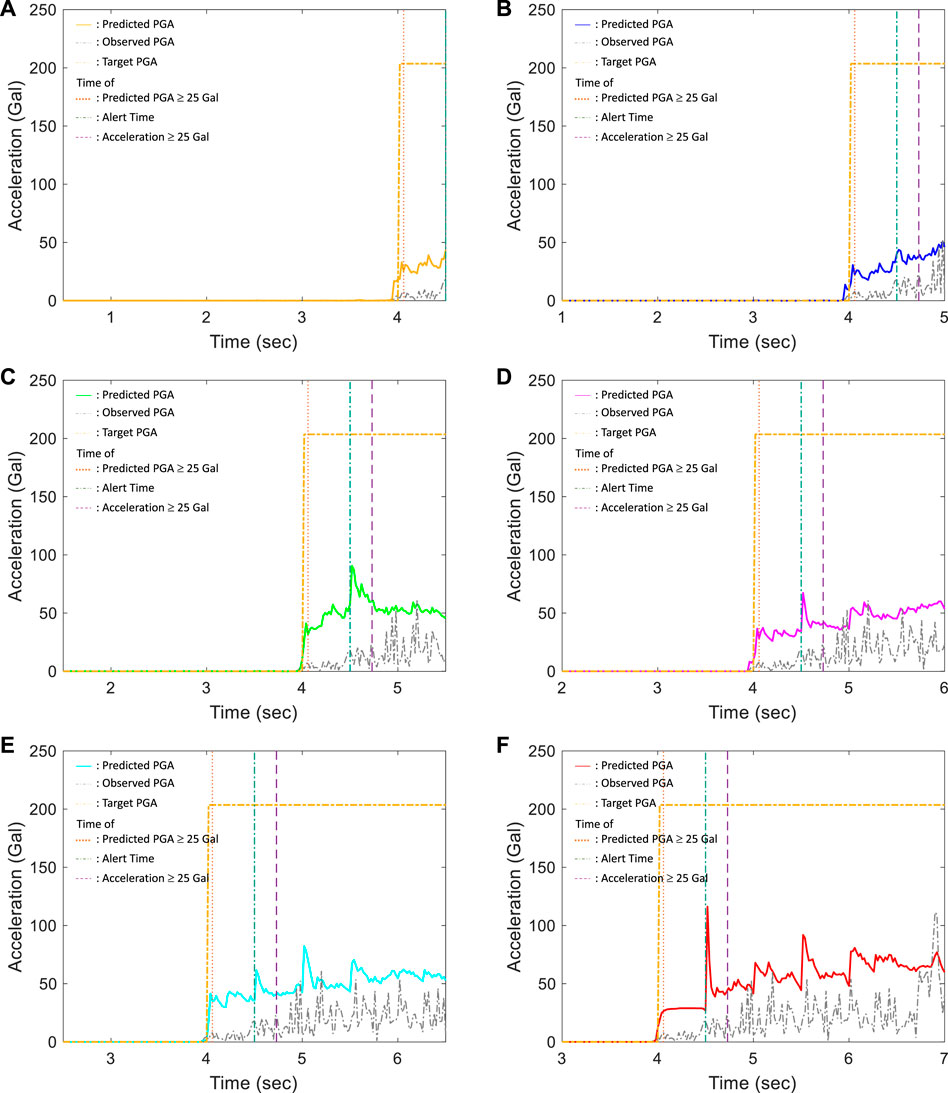
FIGURE 7. The observed PGA time histories, predicted PGA time histories, and target PGA time histories of a typical true positive (TP) case using (A) t_w = 0.5 s; (B) t_w = 1.0 s; (C) t_w = 1.5 s; (D) t_w = 2.0 s; (E) t_w = 2.5 s; and (F) t_w = 3.0 s.

FIGURE 8

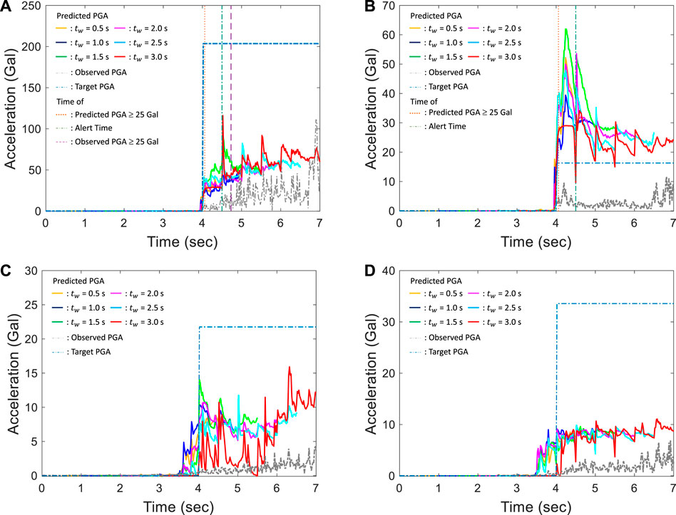
FIGURE 8. Observed PGA time histories, predicted PGA time histories of different windows, and target PGA time histories of a typical (A) TP, (B) FP, (C) TN, and (D) FN case.

The results of a typical FP case using different input windows are shown in Figure 8B. Because the predicted PGA exceeds 25 Gal at approximately 4.02 s (shown as the dotted salmon-colored vertical line), the alert is issued in this window, i.e., at 4.5 s (shown as the dashed–dotted, teal-colored vertical line). The maximum predicted PGA value at each window when t_w = 0.5, 1.0, 1.5, 2.0, 2.5, and 3.0 s is 52.1, 39.9, 62.2, 53.5, 48.6, and 33.7 Gal, respectively. However, the actual PGA is only about 16 Gal, as indicated by the dashed–dotted cobalt blue step function of the target PGA; hence, this is an FP case if no tolerance of the error of the predicted PGA is allowed. The results of a typical true negative (TN) case using different input windows are shown in Figure 8C. Although the time histories of the predicted PGA at each window are quite different, the maximum predicted PGA of all windows are approximately below 16 Gal, hence no alert will be issued in this case. The actual PGA is only about 21.7 Gal as indicated by the step function of the target PGA; hence, no alert is necessary in this case. The results of a typical FN case using different input windows are shown in Figure 8D. The actual PGA is approximately 33.6 Gal as indicated by the step function of the target PGA. However, the maximum predicted PGA of all the six windows is only about 11.1 Gal; hence, no alert is issued in this case. Note that because the P-wave arrival time is determined automatically using the STA/LTA algorithm, it could be after the real arrival of the P-wave for approximately 2 s, especially for the small earthquakes. As a result, for the small earthquakes, small acceleration signals already exist before the P-arrival time picked by the STA/LTA algorithm. Hence PGAs of approximately 5 Gal in Figures 8C,D could be predicted before the P-wave arrival times.

3.4 General Performance of the Taiwan Strong Motion Instrument Program Data Set

The accuracy of the predicted PGA of the entire TSMIP data set of 91,119 earthquakes is discussed here to understand the general performance of the LSTM model in PGA prediction. The predicted PGA is a time history of each window, hence the data set for predicting the PGA of 91,119 earthquakes using six different windows is quite substantial. Because an alert will be issued when any predicted PGA within any window reaches the threshold, the maximum predicted PGA within all the windows is a critical value affecting performance in issuing alerts and will be discussed here. Figure 9 illustrates the comparison between the maximum predicted PGA and the actual PGA of all 91,119 earthquakes. The RMSLE value of the maximum predicted PGA is 0.804. Besides, the standard deviation error (STD) of the maximum predicted PGA is 0.563, while the mean absolute error percentage (MAPE) of the maximum predicted PGA is 131.0%. The large value of MAPE is because there are many earthquakes of small PGA. It is evident that the maximum predicted PGA tends to be larger than the actual one, which is reasonable because the maximum value of the predicted PGA time history within all the windows is considered. For example, the maximum predicted PGA in the typical FP case in Figure 8B is approximately 62 Gal, which is the largest predicted value when t_w = 1.5 s, while the actual PGA is approximately 11 Gal.

FIGURE 9

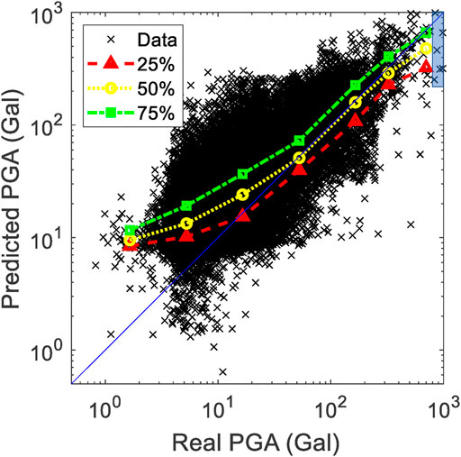
FIGURE 9. Comparison between the predicted PGA and actual PGA of the entire TSMIP data set using the proposed LSTM approach. The distribution of the earthquakes with real PGA larger than 800 Gal is marked with the blue box.

If the magnitude and location of the earthquakes were perfectly estimated right after the arrival of the P wave, the PGA could be predicted base on the ground motion prediction equation (GMPE), which is used in many EEW systems in the world. Based on the GMPE developed by Jean et al. (2006), the RMSLE of the predicted PGA is 1.102, which is much larger than the one using the proposed LSTM approach. Hence although the deviation in Figure 9 looks quite large, the calculated RMSLE is still quite acceptable.

The performance of the alerts issued based on the PGA prediction results of the LSTM model is discussed next. The confusion matrix of FP, FN, TP, and TN when no tolerance of the predicted PGA is allowed and the PGA threshold for issuing an alert is designated as 25 Gal (Figure 5A). The performance metrics based on the confusion matrix, such as the number of TPs, FPs, FNs, TNs, and the values of the F1 score, precision, and recall are shown in Table 3. Although recall is quite high (95.17%), precision and F1 score are quite low, only 32.4% and 48.3%, respectively. This is because the predicted PGA tends to be overestimated, hence the number of FPs is quite large, i.e., 32,720, compared to the number of TPs, i.e., 15,684. In other words, the false alert ratio (FAR), at 67.6%, is quite high and the missed alert ratio (MAR), at 4.90%, is quite low.

TABLE 3

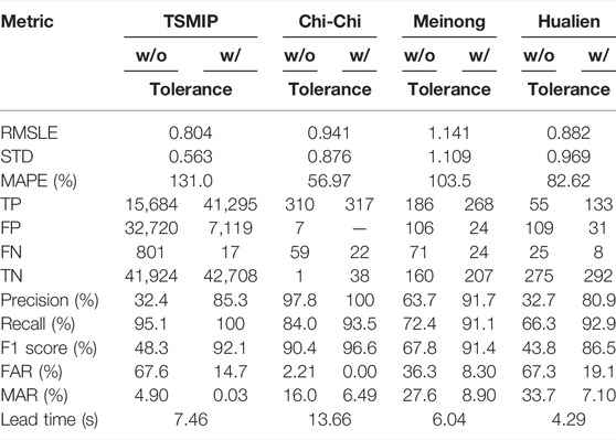
TABLE 3. The performance metrics of the TSMIP, Chi-Chi earthquake, Meinong earthquake, and Hualien earthquake data sets using the proposed LSTM model.

In practical, a tolerance of ±1 level of intensity prediction is accepted and employed in the Japan Meteorological Agency, Japan (JMA, 2016) and the CWB, Taiwan. They define the intensity prediction accuracy ratio as the ratio of the predicted intensity scale located within a one-scale difference from the real intensity scale among all the considered earthquake data. In this study, the tolerance range proposed by Meier (2017) is employed when evaluating the classification performance of an EEW system. The ±1 level of the CWB intensity scale based on PGA is shown in Figure 5B, and the performance metrics of tolerance are also summarized in Table 3. While tolerance is allowed, only 17 and 7,119 cases of FNs and FPs, respectively, remain and precision, recall, and F1-score increase to 85.3%, 100.0%, and 92.1%, respectively. Hence, the overall potential alert performance using the proposed LSTM model appears to be quite promising in general if tolerance is allowed. The false alert ratio (FAR), at only 14.7%, is quite acceptable, and the missed alert ratio (MAR), at 0.03%, is almost zero.

The distribution of lead times of the cases when both the actual and predicted PGA is ≥25 Gal is shown in Figure 10. The lead times of these cases are between −1 and 26 s, and the average lead time is 7.46 s. The lead times of only five cases are negative, and these cases are classified as FN, as shown in Figure 10B.

FIGURE 10

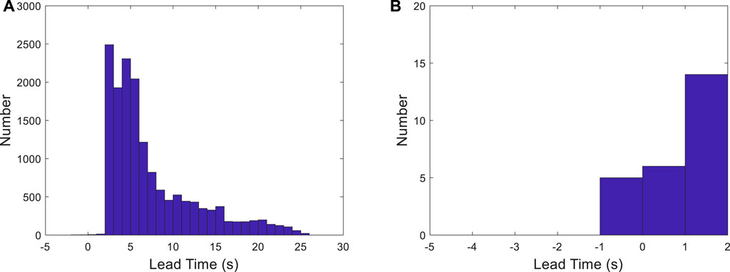
FIGURE 10. (A) Lead time distribution of the TSMIP data set; and (B) close view of the distribution of lead times shorter than 2 s.

3.5 Performance of the Chi-Chi Earthquake Data Set

The Chi-Chi earthquake data set is also included in the TSMIP data set of 91,119 earthquakes, hence approximately half of the data of the Chi-Chi earthquake are in the training dataset and validation dataset. The fault rupture of the Chi-Chi earthquake has been reported as long and complex (Ma et al., 2001). In addition, several studies have indicated that the magnitude or intensity estimation based on the short beginning of vibration signals (usually several seconds) is not reliable for such large earthquakes, which are usually generated by a long and complex rupture (e.g., Wu and Zhao, 2006; Rydelek et al., 2007; Hoshiba and Iwakiri, 2011; Kodera, 2019). As in the case of the Chi-Chi earthquake, underestimation of PGA is usually observed when the prediction model is established using SVR (Hsu et al., 2013), a multilayer feedforward network (Hsu et al., 2020), or a CNN (Hsu et al., 2021). Hence, we also assessed the PGA prediction results of the Chi-Chi earthquake data set using the proposed LSTM approach in this study, as shown in Figure 11A and Table 3. The maximum PGA of the same windows, i.e., 0.5, 1, 1.5, 2, 2.5, and 3 s, after the trigger, predicted using the SVR approach (Hsu et al., 2013) and the CNN approach (Hsu et al., 2021), is shown in Figures 11B,C for comparison, respectively. It is evident that the PGA predicted using the SVR approach and the CNN approach is substantially underestimated, while that predicted using the LSTM approach is much closer to the actual PGA, although the predicted PGA of some earthquakes is still underestimated. The number of TPs, FPs, FNs, TNs, and the RMSLE, STD, MAPE, F1 score, precision, recall, FAR, and MAR using the SVR approach and the CNN approach are shown in Table 4. Tables 3, 4 show that while the FARs of the LSTM, SVR, and CNN approaches are very low, the MARs of the latter two approaches are much higher than those of the former. In addition, the average lead time of the proposed LSTM approach is much longer than that of the SVR and CNN approaches. Based on these results, the proposed LSTM approach may have an advantage over the other approach in more accurately predicting the PGA of earthquakes with a long and complex rupture process, but further study is necessary to support this finding.

FIGURE 11

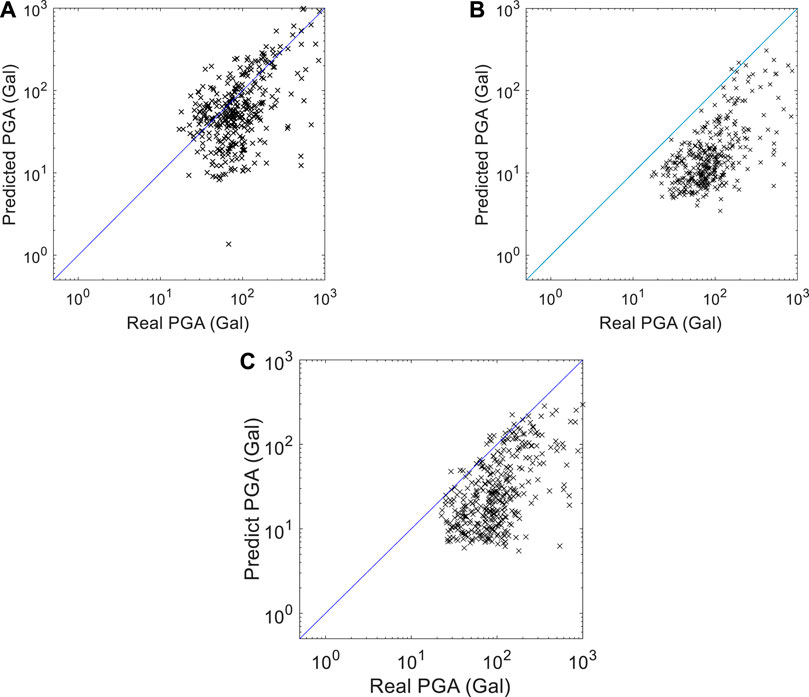
FIGURE 11. Comparison between the predicted PGA and actual PGA of the Chi-Chi data set using (A) the proposed LSTM approach, (B) the SVR approach, and (C) the CNN approach.

TABLE 4

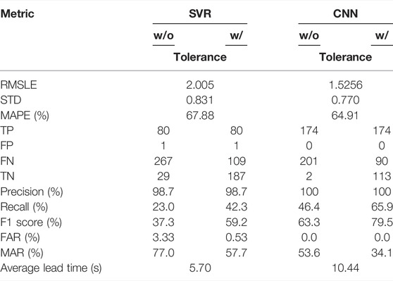
TABLE 4. The performance metrics of the Chi-Chi earthquake data set using the SVR approach and the CNN approach.

3.6 Performance of the Independent Data Sets

In addition to the TSMIP data set, the performance of the proposed LSTM approach was also studied using the independent data sets of the 2016 Meinong earthquakes and the 2018 Hualien earthquakes. The comparison between the predicted and actual PGA of these two data sets is shown in Figure 12. The distribution indicates that the independent data sets could also demonstrate the anticipated accuracy of PGA prediction. The RMSLE of the Meinong and Hualien data sets was 1.410 and 0.882, respectively. The performance metrics, based on the confusion matrices in Figure 5, are shown in Table 3. If no tolerance is allowed, the number of FPs is larger than the number of FNs, resulting in higher recall than precision of both data sets. If tolerance is allowed, precision, recall, and F1 score of these two data sets are quite high, between 80.9% and −92.9%. Hence, the performance of alert classification seems quite promising in general if tolerance is allowed.

FIGURE 12

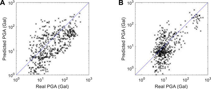
FIGURE 12. Comparison between the predicted PGA and actual PGA of the (A) Meinong data set, and (B) Hualien data set.

The lead times of these two data sets were between −2 and 17 s, and the average lead times were 6.04 and 4.29 s, as shown in Figure 13 and Table 3. Although the predicted PGA was larger than the threshold for all the cases with a negative lead time, these cases were classified as FN due to late alerts, whose locations are shown as inverted triangles in Figure 14. Note that it is not necessary for the stations with a negative lead time to be close to the epicenter. In fact, the lead time of only one of these cases was <−1; the observed PGA and the predicted PGA using different input windows of this case are shown in Figure 15A. The amplitude of observed PGA time history was quite small and increased very slowly with time, which may make accurate prediction of PGA in time quite difficult. In all other cases with negative lead times, their lead times were actually between −0.5 and 0 s. A typical case with negative lead times is shown in Figure 15B. Because the predicted PGA exceeded 25 Gal in the same time window with the actual PGA exceeding 25 Gal, the negative lead-time cases could become positive if smaller intervals are used (for example, when the time interval is changed to 0.1 s).

FIGURE 13

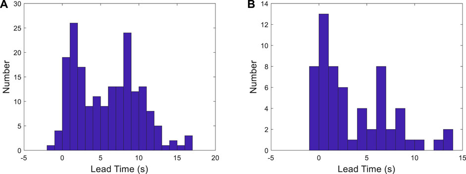
FIGURE 13. Lead time distribution of the (A) Meinong data set, and (B) Hualien data set.

FIGURE 14

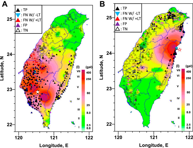
FIGURE 14. The locations of the stations of different classification conditions of the (A) Meinong data set, and (B) Hualien data set. The background indicates the distribution of observed PGA. LT is lead time, and the star marker is the epicenter.

FIGURE 15

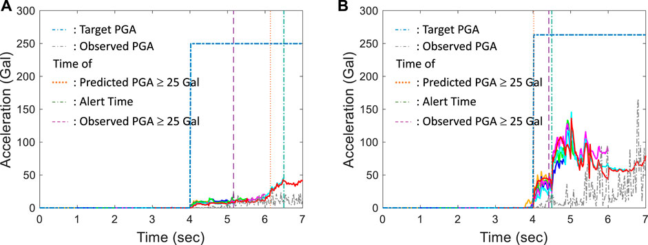
FIGURE 15. Observed PGA time histories, predicted PGA time histories of different windows, and target PGA time histories of (A) the only case of lead time < −1 s in the Meinong data set, and (B) a typical case of lead time < 0 s in the independent data sets.

The locations of the classification results with tolerance for the Meinong earthquakes are shown in Figure 14A. The background of PGA distribution may result from the northwestward rupture of the left–lateral strike-slip fault. Most of the alerts of the stations close to the epicenter are TP. In addition, most of the stations with FN alerts are located in the region approximately 80–130 km north of the epicenter. This phenomenon could mainly be related to the seismic wave difference due to the rupture directivity of the fault. In addition, most of the FP alerts are located in east Taiwan. Besides the rupture directivity of the fault, another possible reason for this phenomenon could be the effect of the path from west to east through the mountainous area in central Taiwan. In the case of the Hualien earthquakes, the background of PGA distribution in Figure 14B indicates that the rupture was oriented toward the south, which was identical to the focal mechanism solutions. The majority of the alerts of stations near the epicenter were TP, except for those of several stations very close to the epicenter. Most of the FP stations were located north of the epicenter. This phenomenon may also be related to the seismic wave difference due to the rupture directivity of the fault.

3.7 Discussion of the Alert Criterion

From the general performance of the LSTM approach to the analysis of the TSMIP data set, it is evident that the predicted PGA tends to be overestimated, resulting in a higher FAR. The alert is issued once the predicted PGA is equal to or larger than the threshold in any of the six windows. If the alert is issued only when the predicted PGA of two consecutive windows reaches the threshold, then the number of false alerts should be reduced. Hence, in this section, an alternative algorithm for issuing an alert is proposed to reduce the FAR. This algorithm has two conditions, and the alert will be issued when anyone of the conditions is fulfilled. The first is satisfied when the predicted PGA is equal to or larger than the threshold in two consecutive windows. The second is satisfied when the predicted PGA is equal to or larger than the threshold in the last window (t_w = 3.0 s). It is because there are no further windows after this one. As shown in Table 5, the number of FP cases decreased from 32,720 to 27,024, while the FAR decreased from 14.7% to 11.5% when tolerance was allowed. However, the number of FN cases increased from 17 to 20, while the MAR increased from 0.03% to 0.04% when tolerance was allowed, and the average lead time also decreased from 7.46 to 6.91 s. A trade-off was always present between FP cases and the FN cases, and also between prediction accuracy and lead time. If more missed alerts are not tolerable, then the original criterion to issue an alert should be employed.

TABLE 5

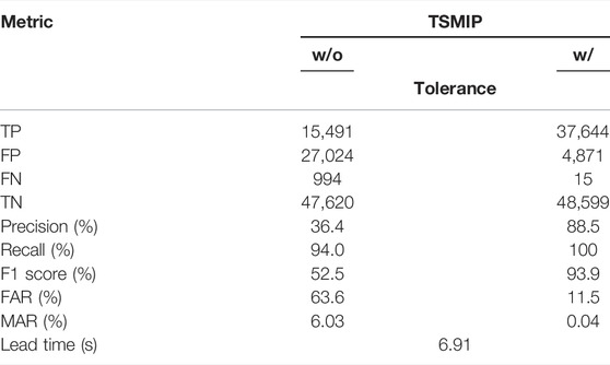
TABLE 5. The performance metrics of the TSMIP data set using the proposed LSTM model with an alternative alert criterion.

3.8 Performance of Different Peak Ground Acceleration Thresholds

As discussed in the Introduction, a threshold can be designated for different applications. In this study, two alternative thresholds were considered. The first was a relatively small threshold, which is required to issue a command to automatically park machines in semiconductor fabrication plants during the manufacturing process even when the intensity of the coming seismic vibration is small. By doing so, these machines can restart the manufacturing process after the earthquake much faster than when they are shut down by the emergency stop due to the measured vibration signals. The reduced time required to restart the manufacturing process is very beneficial to the semiconductor fabrication plants. Hence, the threshold of 8 Gal was considered in this study, and the general performance of the TSMIP data set was assessed.

The performance metrics when the PGA threshold for issuing an alert is designated as 8 Gal are shown in Table 6. If no tolerance is allowed, the number of FPs is quite large, i.e., 31,047, compared to the number of TPs, i.e., 59,778, resulting in the FAR being quite high at 34.2%. Note that the FAR is much lower than that (it is 67.6%) when the threshold is 25 Gal (Table 3). On the other hand, the number of FNs is only 41, resulting in the MAR being only 0.07%. The average lead time is 6.60 s. The number of FPs becomes only 112, which is very small compared to the number of TPs, i.e., 90,713, when a ±1 level of the CWB intensity scale is employed, as shown in Figure 16A. In addition, only three FNs remain. Hence the FAR and MAR are very small, i.e., 0.12% and 0.01%, respectively. As a result, the performance of alert classification using 8 Gal as the threshold seems quite promising in general if tolerance is allowed.

TABLE 6

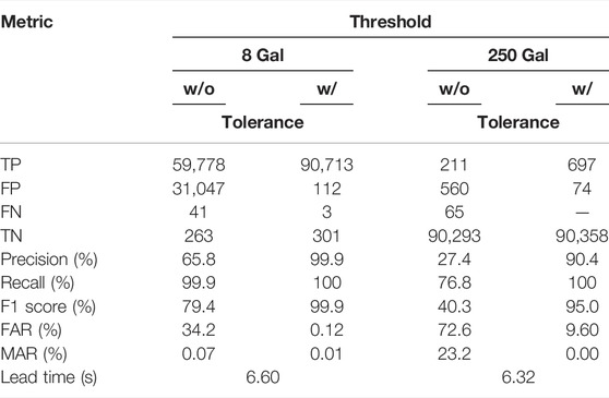
TABLE 6. The performance metrics of the TSMIP data set using the proposed LSTM model with different PGA thresholds.

FIGURE 16

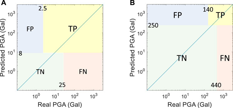
FIGURE 16. The confusion matrix with tolerance when the threshold is designated as (A) 8 Gal, and (B) 250 Gal.

The other threshold is relatively large, which could be useful for nuclear power plants because their design basis earthquake is much larger than that of ordinary structures. Hence, the threshold of 250 Gal is studied here, and the general performance of the TSMIP data set is assessed. The performance metrics when the PGA threshold for issuing an alert is designated as 250 Gal are also shown in Table 6. If no tolerance is allowed, the number of FPs is only 560, but it is relatively large compared to the number of TPs, i.e., 211, resulting in the FAR, at 72.6%, being quite high. On the other hand, the number of FNs is only 65, which is relatively small compared to the number of TPs, resulting in the MAR being only 23.2%. The average lead time is 6.32 s. When a ±1 level of the CWB intensity scale is employed here, as shown in Figure 16B, the number of FPs is only 74, which is very small compared to the number of TPs, i.e., 697. In addition, the number of FNs becomes 0. Hence, the FAR and MAR are very small, i.e., 9.60% and 0.00%, respectively, lower than 14.7% and 0.03% when the threshold is 25 Gal (Table 3). As a result, the performance of alert classification using 250 Gal as the threshold also seems quite acceptable in general if tolerance is allowed.

4 Conclusion

In this study, a dense architecture was proposed for the LSTM neural network to predict the PGA of the incoming seismic wave at the same site. The input data of the LSTM model were the acceleration and velocity time histories of different window lengths of P-wave data after the trigger. The general performance of the proposed LSTM model using the TSMIP data set with 91,128 earthquakes was quite acceptable. However, the predicted PGA of the proposed LSTM model tended to be overestimated, hence a higher FAR (14.7%) and a lower MAR (0.03%) were obtained when a ±1 level of the CWB intensity scale was tolerated, and the average lead time was 7.46 s for the whole TSMIP data set.

Surprisingly, the accuracy of the predicted PGA of the Chi-Chi earthquake using the proposed LSTM model was quite acceptable, resulting in a zero FAR (0.00%) and a low MAR (6.49%) when a ±1 level of the CWB intensity scale was tolerated. Note that the predicted PGA of the Chi-Chi earthquake in previous studies was always seriously underestimated. For comparison, if the maximum predicted PGA for the same windows after the trigger is considered using the SVR approach, an FAR of 0.53% and a high MAR value of 57.7% with a shorter average lead time of 5.70 s are obtained. This illustrates one of the merits of the proposed LSTM approach.

Two independent data sets for damaging earthquakes that occurred recently in Taiwan were employed to validate the proposed LSTM approach. The results indicate that the anticipated accuracy of PGA prediction could also be demonstrated with the independent data sets. When tolerance was allowed, the performance of alert classification appeared quite promising in general because precision, recall, and F1-score were quite high, i.e., between 80.9% and −92.9%. The lead times of these two data sets were between −2 and 17 s, and the average lead times were 6.04 and 4.29 s. Lead time can be improved if smaller intervals between time windows are employed, especially for the cases with negative lead times, but further studies are required to support this hypothesis.

Because the proposed LSTM approach tended to predict overestimated PGA in general, an alternative algorithm to issue alerts is proposed to reduce the FAR. In this alternative algorithm, an alert will be issued only if the PGA threshold is satisfied in two consecutive windows (except the last window). The performance of the alternative algorithm was tested with the TSMIP data set. When tolerance was allowed, although the FAR decreased from 14.7% to 11.5%, the MAR increased from 0.03% to 0.04% and the average lead time decreased from 7.46 to 6.91 s.

The threshold can be designated for different applications. In this study, two alternative thresholds were studied. The performance of the different thresholds was tested with the TSMIP data set. If the PGA threshold for issuing an alert was designated as 8 Gal and tolerance was allowed, the FAR and MAR were very small, i.e., 0.12% and 0.01%, respectively, and the average lead time became somewhat shorter, i.e., 6.60 s. If the PGA threshold for issuing an alert was designated as 250 Gal and tolerance was allowed, the FAR and MAR were also very small, i.e., 9.60% and 0.00%, respectively, and the average lead time also became a little shorter, i.e., 6.32 s. Note that these FAR and MAR values were smaller than those, i.e., 14.7% and 0.03%, when the threshold was 25 Gal. However, more studies are required because the number of earthquakes with a PGA of <2.5 Gal or >250 Gal is not large enough. Nevertheless, the results still indicate possible application of the proposed LSTM approach to different designated thresholds.

Data Availability Statement

Publicly available datasets were analyzed in this study. This data can be found here: The strong-motion accelerations of the Taiwan strong motion instrumentation program (TSMIP) can be downloaded from the geophysical database management system (GDMS) website (http://gdms.cwb.gov.tw/index.php, last accessed September 2021).

Author Contributions

TH designed the research study and wrote sections of the manuscript. AP constructed the LSTM and ran the analysis.

Conflict of Interest

The authors declare that the research was conducted in the absence of any commercial or financial relationships that could be construed as a potential conflict of interest.

Publisher’s Note

All claims expressed in this article are solely those of the authors and do not necessarily represent those of their affiliated organizations, or those of the publisher, the editors and the reviewers. Any product that may be evaluated in this article, or claim that may be made by its manufacturer, is not guaranteed or endorsed by the publisher.

Acknowledgments

The authors want to thank Dr. Hung-Yi Lee, the professor of the Department of Computer Science and Information Engineering at National Taiwan University, Taiwan, for his generous support of this research. The authors also want to thank the Taiwan Strong Motion Instrument Program operated by Central Weather Bureau (CWB) in Taiwan for providing high-quality strong ground motions caused by earthquakes around Taiwan. The strong-motion accelerations of the Taiwan strong motion instrumentation program (TSMIP) can be downloaded from the geophysical database management system (GDMS) website (http://gdms.cwb.gov.tw/index.php, last accessed September 2021).

References

Allen, R. M., and Melgar, D. (2019). Earthquake Early Warning: Advances, Scientific Challenges, and Societal Needs. Annu. Rev. Earth Planet. Sci. 47, 361–388. doi:10.1146/annurev-earth-053018-060457

CrossRef Full Text | Google Scholar

Böse, M., Heaton, T., and Hauksson, E. (2012). Rapid Estimation of Earthquake Source and Ground-Motion Parameters for Earthquake Early Warning Using Data from a Single Three-Component Broadband or Strong-Motion Sensor. Bull. Seismol. Soc. Am. 102 (2), 738–750.

Google Scholar

Chiang, Y.-J., Chin, T.-L., and Chen, D.-Y. (2022). Neural Network-Based Strong Motion Prediction for On-Site Earthquake Early Warning. Sensors 22, 704. doi:10.3390/s22030704

PubMed Abstract | CrossRef Full Text | Google Scholar

Cremen, G., and Galasso, C. (2020). Earthquake Early Warning: Recent Advances and Perspectives. Earth-Science Rev. 205 (February), 103184. doi:10.1016/j.earscirev.2020.103184

CrossRef Full Text | Google Scholar

Cuéllar, A., Espinosa-Aranda, J. M., Suarez, R., Ibarrola, G., and Uribe, A. (2014). “The Mexican Seismic Alert System (SASMEX): its Alert Signals, Broadcast Results and Performance during the M 7.4 Punta Maldonado Earthquake of March 20th, 2012,” in Early Warning for Geological Disasters. Editors F. Wenzel, and Z. Zschau (Berlin: Springer-Verlag), 71–87.

Google Scholar

Fayaz, J., and Galasso, C. (2022). A Deep Neural Network Framework for Real-Time On-Site Estimation of Acceleration Response Spectra of Seismic Ground Motions. Computer-Aided Civ. Infrastructure Eng., 1–17.

Google Scholar

Fujinawa, Y., and Noda, Y. (2013). Japan’s Earthquake Early Warning System on 11 March 2011: Performance, Shortcomings, and Changes. Earthq. Spectra 29 (S1), S341–S368. doi:10.1193/1.4000127

CrossRef Full Text | Google Scholar

Hochreiter, S., and Schmidhuber, J. (1997). Long Short-Term Memory. Neural Comput. 9 (8), 1735–1780. doi:10.1162/neco.1997.9.8.1735

PubMed Abstract | CrossRef Full Text | Google Scholar

Hoshiba, M., and Iwakiri, K. (2011). Initial 30 Seconds of the 2011 off the Pacific Coast of Tohoku Earthquake (M W 9.0)-amplitude and τ C for Magnitude Estimation for Earthquake Early Warning-. Earth Planet Sp. 63, 553–557. doi:10.5047/eps.2011.06.015

CrossRef Full Text | Google Scholar

Hsu, T.-Y., and Huang, C.-W. (2021). Onsite Early Prediction of PGA Using CNN with Multi-Scale and Multi-Domain P-Waves as Input. Front. Earth Sci. 9, 626908. doi:10.3389/feart.2021.626908

CrossRef Full Text | Google Scholar

Hsu, T.-Y., Huang, S.-K., Chang, Y.-W., Kuo, C.-H., Lin, C.-M., Chang, T.-M., et al. (2013). Rapid On-Site Peak Ground Acceleration Estimation Based on Support Vector Regression and P-Wave Features in Taiwan. Soil Dyn. Earthq. Eng. 49, 210–217. doi:10.1016/j.soildyn.2013.03.001

CrossRef Full Text | Google Scholar

Hsu, T.-Y., Kuo, C.-H., Wang, H.-H., Chang, Y.-W., Lin, P.-Y., and Wen, K.-L. (2021). The Realization of an Earthquake Early Warning System for Schools and its Performance during the 2019 ML 6.3 Hualien (Taiwan) Earthquake. Seismol. Res. Lett. 92 (1), 342–351. doi:10.1785/0220190329

CrossRef Full Text | Google Scholar

Hsu, T.-Y., Wang, H.-H., Lin, P.-Y., Lin, C.-M., Kuo, C.-H., and Wen, K.-L. (2016). Performance of the NCREE's On-Site Warning System during the 5 February 2016Mw6.53 Meinong Earthquake. Geophys. Res. Lett. 43, 8954–8959. doi:10.1002/2016gl069372

CrossRef Full Text | Google Scholar

Hsu, T.-Y., Wu, R.-T., Liang, C.-W., Kuo, C.-H., and Lin, C.-M. (2020). Peak Ground Acceleration Estimation Using P-Wave Parameters and Horizontal-To-Vertical Spectral Ratios. Terr. Atmos. Ocean. Sci. 31 (1), 1–8. doi:10.3319/tao.2019.07.04.01

CrossRef Full Text | Google Scholar

Hsu, T. Y., Lin, P. Y., Wang, H. H., Chiang, H. W., Chang, Y. W., and Kuo, C. H. (2018). Comparing the Performance of the NEEWS Earthquake Early Warning System against the CWB System during the 6 February 2018 Mw 6.2 Hualien Earthquake. Geophys. Res. Lett. 45, 6001–6007.

CrossRef Full Text | Google Scholar

Japan Meteorological Agency (JMA) (2016). JMA Operational Evaluation Report.

Google Scholar

Jean, W. Y., Chang, Y. W., Wen, K. L., and Loh, C. H. (2006). Early Estimation of Seismic Hazard for Strong Earthquakes in Taiwan. Nat. Hazards 37, 39–53.

CrossRef Full Text | Google Scholar

Jozinović, D., Lomax, A., Štajduhar, I., and Michelini, A. (2020). Rapid Prediction of Earthquake Ground Shaking Intensity Using Raw Waveform Data and a Convolutional Neural Network. Geophys. J. Int. 222, 1379–1389.

Google Scholar

Kodera, Y. (2019). An Earthquake Early Warning Method Based on Huygens Principle: Robust Ground Motion Prediction Using Various Localized Distance‐Attenuation Models. J. Geophys. Res. Solid Earth 124, 12981–12996. doi:10.1029/2019jb017862

CrossRef Full Text | Google Scholar

Kodera, Y., Saitou, J., Hayashimoto, N., Adachi, S., Morimoto, M., Nishimae, Y., et al. (2016). Earthquake Early Warning for the 2016 Kumamoto Earthquake: Performance Evaluation of the Current System and the Next-Generation Methods of the Japan Meteorological Agency. Earth Planets Space 68, 202. doi:10.1186/s40623-016-0567-1

CrossRef Full Text | Google Scholar

Kodera, Y., Yamada, Y., Hirano, K., Tamaribuchi, K., Adachi, S., Hayashimoto, N., et al. (2018). The Propagation of Local Undamped Motion (PLUM) Method: A Simple and Robust Seismic Wavefield Estimation Approach for Earthquake Early Warning. Bull. Seismol. Soc. Am. 108, 983–1003. doi:10.1785/0120170085

CrossRef Full Text | Google Scholar

Ma, K. F., Mori, J., Lee, S. J., and Yu, S. B. (2001). Spatial and Temporal Distribution of Slip for the 1999 Chi-Chi, Taiwan, Earthquake. Bull. Seism. Soc. Am. 91 (5), 1069–1087.

Google Scholar

Meier, M.-A. (2017). How "good" Are Real-Time Ground Motion Predictions from Earthquake Early Warning Systems? J. Geophys. Res. Solid Earth 122, 5561–5577. doi:10.1002/2017jb014025

CrossRef Full Text | Google Scholar

Münchmeyer, J., Bindi, D., Leser, U., and Tilmann, F. (2021). The Transformer Earthquake Alerting Model: A New Versatile Approach to Earthquake Early Warning. Geophys. J. Int. 225, 646–656.

Google Scholar

Murtaza, R., Patel, H., and Varma, S. (2017). Predicting Stock Prices Using LSTM. Int. J. Sci. Res. 6 (4), 1754–1756.

Google Scholar

Otake, R., Kurima, J., Goto, H., and Sawada, S. (2020). Deep Learning Model for Spatial Interpolation of Real-Time Seismic Intensity. Seismol. Res. Lett. 91 (6), 3433–3443. doi:10.1785/0220200006

CrossRef Full Text | Google Scholar

Rydelek, P., Wu, C., and Horiuchi, S. (2007). Comment on “Earthquake Magnitude Estimation from Peak Amplitudes of Very Early Seismic Signals on Strong Motion Records” by Aldo Zollo, Maria Lancieri, and Stefan Nielsen. Geophys. Res. Lett. 34, L20302. doi:10.1029/2007gl029387

CrossRef Full Text | Google Scholar

Sak, H., Senior, A. W., and Beaufays, F. (2014). Long Short-Term Memory Recurrent Neural Network Architectures for Large Vocabulary Speech Recognition. ArXiv e-prints. Available at http://research.google/pubs/pub43905.pdf.

Google Scholar

Wald, D. J. (2020). Practical Limitations of Earthquake Early Warning. Earthq. Spectra 36 (3), 1412–1447. doi:10.1177/8755293020911388

CrossRef Full Text | Google Scholar

Wang, C. Y., Huang, T. C., and Wu, Y. M. (2020). A LSTM Neural Network for On-Site Earthquake Early Warning. EGU General Assem. 2020, 3696.

Google Scholar

Wu, Y.-M., and Zhao, L. (2006). Magnitude Estimation Using the First Three Seconds P-Wave Amplitude in Earthquake Early Warning. Geophys. Res. Lett. 33, L16312. doi:10.1029/2006GL026871

CrossRef Full Text | Google Scholar

Wu, Y. M., Mittal, H., Huang, T. C., Yang, B. M., Jan, J. C., and Chen, S. K. (2019). Performance of a Low‐Cost Earthquake Early Warning System (P‐Alert) and Shake Map Production during the 2018 Mw 6.4 Hualien, Taiwan, Earthquake. Seismol. Res. Lett. 90 (1), 19–29. doi:10.1785/0220180170

CrossRef Full Text | Google Scholar

Yamada, M., Tamaribuchi, K., and Wu, S. (2014). Faster and More Accurate Earthquake Early Warning System. J. JAEE 14 (4), 21–24. doi:10.5610/jaee.14.4_21

CrossRef Full Text | Google Scholar

Zhao, Z., Chen, W., Wu, X., Chen, P. C. Y., and Liu, J. (2017). LSTM Network: a Deep Learning Approach for Short‐term Traffic Forecast. IET Intell. Transp. Syst. 11 (2), 68–75. doi:10.1049/iet-its.2016.0208

CrossRef Full Text | Google Scholar