
94% of researchers rate our articles as excellent or good
Learn more about the work of our research integrity team to safeguard the quality of each article we publish.
Find out more
ORIGINAL RESEARCH article
Front. Earth Sci. , 17 June 2022
Sec. Solid Earth Geophysics
Volume 10 - 2022 | https://doi.org/10.3389/feart.2022.910328
This article is part of the Research Topic High-pressure Physical Behavior of Minerals and Rocks: Mineralogy, Petrology and Geochemistry View all 16 articles
 Liming Yang1
 Rongcai Song2,3*
 Ben Dong2,3Likun Yin1Yifan Fan1Bo Zhang1Ziwei Wang1
 Yingchun Wang2,3Shuyi Dong4
Nowadays, geothermal resources have become one of the important means for mankind to solve global energy problems and environmental problems, and the exploration and development of geothermal resources are of great significance for sustainable development. However, in view of the complex geological background of the plateau region, the number of heat flow measurement points in this area is small or even blank, thus becoming an important factor limiting the exploration of geothermal resources in this region. In this article, a new model based on Fourier analysis and heat conduction principle is established to process and analyze the long-term monitoring data of soil temperature and eliminate the influence of temperature change on soil temperature as far as possible, so as to improve the calculation accuracy of soil conduction heat dissipation. The experimental results show that the fluctuation range of soil temperature at 20 cm before the correction was large, and the fluctuation range was 2.58°C–14.284°C, which was because the soil here was closer to the land surface and was affected too much by the temperature fluctuation, and as the soil depth deepened, the temperature fluctuation slowly became smaller, and the fluctuation range was 6.67°C–11.15°C at 50 cm, but the effect of temperature fluctuation was still obvious. Also, the fluctuation range was basically reduced within 0.3°C after temperature correction. In this method, the thermal diffusion coefficients of the soil at different depths can be obtained, and the calculated temperatures at the corresponding depths can also be obtained, which can be used to infer the approximate ground temperature gradient of the measured area. This study aims to develop a convenient and fast model for processing soil temperature time series and to provide technical support for developing geothermal resources in highland areas or assessing the geothermal potential of the region.
Geothermal energy, a zero-carbon and clean energy source, has an important value for carbon neutrality in its development and utilization. As one of the important resources of non-fossil energy, it has the characteristics of large reserves, wide distribution, and good stability and is not disturbed by external factors such as seasonal, climatic, and diurnal changes and has a broad prospect of development and utilization and shows strong development potential as one of the rising stars of non-fossil energy (Zhu, 1997; Liang et al., 2018; Ma et al., 2021; Wang et al., 2022).
Obtaining soil temperature data combined with statistical relationships between heat dissipation (Benseman, 1959) can be used to evaluate thermal relationships in geothermal fields, and currently, methods using soil temperature time series data are also widely used in heat dissipation studies in geothermal zones (Sorey et al., 1994; Fridriksson et al., 2006; Rissmann et al., 2012; Wang et al., 2019). Soil temperature-based heat flux measurements are an economical and applicable method for assessing geothermal potential (Dawson and Author, 1970; Sorey et al., 1994), and soil temperature not only acts as an important factor in surface processes but also plays a key role in energy balance applications, including land surface modeling, numerical weather forecasting, and climate prediction (Holmes et al., 2008).
Thermal conductivity, thermal diffusion coefficient, and volumetric heat capacity are three important soil thermal properties (Domenico et al., 1998). These thermodynamic properties are the basic parameters for modeling soil temperature, considering the thermal conductivity of the soil, and considering that the soil thermal conductivity and thermal diffusion coefficient are related to the soil volumetric heat capacity, it is only necessary to determine the soil thermal conductivity or thermal diffusion coefficient. Also, the thermal diffusion coefficient is usually estimated because it describes the transient process of heat transfer (Hu et al., 2016). Temperature, heat flow, and thermal properties of the soil determine the heat flow transferred from the ground to the soil and the heat stored in the soil. The soil thermal diffusion coefficient is a state parameter by which not only the soil thermal properties can be understood, but also the soil temperature and heat flux can be simulated (Liu et al., 1991). As early as the 20th century, Horton et al. (1983) proposed that soil thermal diffusion coefficient could be determined by simulating soil heat flux from near-surface soil temperature observations under the same soil conditions. Liu et al. (1991) calculated their soil thermal diffusion coefficients by different methods under four different soil conditions and the simulated soil temperature and surface heat flux values at different soil depths. The daily contours of the simulated soil temperature and surface heat flux values at different soil depths were compared with the measured values to find a highly accurate method for calculating the soil heat diffusion coefficient. However, the biggest problem with the application of the soil temperature method in geothermal exploration is the effect of temperature variation on the ground temperature gradient and soil properties, which limits the development of this method (LeSchack et al., 1983). Hurwitz et al. (2012) used a 6-week monitoring of soil temperature at different depths to correct the ground temperature gradient.Coolbaugh et al. (2014) fitted temperature–time curves to correct geothermal gradients by measuring temperatures at different depths for multiple times; Wang et al. (2019) and Wang and Pang (2022) gave the method a great advance by eliminating the effect of seasonal changes on geothermal gradients through long-term temperature monitoring (more than 1 year).
When sufficient temperature time series data are obtained, one is faced with the choice of methods to process these data for solving scientific problems. Ramos et al. (2012) calculated the thickness of the active soil layer and the thermal diffusivity of the unfrozen active soil layer by a sine wave heat transfer conduction model using data monitored by Ground Temperature Sensor (GTS). Zou et al. (2008) used a BP (back propagation) neural network model to analyze and predict the time series data of surface soil temperature at long-term location monitoring sites with good results. Wang et al. (2021) used LSTM (long short-term memory) neural network with a 2-60-80-1 network structure for time-averaged soil temperature time series prediction and found the advantage of the LSTM neural network model for soil temperature time series prediction, which reduced the mean square error by 0.053 compared with BP neural network model, which can meet the needs of daily soil temperature forecasting. However, the high accuracy prediction of LSTM neural networks is accompanied by a complex model structure and a time-consuming computational process. Also, using Fourier analysis to deal with temperature time series data is probably the earliest method of time series analysis (18th century), for time domain and frequency domain, which is very suitable for time series data with periodic characteristics. Hu et al. (2016) proposed a new Fourier level-based analysis of the conduction convection equation, using single sinusoidal conduction and conduction convection model, and Fourier level conduction convection model to calculate the soil temperature; and soil thermal properties were calculated using single sinusoidal conduction, conduction convection models, and Fourier series conduction convection models. In fact, the daily variation of soil surface temperature does not follow a single sinusoidal curve in the strict sense. The use of the Fourier series to accurately describe the daily variation of surface soil temperature can reduce the error caused by the assumption that the soil surface temperature follows a single sinusoidal wave (Wang et al., 2010). In this study, we developed a model combining Fourier series analysis and heat conduction principle, which can realize the fast processing of soil temperature time series, so as to obtain soil thermal diffusion coefficient with high accuracy to correct the effect of temperature change on soil temperature.
Ganzi County belongs to Ganzi Tibetan Autonomous Prefecture of Sichuan Province, located in the northwestern part of Ganzi Tibetan Autonomous Prefecture, upstream of the Yalong River, a tributary of the Yangtze River, bordering Furho County in the east, adjacent to Dege County in the west, bordering Xinlong County and Baiyu County in the south, and relying on Shiqu County, Seda County, and Qinghai Province in the north, located at 99°08′ -100°25′ E longitude and 31°24′-32°54′ N latitude -100°25′ East and 31°24′-32°54′ North. The highest mountain in the county is 5,688 m above the sea level, the lowest elevation is 3,325 m, and the county town is 3,410 m above the sea level. Ganzi County has an alpine cold-temperate climate, with long winters and short summers; the area around the county has a plateau valley climate, cold and dry, clear and sunny, with open terrain, more sunshine, strong radiation, an annual average temperature of 5.6°C, maximum temperature of 31.7°C, minimum temperature of extreme -28.9°C, annual average precipitation of 636.5 mm, and oxygen content equivalent to 67% of the plain. Figure 1 shows the geographical location of Ganzi County in the study area.
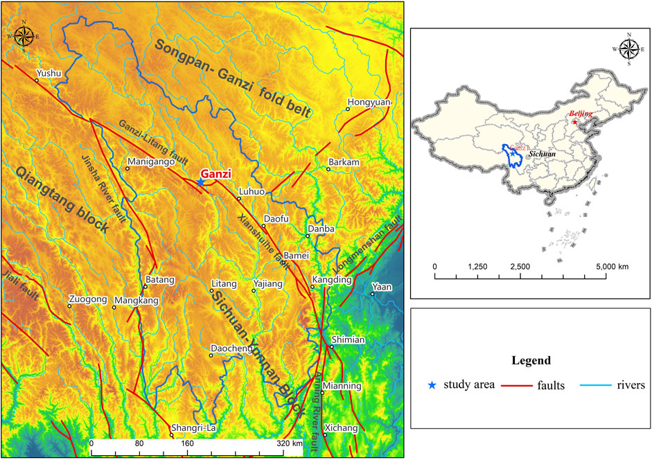
FIGURE 1. Geographical location of the study area.
Ganzi Tibetan Autonomous Prefecture is located in the extrusion and intersection zone of three tectonic units with different geotectonic characteristics, namely, the Eurasian plate, the Indian plate, and the Yangzi plate. The eastern Kangding–Luding area is located at the westernmost edge of the Yangtse plate and belongs to the northern section of the north–south tectonic zone of Kang-Dian. The western region is the easternmost edge of the Qinghai–Tibet plate that has the three major plates, especially the north and south of the two plates of multiple subductions—collision extrusion zone. Since the Paleozoic period, this region is still the most active area of neotectonic movements on the Qinghai–Tibet Plateau. There has been strong tectonic movement since the Paleozoic period, and because of the control of the boundary and subduction force of the three plates, the area is rapidly uplifted to become the highest terrain in the eastern part of the Tibetan Plateau; at the same time, because of the control of the direction of the plate suture zone and tectonic lines along the north–south direction, the mountains and water systems in the area are spread in a north–south direction, along the huge suture zone and tectonic lines which formed the famous Jinsha River, Yalong River, Xianshui River, Dadu River rift zone and its corresponding water system as well as the high mountain valley landscape. Influenced by the convergence–collision–mountain building of the Indian and Eurasian plates, many lithospheric scale strike-slip and retrograde fracture zones and volcanic island arcs have formed a plateau area with an average elevation of over 4000 m. Three deep and large fracture zones are developed in the region, namely, the Xianshui River Fracture Zone, the Ganzi–Litang Fracture Zone, and the Jinsha River Fracture Zone.
In different research fields, the Fourier transform has many different variant forms, such as the continuous Fourier transform and the discrete Fourier transform. It is based on the following principle: f(t) is a periodic function of t. If t satisfies the Dirichlet condition, in a period of 2T for f(x) continuous or only finite intermittent points of the first type, attached f(x) monotonic or divisible into finite monotonic intervals, then F(x) converges with a Fourier series of 2T for the period, and the function S(x) is also a periodic function of 2T for the period, and at these intermittent points, the function is finite-valued, has a finite number of extremal points in a period, and is absolutely productable, then Equation 1 holds (Liang et al., 2020). Eq. 1 is called the Fourier transform of the integral operation f(t), and the integral operation of Equation 2 is called the Fourier inverse transform of F(ω).
where F(ω) is called the image function of f(t) and f(t) is called the image original function of F(ω). f(ω) is the image of f (t). f(t) is the original image of F(ω).
The Fourier analysis used in this model is the fast Fourier transform (FFT), a method for quickly computing the discrete Fourier transform (DFT) or its inverse transform of a sequence. It is based on the principle of transforming a signal from the original domain (usually time or space) to a representation in the frequency domain or vice versa. The FFT will quickly compute such a transform by decomposing the DFT matrix into a product of sparse (mostly zero) factors. Thus, it is able to reduce the complexity of computing the DFT from O (N2), which is needed to compute it using only the DFT definition, to O
Soil temperature gradients are affected by seasonal and daily variations of solar illumination. Soil temperature gradients measured during fieldwork can only represent the temperature gradient at that time, but not the temperature gradient of the whole year, which is not important for the indication of annual heat dissipation, and a correction of the temperature gradient is needed to obtain an average surface temperature gradient on an interannual scale. In order to obtain stable values of the ground temperature gradient and conduct heat dissipation, the seasonal and diurnal effects of solar insolation on the ground temperature gradient can be corrected by our long-term temperature monitoring. We assume that the seasonal and daily variations of the atmospheric temperature can be synthesized in Fourier series form:
where T(0, t) is the temperature time series of the atmosphere, T0 is the average temperature of the atmosphere, Ai is the ith order amplitude, Pi is the ith order period, and φi is the ith order phase. We assume that the soil is homogeneous and that the heat transfer at depth is dominated by conduction. Through the one-dimensional heat conduction equation:
where κ is the soil thermal diffusion coefficient in m2/s and z is the depth in m. The time series of soil temperature affected by temperature change at any depth can be deduced as:
The above equation shows that soil temperature fluctuations decrease exponentially with increasing depth and show a phase lag, while they are both a function of period. The amplitude appears to decay with increasing depth, and the phase increases with depth. By comparing the equations, we can see that the temperature at any depth can be decomposed to represent the average temperature and the relative amplitude change at that depth, which is quite important for us to make temperature corrections later.
In contrast to direct measurements, indirect measurements of heat flow are usually used, and the two parameters mainly used for indirect measurements are the ground temperature gradient and the thermal conductivity of rocks. Based on the field monitoring results, this article uses the interannual average temperature gradient data to estimate the thermal conductivity by calculating the obtained soil thermal diffusivity. In the calculation of the measured heat flow, it is assumed that the heat transfer in the earth’s crust conforms to a bunch of Fourier’s laws of steady-state heat conduction, and the heat flow q is:
Soil thermal conductivity (K) indicates the characteristics of the soil when transferring heat, and the physical meaning is: the heat flux passed per unit time along the direction of heat transfer at a temperature difference of 1°C on both sides of a unit thickness of rock, numerically equal to the product of the thermal diffusion coefficient α, density ρ, and specific heat capacity c:
The data source of this experiment was selected from the measured temperature data collected in the field using self-developed probes from 1 November 2020 to 5 November 2021. Probe measurement is the measurement of temperature in the sediment using probes equipped with equally spaced temperature sensors to obtain temperature gradients. This equipment combined with the model proposed in this article can establish a geothermal flow measurement system based on low-temperature measurement and control in a borehole-free area to achieve convenient and efficient geothermal flow detection under low-temperature and low-power conditions. A total of four different depths of soil temperature data (20–50 cm) were collected and divided into four sets of temperature time series data for the purpose of experimental comparison and analysis. Details of the data are shown in Supplementary Table S1.
First, the temperature time series data need to be Fourier-transformed, the T-t data into complex (a+bi) form of spectral data, and then according to the Fourier transform requirements, combined with the linear interpolation approach to complete the data preprocessing. Since the prerequisite for the Fourier transform requires a sampled data size of 2n, we need to eliminate some of the sampled data, which may lead to temperature fluctuations with periods, amplitudes, and phases that may be more off the mark. However, due to the long monitoring time of this experiment and the fact that the actual number of deleted data represents less than 1% (1,082 samples were actually collected at each depth, with 1,024 remaining after deletion), this does not affect the results of this experiment too much. Using the Fourier-transformed data in complex form (a+bi), we calculate the period, amplitude, and phase of the temperature fluctuations that we really care about. The conversion relationship is as follows:
The imaginary part of the first complex point, b = 0, indicates a DC component (expanding the non-sinusoidal periodic signal by the Fourier series, the component with zero frequency), which in our case is actually the equilibrium temperature T0(z) at a depth unaffected by atmospheric temperature fluctuations, and the relationship between the remaining complexes is:
The relationship between the period Pi, amplitude Ai, and phase φi of the temperature fluctuation components and the complex number (a+bi) starting from the second complex point is as follows, where Ps is the actual sampling interval:
The temperature fluctuation period is the phase corresponding to the Pi component. ai>0,
The model built in this study has five panels (done using Python): data preprocessing, fast Fourier transform, solving the thermal diffusion coefficient, calculating the temperature time series, and plotting the temperature fluctuations (the detailed process of the whole model run is shown in the attached FFTcode.py). Regarding the solution of the soil thermal diffusion coefficient, after we get the period Pi, amplitude Ai, and phase φi of the desired temperature fluctuation components, in order to calculate the most suitable soil thermal diffusion coefficient, we use different values (here, we use 10−9–10−5 for a total of 12 values) to substitute into T(z, t), and then the solved time series T(z, t) of soil temperature affected by temperature change and the measured values were fitted with the variance(assume that 20 cm is the observed value and 30 cm is the measured value). We considered that the value of the thermal diffusion coefficient that obtained the minimum fitted variance was the most reasonable thermal diffusion coefficient for the soil between the two depths of 20 and 30 cm, and the variance fitting equation is as follows:
where yic and yim denote the calculated and measured temperatures at a depth of 30 cm, respectively. After obtaining what we consider to be the optimal thermal diffusion coefficient of the soil at 20 cm, the κ is substituted into T (z, t) to calculate the soil temperature time series T at a depth of 30 cm and then compared with the measured data temperature and analyzed the change of the two sets of data by comparing them by drawing a line graph to see whether the calculated soil temperature time series data eliminate the temperature fluctuations. Following the aforementioned method, we can calculate the soil temperature time series data at 30, 40, and 50 cm, so that we get three sets of theoretical optimal soil thermal diffusion coefficients at different depths and soil temperature data after correction for air temperature.
Through the variance fitting formula, we obtained the variance corresponding to different values of the three sets of data, and the details are shown in Table 1; then, the horizontal coordinate is κ, and the vertical coordinate is the variance plotted as a line graph, as in Figure 2. Through the graph of the thermal diffusion coefficient and fitted variance in Figure 2, we can choose the most suitable κ from the fitted κ graph for the next calculation, in which the two curves at the lowest point of the trend is the best value for the fit. We found that the two measured curves fluctuate in a similar trend, which also indicates that the results obtained from the two sides are correct and the optimal points of the values are similar, and the most suitable soil thermal diffusion coefficient (κ) is obtained to be approximately 6 × 10⁻⁷ m2/s.
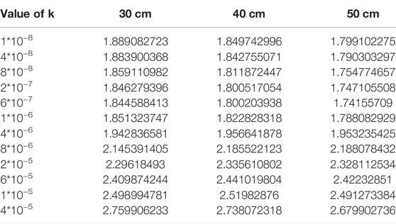
TABLE 1. Heat diffusion coefficient corresponding to the solution variance.
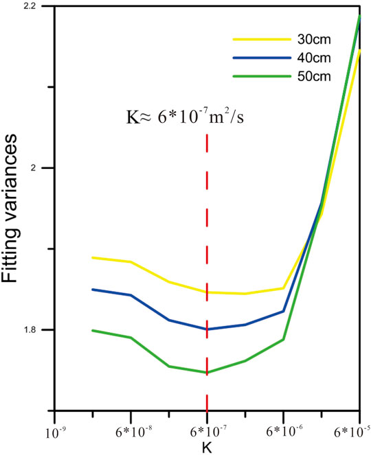
FIGURE 2. Fitted κ-value (for better visualization, only the first eight data are selected for the horizontal coordinates of the plot, which do not affect the results).
We made a temperature correction for the measured time temperature series of the original data, and the values of soil thermal diffusion coefficient (κ) were chosen to be 6 × 10⁻⁷ m2/s. Details of the time temperature series data before and after correction are shown in Supplementary Table S1, and then the line graphs were drawn as shown in Figure 3. Figure 3 shows the measured soil time temperature series data at different time periods and depths of 20–50 cm. It can be seen that the corrected temperature fluctuations are significantly reduced.
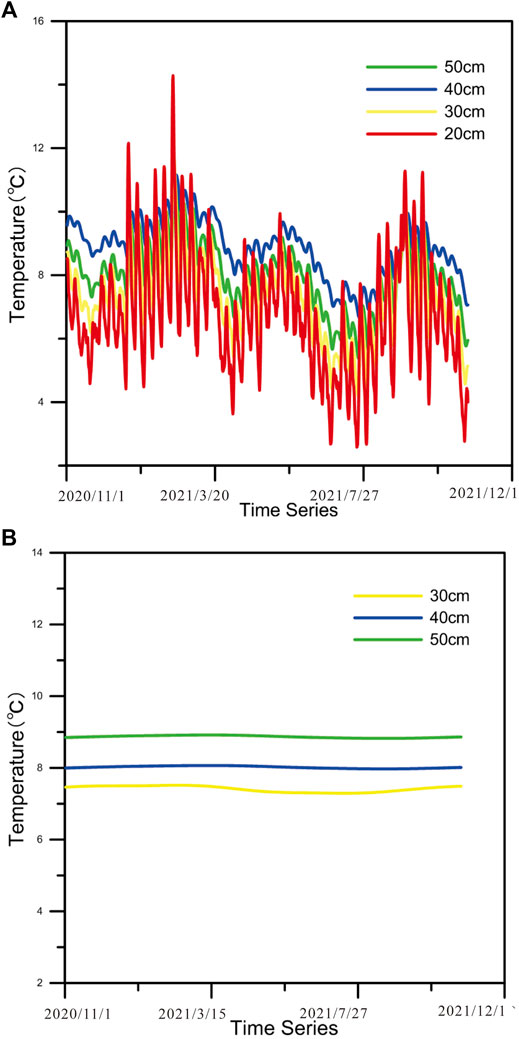
FIGURE 3. Measured temperature at different soil depths (A) and calculated results after temperature correction (B).
From the results in Figure 3, the fluctuation range of soil temperature at 20 cm before the correction was large, and the fluctuation range was 2.58°C–14.284°C, which was because the soil here was closer to the land surface and was affected too much by the temperature fluctuation, and as the soil depth deepened, the temperature fluctuation slowly became smaller, and the fluctuation range was 6.67°C–11.15°C at 50 cm, but the effect of temperature fluctuation was still obvious. Also, the fluctuation range was basically reduced to within 0.3°C after temperature correction.
From the analysis of the aforementioned experimental results, it can be seen that after correction for atmospheric temperature, the effect of temperature fluctuations is basically eliminated, so that the thermal diffusion coefficient of the soil at different depths can be obtained, and also the calculated temperatures at the corresponding depths can be obtained, as a way to presume the approximate geothermal gradient of the measured area. However, it needs to be recognized that this treatment of ours considers that the measured temperature is only influenced by diffusion and ignores the effect of convection. From the final results of the treatment, the deviation of the calculated results ignoring the effect of convection is not significant, and therefore, we believe that the effect of convection can be ignored in this experiment.
Geothermal heat flow is the basic physical parameter that characterizes the heat dissipation in the Earth by conduction. It is an indispensable parameter for studying the thermal state of the Earth’s interior, obtaining the temperature of the deep crust, and analyzing the thermal structure of the lithosphere, and it is a key parameter for assessing regional geothermal resources, and it can also provide basic parameters for the optimal selection of other new energy sources. It is also a direct display of the Earth’s internal thermal processes at the surface (or seafloor), which is not only a key data for understanding the rate of heat dissipation in the Earth but also a basic data for conducting kinetic studies and reconstructing the evolution of sedimentary basins and evaluating the potential of oil and gas and hydrate resources. Geothermal heat flow is important for the study of crustal activity, the thermal structure of the crust and upper mantle, and the evaluation of regional thermal state and geothermal resource potential (Qiu, 1998).
Usually, geothermal heat flow parameters depend on drilling conditions and can be obtained indirectly through geothermal temperature measurements and rock thermal conductivity tests, but in areas where drilling is lacking, geothermal heat flow is extremely difficult to obtain. The drilling temperature continuous acquisition system manufactured by R.G, United Kingdom, and the thermal conductivity scanner (TCS) made in Germany are the more commonly used temperature measurement and rock thermal conductivity testing equipment in China at present. Compared with rock thermal conductivity testing, temperature measurement requires more demanding conditions and requires the use of existing drilled wells, so it is limited in terms of quantity, spatial coverage, and depth. Influenced by the distribution of drilling wells, geothermal heat flow measurement points in China’s mainland are currently mainly distributed in the Sichuan Basin, Ordos Basin, Tarim Basin, and other hydrocarbon-bearing basins.
According to previous studies, the density of soils in the middle of the Ganzi County area is in the range of 0.94–1.56 g/cm3, and the specific heat capacity of soils is greatly influenced by the dryness and humidity of soils, and the geotechnical soils in the study area are mainly seasonal permafrost soils with local area soil representatives, and the specific heat capacity is taken as the average value of 1,741 kJ/m3∙K (Guo et al., 2014; Wang et al., 2014; Zhu et al., 2019; Yi et al., 2020). For the seasonal average temperature gradient data obtained in the field, it is necessary to take the temperature correction to eliminate the effect on soil temperature and then use it. The average of the corrected temperature data can better represent the temperature at that depth. After obtaining the corrected temperature at each depth, the variance of the temperature at the corresponding depth can be obtained at the same time. By doing the fitting curve of temperature versus depth, a better linear relationship was obtained for the temperature–depth profile. Therefore, the annual average ground temperature gradient can be obtained from the temperature–depth profile, and the seasonal average gradient in the study area obtained by removing the temperature influenced by temperature fluctuations is 7.3°C/m. According to Equations 7, 8, we can calculate the range of soil thermal conductivity as 0.986–1.585, and the preliminary heat flux Q is 9.3845 ± 2 W/m2.
The geothermal flux calculated in this way has a large error. We used the random sampling method to take 500 samples as experimental parameters in the derived soil thermal conductivity range to calculate the geothermal flux of the area, and then the results were randomly divided into five groups to calculate the standard error separately, and the group with the smaller error was taken as the final geothermal flux calculation result, and then its mean value was sought as the geothermal flux valuation of the study area. After the calculation, the sample group with the SE of 0.951 was selected as the experimental object, and the geothermal flux of the area was found to be 7.863 W/m2, and the details of the calculation are shown in Supplementary Table S2. Due to the limited number of field monitoring instruments, the experiment could not be conducted in more areas, and the lack of experimental data made it impossible to fit the total geothermal flux of the area. However, the method and the new model used in this study achieved good results in the experiments, which can also provide technical support for subsequent scholars to study the geothermal resources in the plateau region or to evaluate the geothermal potential of the region.
In this study, a new model is established based on Fourier analysis and heat conduction principle, and the long-term monitoring data of soil temperature in the field are processed, and two sets of temperature time series data measured at different soil depths are selected for experimental analysis, as a way to improve the calculation accuracy of soil conduction heat dissipation by eliminating the influence of temperature changes on soil temperature. The following preliminary conclusions were obtained:
1) From the results of tests on four groups of soils at different depths, the fluctuation range of soil temperature at 20 cm before the correction was large, and the fluctuation range was 2.58°C–14.284°C, and as the soil depth deepened, the temperature fluctuation slowly became smaller, and the fluctuation range was 6.67°C–11.15°C at 50 cm. Also, the fluctuation range was basically reduced to within 0.3°C after temperature correction. The results show that the influence of temperature variation on soil temperature has been eliminated as much as possible, which can provide help to improve the calculation accuracy of heat dissipation in the following calculations.
2) Through the seasonal average temperature data obtained in the field and previous research results, and then after eliminating the influence of temperature changes on soil temperature, the geothermal temperature gradient in the region can be calculated as 7.3°C/m and the geothermal flux valued as 7.863 W/m2. Although the number of monitoring points is not enough to fit the geothermal flux situation in the whole study area, the soil temperature time series processing method proposed in this study is feasible and can provide technical support for subsequent researchers to evaluate the geothermal situation in the region or to develop geothermal resources.
3) A model combining Fourier series analysis and heat conduction principle is established, which can realize the rapid processing of soil temperature time series, so as to obtain the soil thermal diffusion coefficient with high accuracy to correct the effect of temperature change on soil temperature, and the experimental results show that the accuracy of the correction is high, and the model is widely applicable, and the parameters can be adjusted according to the needs of researchers to improve the accuracy of the model in different areas of testing.
The original contributions presented in the study are included in the article/Supplementary Material; further inquiries can be directed to the corresponding author.
LYa: algorithm analysis, methodology, and writing—original draft. RS: writing—review and editing and methodology. BD: mapping and analysis of results. LYi: algorithm analysis and mapping. YF: writing—original draft and analysis of results. BZ: writing—review and editing and methodology. ZW: methodology and modeling. YW: writing—review and modeling. SD:review and editing.
This study was supported by the Joint Scientific Research Project of the Corporation (No. WWKY-2020-0103).
Authors LMY, LKY, YF, BZ, and ZW were employed by the company China Three Gorges Corporation.
The remaining authors declare that the research was conducted in the absence of any commercial or financial relationships that could be construed as a potential conflict of interest.
All claims expressed in this article are solely those of the authors and do not necessarily represent those of their affiliated organizations, or those of the publisher, the editors, and the reviewers. Any product that may be evaluated in this article, or claim that may be made by its manufacturer, is not guaranteed or endorsed by the publisher.
The Supplementary Material for this article can be found online at: https://www.frontiersin.org/articles/10.3389/feart.2022.910328/full#supplementary-material
Benseman, R. F. (1959). The Calorimetry of Steaming Ground in Thermal Areas. J. Geophys. Res. 64 (1), 123–126. doi:10.1029/jz064i001p00123
Coolbaugh, M., Sladek, C., Zehner, R., and Kratt, C. (2014). Shallow Temperature Surveys for Geothermal Exploration in the Great Basin, USA and Estimation of Shallow Convective Heat Loss. Geotherm. Resour. Counc. Trans. 38, 115–122. doi:10.1016/j.rse.2006.09.001
Dawson, G. B., and Author, A., (1970). Heat Flow Studies in Thermal Areas of the North Island of New Zealand. Geothermics, 2: 466–473. doi:10.1016/j.coldregions.2011
Domenico, P. A., and Schwartz, F. W. (1998). Physical and Chemical Hydrogeology. New York, NY: Wiley. doi:10.27671/d.cnki.gcjtc.2019.000407
Fridriksson, T., Kristjánsson, B. R., and Ármannsson, H. (2006). CO2 Emissions and Heat Flow through Soil, Fumaroles, and Steam Heated Mud Pools at the Reykjanes Geothermal Area, SW Iceland. Appl. Geochem. 21 (9), 1551–1569. doi:10.1016/j.apgeochem.2006.04.006
Guo, Y. (2014). Research on Vegetation Protection of Slope of Shima Highway in High Altitude and Cold Area. Chengdu, China: Chengdu University of Technology.
Holmes, T. R. H., Owe, M., De Jeu, R. A. M., and Kooi, H. (2008). Estimating the Soil Temperature Profile from a Single Depth Observation: a Simple Empirical Heatflow Solution. Water Resour. Res. 44 (2), 2412. doi:10.1029/2007wr005994
Horton, R., Wierenga, P. J., and Nielsen, D. R. (1983). Evaluation of Methods for Determining the Apparent Thermal-Diffusivity of Soil Near the Surface. Soil Sci. 47 (1), 25–32. doi:10.2136/sssaj1983.03615995004700010005x
Hu, G. J., Zhao, L., Wu, X. D., Li, R., Wu, T. H., Xie, C. W., et al. (2016). New Fourier-Series-Based Analytical Solution to the Conduction Convection Equation to Calculate Soil Temperature, Determine Soil Thermal Properties, or Estimate Water Flux. Int. J. Heat Mass Transf. 95, 815–823. doi:10.1016/j.ijheatmasstransfer.2015.11.078
Hurwitz, S., Harris, R. N., Werner, C. A., and Murphy, F. (2012). Heat Flow in Vapor Dominated Areas of the Yellowstone Plateau Volcanic Field: Implications for the Thermal Budget of the Yellowstone Caldera. J. Geophys. Res. Solid Earth 117 (B10). doi:10.1029/2012jb009463
LeSchack, L. A., and Lewis, J. E. (1983). Geothermal Prospecting with Shallo-Temp Surveys. Geophysics 48 (7), 975–996. doi:10.1190/1.1441523
Liang, K. M., Liu, F., Miao, G. Q., and Shao, L. B. (2020). Methods in Mathematical Physics. Beijing, China: Higher Education Press, 62–74.
Liang, S. J., Feng, B., and Yan, T. Z. (2018). Geothermal Resources and Their Development and Utilization. Environ. Dev. 30 (08), 247–249. doi:10.16647/j.cnki.cn15-1369/X.2018.08.150
Liu, S. H., Cui, Y., and Liu, H. P. (1991). Determination of Soil Thermal Diffusion Coefficient and its Application. J. Appl. Meteorology 04 (2), 337–345.
Ma, B., Jia, L. X., Yu, Y., Wang, H., Chen, J., Zhong, Si., et al. (2021). Earth Science and Carbon Neutrality: Current Status and Development Direction. Geol. China 48 (02), 347–358.
Qiu, N. S. (1998). Thermal Condition Profiles of Sedimentary Basins in Continental China. Adv. Earth Sci. (05), 34–38.
Ramos, M., de Pablo, M. A., Sebastian, E., Armiens, C., and Gómez-Elvira, J. (2012). Temperature Gradient Distribution in Permafrost Active Layer, Using a Prototype of the Ground Temperature Sensor (REMS-MSL) on Deception Island (Antarctica). Cold Regions Sci. Technol. 72, 23–32. doi:10.1016/j.coldregions.2011.10.012
Rissmann, C., Christenson, B., and Werner, C. (2012). Surface Heat Flow and CO2emissions within the Ohaaki Hydrothermal Field, Taupo Volcanic Zone, New Zealand. Appl. Geochem. 27 (1), 223–239. doi:10.1016/j.apgeochem.2011.10.006
Sorey, M. L., and Colvard, E. M. (1994). Measurements of Heat and Mass Flow from Thermal Areas in Lassen Volcanic National Park, California. Menlo Park, California: US Geological Survey.
Wang, L., Gao, Z., and Horton, R. (2010). Comparison of Six Algorithms to Determine the Soil Apparent Thermal Diffusivity at a Site in the Loess Plateau of China. Soil Sci. 175 (2), 51–60. doi:10.1097/ss.0b013e3181cdda3f
Wang, X., Xiang, C. H., Li, X. W., and Wen, D. J. (2014). Effects of Winter Fire on the Physicochemical Properties of Subalpine Meadow Soils in Western Sichuan. Grassl. Sci. 31 (05), 811–817.
Wang, Y. C., Li, L., Wen, H. G., and Hao, Y. L. (2022). Geochemical Evidence for the Nonexistence of Supercritical Geothermal Fluids at the Yangbajing Geothermal Field, Southern Tibet. J. Hydrology 604, 127243. doi:10.1016/j.jhydrol.2021.127243
Wang, J. Y., Qie, Z. H., Wu, T. Q., Liu, J. S., Wang, C., Wang, X. L., et al. (2021). Research on LSTM Neural Network for Soil Temperature Time Series Prediction. J. Anhui Agric. Univ. (05), 119–125. doi:10.13320/j.cnki.jauh.2021.0093
Wang, Y. C., Pang, Z. H., Hao, Y. L., Fan, Y. F., Tian, J., and Li, J. (2019). A Revised Method for Heat Flux Measurement with Applications to the Fracture Controlled Kangding Geothermal System in the Eastern Himalayan Syntaxis. Geothermics 77, 188–203. doi:10.1016/j.geothermics.2018.09.005
Wang, Y. C., and Pang, Z. H. (2021). Heat Flux Measurements and Thermal Potential of the Garze Geothermal Area in the Eastern Himalayan Syntaxis. J. Volcanol. Geotherm. Res. 420, 107407. doi:10.1016/j.jvolgeores.2021.107407
Yi, P. F. (2020). Hydrodynamic Mechanism of Subalpine Meadow Soil Slip Erosion and its Spatial Prediction and Evaluation. Chengdu, China: Chengdu University of Technology.
Zhu, R. (2019). Research on the Application of Foam Concrete for Roads in Monsoon Freeze Zone. Chongqing, China: Chongqing Jiaotong University.
Keywords: Ganzi county, geothermal resources, Fourier analysis, temperature time series, soil thermal diffusion coefficient
Citation: Yang L, Song R, Dong B, Yin L, Fan Y, Zhang B, Wang Z, Wang Y and Dong S (2022) Processing Method of Soil Temperature Time Series and Its Application in Geothermal Heat Flow. Front. Earth Sci. 10:910328. doi: 10.3389/feart.2022.910328
Received: 11 April 2022; Accepted: 29 April 2022;
Published: 17 June 2022.
Edited by:
Lidong Dai, Institute of Geochemistry (CAS), ChinaReviewed by:
Chang Su, Institute of Disaster Prevention, ChinaCopyright © 2022 Yang, Song, Dong, Yin, Fan, Zhang, Wang, Wang and Dong. This is an open-access article distributed under the terms of the Creative Commons Attribution License (CC BY). The use, distribution or reproduction in other forums is permitted, provided the original author(s) and the copyright owner(s) are credited and that the original publication in this journal is cited, in accordance with accepted academic practice. No use, distribution or reproduction is permitted which does not comply with these terms.
*Correspondence: Rongcai Song, NDE3MTAyMTQ1QHFxLmNvbQ==
Disclaimer: All claims expressed in this article are solely those of the authors and do not necessarily represent those of their affiliated organizations, or those of the publisher, the editors and the reviewers. Any product that may be evaluated in this article or claim that may be made by its manufacturer is not guaranteed or endorsed by the publisher.
Research integrity at Frontiers
Learn more about the work of our research integrity team to safeguard the quality of each article we publish.