Active Layer and Permafrost Investigations Using Geophysical and Geocryological Methods—A Case Study of the Khanovey Area, Near Vorkuta, in the NE European Russian Arctic

Permafrost in the NE European Russian Arctic is suffering from some of the highest degradation rates in the world. The rising mean annual air temperature causes warming permafrost, the increase in the active layer thickness (ALT), and the reduction of the permafrost extent. These phenomena represent a serious risk for infrastructures and human activities. ALT characterization is important to estimate the degree of permafrost degradation. We used a multidisciplinary approach to investigate the ALT distribution in the Khanovey railway station area (close to Vorkuta, Arctic Russia), where thaw subsidence leads to railroad vertical deformations up to 2.5 cm/year. Geocryological surveys, including vegetation analysis and underground temperature measurements, together with the faster and less invasive electrical resistivity tomography (ERT) geophysical method, were used to investigate the frozen/unfrozen ground settings between the railroad and the Vorkuta River. Borehole stratigraphy and landscape microzonation indicated a massive prevalence of clay and silty clay sediments at shallow depths in this area. The complex refractive index method (CRIM) was used to integrate and quantitatively validate the results. The data analysis showed landscape heterogeneity and maximum ALT and permafrost thickness values of about 7 and 50 m, respectively. The active layer was characterized by resistivity values ranging from about 30 to 100 Ωm, whereas the underlying permafrost resistivity exceeded 200 Ωm, up to a maximum of about 10 kΩm. In the active layer, there was a coexistence of frozen and unfrozen unconsolidated sediments, where the ice content estimated using the CRIM ranged from about 0.3 – 0.4 to 0.9. Moreover, the transition zone between the active layer base and the permafrost table, whose resistivity values ranged from 100 to 200 Ωm for this kind of sediments, showed ice contents ranging from 0.9 to 1.0. Taliks were present in some depressions of the study area, characterized by minimum resistivity values lower than 10 Ωm. This thermokarst activity was more active close to the railroad because of the absence of insulating vegetation. This study contributes to better understanding of the spatial variability of cryological conditions, and the result is helpful in addressing engineering solutions for the stability of the railway.

1 Introduction

Permafrost is defined as ground with a temperature remaining below 0°C for at least two consecutive years (ACGR—Associate Committee on Geotechnical Research, 1988; Isaev et al., 2020). Perennial frozen ground occupies around a quarter of the terrestrial surface in the Northern Hemisphere (Zhang et al., 1999; Gruber, 2012; Wang et al., 2019; Vasiliev et al., 2020) and more than 60% of the Russian territory (Anisimov and Reneva, 2006). The percentage of lateral continuity of permafrost can be classified into continuous (90–100%), discontinuous (50–90%), sporadic (10–50%), and isolated (<10%) (Brown et al., 1997; Brown et al., 2002). This distribution is represented in Figure 1 for the European Russian Arctic and Northwestern Siberia, a region experiencing some of the highest rates of permafrost degradation (Romanovsky et al., 2010; Streletskiy et al., 2015; Romanovsky et al., 2018; Biskaborn et al., 2019).

FIGURE 1

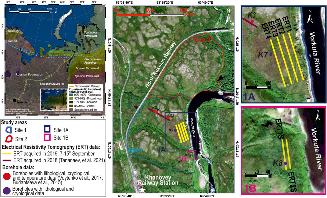
FIGURE 1. The top left map shows the location of the study area (Khanovey railway station, close to Vorkuta city) in the NE European Russian Arctic, along with the percentage of permafrost lateral continuity in the region (according to the classification of Brown et al., 1997; Brown et al., 2002). The map at the center of the figure shows the survey location area, with the position of boreholes and geophysical data used in this study. The profile positions of the geoelectric surveys performed in 2019 in Site 1A and Site 1B are highlighted in blow-ups on the right. Maps compiled using ArcGis^® (Esri) software. Datum: WGS84; projection: UTM 41N. Satellite base image (Gis layer “World Imagery”) and permafrost extent (Gis layer “North Hemisphere Permafrost_WFL1”) were retrieved in 2019 from the ArcGis online database resources.

The permafrost thermal state is highly sensitive to the changing climatic conditions (ACGR—Associate Committee on Geotechnical Research, 1988; Yershov, 1998; Harris et al., 2017; IPCC et al., 2017). The Arctic amplification, a proven phenomenon for which the Arctic is warming about twice as fast as the rest of the world, is altering the permafrost distribution and leading to its degradation (IPCC et al., 2017; Biskaborn et al., 2019; NOAA/NASA, 2020; NSIDC—National Snow and Ice Data Center, 2020). Several studies in the Eurasian Arctic (e.g., Streletskiy et al., 2015; Buldovicz et al., 2018; Romanovsky et al., 2018; Abramov et al., 2019; Maslakov et al., 2019) have already documented permafrost degradation induced by warming mean annual air temperatures (from 0.05 to 0.07°C yr⁻¹ since 1970; Vasiliev et al., 2020). In the Arctic Russia, permafrost is warming relatively slower than the Arctic air and it became about ∼1.5°C–2.5°C warmer during the last half-century (Biskaborn et al., 2019; Melnikov et al., 2022). As a consequence, the top layer of permafrost, subject to seasonal thawing and freezing (i.e., the active layer), increases its thickness (i.e., the active layer thickness—ALT), causing a northward retreat of permafrost extent and a widespread reduction in the capacity of soil to carry loads (Yershov, 1998; Osterkamp and Burn, 2003). Over the past 2 decades, ALT has increased at all Russian European Circumpolar-Active Layer-Monitoring (CALM) sites, showing strong positive trends varying from 0.3 to 3.0 cm per year (Kaverin et al., 2021). As the ground thaws and freezes, it contracts and expands, inducing subsidence (thaw settlement), stress on foundations, and surface deformation of infrastructures (Chen et al., 2014). This is due to the modification of the soil mechanical properties by thermokarst processes, leading to decreasing ground bearing effectiveness, which, in turn, produces deformation and collapse of buildings, bridges, roads, etc. (e.g., Hong et al., 2014; You et al., 2017).

These phenomena profoundly affect the natural Arctic environment, as well as most of the socio-economic sectors of northern communities (IPCC et al., 2017; Marohasy, 2017). More than half of the Arctic inhabitants live in Russian territories underlain by permafrost. Population density and socio-economic development levels are highly variable across the Russian Arctic (EEA—European Environment Agency, 2017; Hjort et al., 2022). Ranging from the largest cities (e.g., Vorkuta, Yakutsk, and Norilsk) to sparse and isolated villages, urbanized settlements are of various sizes, which are often related to the availability of basic resources for living and livelihood (Streletskiy and Shiklomanov, 2016; Streletskiy et al., 2019). However, the accessibility of these resources is becoming increasingly problematic. The systematic loss in the continuity of permafrost due to global warming presents serious problems because of the high costs of construction and infrastructure maintenance, limiting access to people and goods supply from and to the Arctic regions (Marohasy, 2017; Allen et al., 2018).

Permafrost degradation leads to serious consequences for ecosystems, hydrological systems, and infrastructure integrity. The most important are the following: greenhouse gases release (Yang et al., 2010; Streletskiy et al., 2015); slowly moving landslides (frozen debris lobes); coastal erosion (Kasprzak et al., 2017; Maslakov et al., 2019; Isaev et al., 2020; Sinitsyn et al., 2020); ground subsidence; and the decrease in bearing capacity (Streletskiy et al., 2015; Voytenko and Sergeev, 2016; Isaev et al., 2020). In particular, it causes damages to infrastructure networks (e.g., Chen et al., 2014), resulting in deformation and subsidence of railway line tracks (e.g., Figure 2). The presence of anomalous unfrozen ground zones close to the railroads, related to groundwater circulation and thermokarst processes, changes the thermal state of the ground and plays a huge role to infrastructure damage (e.g., Drozdov et al., 2015; Isaev et al., 2020; Hjort et al., 2022). This phenomenon produces a strong impact on economic costs for infrastructure maintenance (Voytenko et al., 2017; Streletskiy et al., 2019; Melnikov et al., 2022), rising the vulnerability of people and human activity.

FIGURE 2

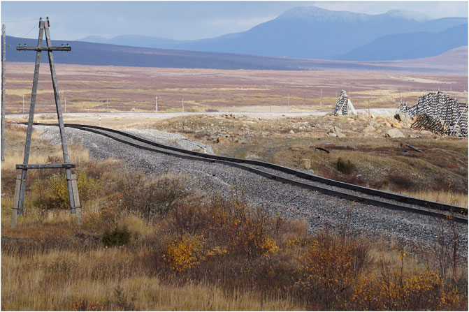
FIGURE 2. Railroad deformation associated with permafrost degradation along the North Russian Railway close to the Khanovey field site at the western foothills of the Ural Mountains.

Although climatic factors play major roles in explaining permafrost thickness and active layer trends across large regions, vegetation, soil properties (e.g., thermal capacity), and land-use are also influencing factors (Wagner et al., 2018; Vasiliev et al., 2020; Schneider von Deimling et al., 2021). Permafrost warming can be locally amplified as a consequence of construction operations, embankment geometry, snow accumulation on side slopes, or changes in material properties (Zhang et al., 2004; Vasiliev et al., 2020). The warming effects can worsen if inadequate construction methods and procedures are adopted, such as soil compaction, removal of peat, and destruction of the vegetation cover (Drozdov et al., 2015). Monitoring of the extension and thickness of permafrost and active layer by employing different investigation methodologies is fundamental for designing effective infrastructure consolidation plans and targeted solutions (e.g., Schwamborn et al., 2008; Voytenko and Sergeev, 2016; Gilbert et al., 2019; Tyurin et al., 2019).

A variety of methods commonly used for ALT and permafrost investigations can be found in the literature. Direct methods include mechanical probing, soil temperature monitoring, and visual observations (Hinkel and Nicholas, 1995; Brown et al., 2000). These methods form the basis of the CALM program (https://www2.gwu.edu/∼calm/), started in 1991 to study the impacts of climate change on permafrost environments (Brown et al., 2000; Hinkel and Nelson, 2003; Kaverin et al., 2021). Another direct method is the use of the annual thawing index based on surface air temperature data (e.g., Peng et al., 2016). In turn, modeling approaches have been applied to describe ALT variations at different spatial scales (Nelson et al., 1997; Nelson et al., 1999; Hinzman et al., 1998; Oelke et al., 2003; Sazonova and Romanovsky, 2003).

Regional active layer conditions are difficult to be determined from direct ground surveys of permafrost features (e.g., digging, core drilling, and temperature measurements in boreholes) because of the large permafrost extent, high costs, and inconsistent sampling (Duguay et al., 2005). As a consequence, indirect methods for regional ALT estimation are often employed, which provide near-surface indicators of underlying ground conditions. These methods consist in remote sensing observations (e.g., Yi and Kimball, 2020) incorporating different global satellite data (radar, microwave, and infrared) of vegetation cover, ground thermal (air and surface temperatures), and hydrological (snow depth and soil moisture) parameters in order to capture abrupt shifts in landscape properties between predominantly frozen and unfrozen conditions (Kimball et al., 2004; Kim et al., 2011; Park et al., 2016). Repeated observation at representative sites over long periods is essential to evaluate regional patterns and trends related to permafrost degradation.

Geophysical surveys, as ground-penetrating radar (GPR) and electrical resistivity tomography (ERT), have been extensively used to study active layer and permafrost features. However, although the GPR technique performs well only for low clay contents in the subsoil (e.g., Arcone and Delaney, 1982; Palacky, 1988; Delaney et al., 1990; Doolittle et al., 1990; Arcone et al., 1998; Hinkel et al., 2001), the ERT method enables the characterization of both the active layer and the underlying permafrost for almost all soil textures (e.g., Kasprzak, 2015; Seppi et al., 2015; Kasprzak et al., 2017; Léger et al., 2017; Picotti et al., 2017; Francese et al., 2019; Farzamian et al., 2020; Isaev et al., 2020). In addition, electromagnetic induction methods have been successfully used to estimate the thickness of permafrost (e.g., Isaev et al., 2020).

The purpose of this research is to integrate geophysical and geocryological methods for permafrost and ALT investigations in the northwestern European Arctic (Komi Republic). The target zone is the Khanovey railway station area, close to Vorkuta city, located on the west of the Ural Mountains (Figure 1). The study area, characterized by Quaternary sediments lying on Permian coal shale bedrock, exhibits a continuous permafrost layer (Tananaev et al., 2021). This region is crossed by the North Russian Railway, which represents the only land connection between Moscow city and the northern Arctic territories. Several studies report that this important railroad infrastructure is suffering from deformation reaching 2.5 cm yr⁻¹ due to the thawing of permafrost (e.g., Voytenko and Sergeev, 2016; Vasiliev et al., 2020). At the nearby Talnik CALM site, the average ALT increased steadily in the 1998–2019 period from 76 to 152 cm, showing a site-averaged trend of 4 cm yr⁻¹ (Kaverin et al., 2021).

This research encompasses engineering/geocryological surveys (borehole drilling and thermometry), geophysical surveys (geoelectric), landscape microzonation, and digital mapping. These investigation methods provided data with different resolutions, which were combined together to characterize the unfrozen and frozen ground thickness distribution in the Khanovey field site. The complex refractive index method (CRIM) rock-physics theory has also been applied to enhance data integration and to quantitatively validate the geophysical results. This research is useful to address engineering solutions that ensure stability and operational performance to the railway, e.g., railway line diversion or employment of the thermosyphon and insulation cover technologies (e.g., Wagner, 2014; Isaev et al., 2016; Ulyanov, 2021).

2 Area Description

The investigated area is located in the Bolshezemelskaya tundra, about 60 km west of the foothills of the Ural Mountains. It has an extension of approximately 1 km², and it is delimited by the Vorkuta riverbank on the eastern side and by the North Russian Railway on the western side. It was subdivided into two parts: the southern area (Site 1, delimited by the light blue line in the map of Figure 1), the main target of this study, and the northern area (Site 2, delimited by the red line in the map of Figure 1), where geocryological data were collected in 2019 for future geophysical investigations. In Site 1, the geological, cryological, and geophysical data were collected in 2019 and previous years.

With respect to orography, the territory is an accumulative plain, with an absolute surface at 70–200 m above sea level (a.s.l.) and erosions within the plains, with depths of 20–40 m (Isaev V. S. et al., 2022). In landscape terms, the site is characterized by a peaty-bumpy tundra, which is a system of microdepressions and hollows interspersed by hillocks.

The Khanovey study area is part of the Timan–Pechora sedimentary basin, which belongs to the submerged north-eastern part of the European Platform. More into detail, the site is settled over the tectonic unit of the Pre-Urals Foredeep (Klimenko et al., 2011). The sedimentary sequence of the area consists of Silurian siliceous shale deposits that originate at the initial stage of formation of the young Timan–Pechora platform, lying at a depth of approximately 250 m. These sediments are covered by lower Carboniferous coal, dolomite, and limestone (Vorgashorskaya Formation) emerging at a depth of about 50 m. Lower Permian sediments are constituted by about 15 m thick alternation of sandstone, siltstone, and mudstone (Artinskian Stage) and by about 4–20 m coal layers (Kungurian Stage). Quaternary sediments are represented by Middle Pleistocene marine and ice-marine deposits (loam and silt of yellow-brown color) and Upper Pleistocene and Holocene alluvial sediments. The total thickness of the Quaternary sediments is 15–30 m, with an average of 20 m (USSR Engineering Geology, 1991; Isaev V. S. et al., 2022). These alluvial and moraine deposits are the basement of the railway embankment throughout the surveyed area (Vasiliev et al., 2020). They lie on the lower frozen Carboniferous coal deposits of the Vorgashorskaya Formation that crop out on the riverbanks of the Vorkuta River (Isaev V. S. et al., 2022).

Regional climate has a Subarctic character: summer is short and cool, and winter is long and cold, lasting over 8 months from October to May. The total period without negative daily temperatures is only 70 days in average per year, and the mean annual daily temperature is −5.6°C (Tananaev et al., 2021). Total annual snow accumulation is increasing. Precipitation is about 430 mm, of which from 50% to 70% fall as snow (Tananaev et al., 2021). In tundra landscape, snow accumulation increased by 1.8 cm yr⁻¹ over the period 1998–2018 (Vasiliev et al., 2020).

The thickness of permafrost in this area was estimated to range between 40 and 95 m using the near-field transient electromagnetic sounding method (Isaev et al., 2020). Railway engineering service confirmed these values by means of seismic data analysis and core drilling operations.

The maximum annual ground temperature ranges between −0.5°C and −1.0°C at zero annual amplitude depth (around 12 m, Tananaev et al., 2021). A residual thaw layer is occurring annually between the base of the seasonally freezing layer at 2–3 m depth and the top of the permafrost layer at 4–5 m depth (Tananaev et al., 2021). Important cryogenic processes occur, including thermokarst and fluvial thermal erosion. Frost boils are also common cryogenic features, mostly occurring in a narrow belt surrounding the water track valleys (Tananaev et al., 2021).

Of particular interest is the diffuse presence of thermokarst phenomena. Thermokarst is a permafrost degradation process initially caused by a disruption of the ground thermal equilibrium that increases the ALT (Jorgenson, 2022). The land surface expression of this process is a thermokarst area generally characterized by marshy hollows. The progressive permafrost degradation can evolve in the development of a closed or an open talik, i.e., an anomalous unfrozen ground enclosed in permafrost or open to the surface, respectively. Further melting of ground ice leads to complete degradation, with all permafrost thawed. In this case, the thermokarst process degenerates to the development of a deep (or through) talik, without permafrost either at the top or the bottom (Jorgenson, 2022). The land surface expression of taliks generally consists in shallow thermokarst lakes and rivers, particularly in regions of continuous permafrost. In the case of deep taliks, the presence of thermokarst lakes depends on the type of soil. Often, both the surface water and the pore water in the underneath sediments do not freeze in winter.

The Khanovey site is an example of a permafrost degradation process at a metastable stage, referred to as “climate-driven, ecosystem-protected permafrost” (Vasiliev et al., 2020). Melting of ground ice near the permafrost table produces uneven thaw and thermokarst, affecting infrastructure and engineering constructions. Here, permafrost degradation and the gradual lowering of the permafrost table lead to vertical deformation (up to 2.5 cm yr⁻¹) of the North Russian Railway roadbed (Figure 2), a process accelerated by the removal of peat during the construction, with a consequent change of the local thermal regime (Voytenko and Sergeev, 2016; Vasiliev et al., 2020).

3 Methods and Datasets

Data were mostly acquired at the end of the warm season, between 1 and 23 September 2019, during the international educational course “Vorkuta Engineer-Geocryological Field Work” held by Lomonosov Moscow State University–MSU in collaboration with Norwegian University of Science and Technology–NTNU. The late summer period guarantees the collection of data on the maximum annual thickness of the active layer. Several direct and indirect surveys were carried out and integrated together for a detailed ALT mapping.

Geocryological and landscape surveys, in accordance with Russian standards of permafrost investigations, encompassed borehole coring, probing, and digital mapping. These measurements allowed the subdivision of the area into zones as a function of size relief, geomorphological characteristic, slope exposition, vegetation cover, drainage condition, ALT direct estimates, lithology, and cryogenic processes (e.g., thermokarst, frost heaving, frost boil, and solifluction).

Since 2012, several boreholes have been drilled within the study area, which provide useful lithological information. Furthermore, thermometric sensors were installed in 2015, and ground temperatures profiles were reconstructed using records from 2015 to 2018. Information from three boreholes was used in this study to calibrate the geophysical data.

Indirect geophysical investigations were carried out to integrate the geocryological and landscape data. The geoelectric method was used for frozen and unfrozen ground characterization, which included the ice content estimation in the active layer and the ALT mapping. Previous and new geoelectric profiles (Figure 1) were combined with ground thermometry and borehole data to get information about the frozen and unfrozen ground distribution between the railway and the Vorkuta River.

Thermometric measurements in boreholes, core lithologies, geophysical surveys, drilling, and probing have been carried out in Site 1. Geophysical surveys consist in geoelectric measurements, as an integration to the previous geoelectric survey (September 2018), to map the distribution of permafrost and of the active layer. New landscape zonation and geophysical investigations were conducted during the September 2019 field work to integrate the satellite images and data of previous surveys (e.g., ground temperature measurements, borehole information, and geoelectric data). Two areas were selected for the geoelectric acquisitions within Site 1, both near the western Vorkuta riverbank: Site 1A to the north and Site 1B to the south (Figure 1). Site 2 was an unexplored area until September 2019, when only a landscape survey was performed.

The combination of all methods employed in this study provided investigations at different resolutions, allowing the characterization of the unfrozen and frozen patterns and thickness distribution from the surface up to tens of meters depth. Furthermore, it is essential to distinguish between different types of taliks in thermokarst areas. Taliks are bodies of unfrozen ground occurring in a permafrost area due to a local anomaly in ground thermal conditions. They can be closed, open, or deep (through), depending on whether the talik is surrounded by permafrost, open at the top, or open both at the top and the bottom. Geophysical methodologies are fundamental for the detection and differentiation of these features and for defining the rock-physical properties of the frozen soil. In this perspective, the CRIM rock-physics theory can be very useful to link the underground resistivity values to the petrophysical properties (porosity, clay, and ice content) and to enhance integration among the results from geophysical and other surveys (core lithologies, thermometric data, and landscape zonation).

3.1 Geocryological Survey and Landscape Microzonation

Satellite images (of year 2019) were interpreted to preliminarily identify the main morphological elements such as the following: water streams, depressions, hilltops with different vegetation, river embankments, river terraces, anthropogenic structures (such as buildings, railroads, and pits), lakes, channels, and gully erosions. Correlations among landscape type, color and tone, texture, shape, and size of areas were applied to perform this analysis (according to Jensen, 2007).

Moreover, a geocryological field survey (Yershov, 1998) encompassed direct sampling and observation at 73 and 14 points within Site 1 and Site 2, respectively. The following types of information were identified and collected:

- relief surface characteristics. Mesorelief > 2 m height above mean topography (a.m.t.), which is about 85 m a.s.l.; microrelief < 2 m height a.m.t., defined as flat or moundy. When moundy, the height of the mounds is reported;

- surface drainage type (swamp, stream, wet, moist, dry, and very dry);

- vegetation type (lichen, moss, shrub, shrubbish, bush, and grass), according to Goryachkin et al. (1994);

- surface soil sediment classification on a texture basis (clay, silty clay, silty sand, sand, gravel, pebble, and cobble), according to the Folk diagram (Folk, 1954);

- cryogenic processes, such as thermokarst phenomena, frost heaving (i.e., upward or downward displacement of the ground surface caused by freezing and thawing of water in soil), and frost boil (i.e., nonsorted circles resulting from deformation and mixing soils caused by frost heave during freeze back of the active layer);

- morphological elements/processes: river terraces, gully erosion, and solifluction (i.e., slow downhill flow of saturated soil).

Direct estimations of ALT were also performed by digging and probing with a 2 m long metallic probe, in accordance with CALM methodology. Shovel excavations (until 1.50 m depth) allowed us to analyze the cryolithology of seasonally thawing/freezing sediments.

The collected morphological (both from preliminary analysis of satellite image and from direct field survey) and geocryological data (field survey), together with classified landscape microzones, were cataloged and digitalized as georeferenced layers using the ArcGIS^® (Esri) software to produce the geocryological and landscape microzonation map.

3.2 Boreholes and Temperature Measurements

Between 2012 and 2018, eight boreholes were drilled in the Khanovey area. Five of these boreholes are of particular interest for this study: K1, K2, K3, K7, and K8 (Figure 1). K1 and K2 were drilled in 2014 down to depths of 4.85 and 4.80 m, respectively. Borehole K3 was drilled in 2015 down to a depth of 5.80 m. Borehole K7 was executed in 2017 down to a depth of 2.90 m, and K8 was executed in 2018 down to a depth of 4 m. Rotational or rotational-pressure drilling methods were employed. Rotary core drilling was carried out with the help of a motorized drill for a maximum investigation depth of each borehole. Lithological and geocryological information are available for all five boreholes, from the top to the bottom of the holes (Voytenko et al., 2017).

To analyze the thermal conductivity of the shallower soil, ground temperatures were recorded from October 2015 to October 2018 using a thermistor set composed of GeoPrecision Logger Thermistor strings (https://www.thermistor-string.com/) and Hobo Thermistor strings (https://www.onsetcomp.com/products/sensors/s-tmb-m0xx/) installed in boreholes K1, K2, and K3.

3.3 Geophysical Surveys

Thawing permafrost is strongly linked to local scale changes in the rock-physical properties of frozen soil, which can be monitored using geophysical and geocryological methods. The degree of freezing of interstitial water has a negligible effect on density and magnetic permeability, precluding the use of gravimetric and magnetic techniques. It is fortunate that freezing has a marked effect on dielectric permittivity (Thomson et al., 2012), conductivity (Palacky, 1988; Seppi et al., 2015; Picotti et al., 2017; Francese et al., 2019), and seismic wave velocities (Carcione and Seriani, 1998). Hence, geoelectric, electromagnetic, and seismic methods constitute the best approaches to quantify the thawing degree of ice in sediments.

In this work, geophysical investigations were performed by acquiring both geoelectric and GPR profiles. Although the study area posed severe limits to the GPR technique due to the presence of massive clay contents in the subsoil, the geoelectric method enabled us to characterize both the shallow unfrozen and deep frozen ground, as well as the ALT. The geoelectric method can accurately distinguish between frozen and unfrozen soil based on the spatial variations of resistivity. ERT has been proven to be the most effective technique for monitoring ice content because upon freezing, electrolytic conduction is suppressed, reducing ion mobility and implying a marked increase in the resistivity of the ground (Palacky, 1988; Petrenko and Whitworth, 2002).

3.3.1 Geoelectric Data Acquisition

An IRIS Syscal Pro electrical resistivity meter, an all-in-one multinode resistivity system, was used for geoelectric field acquisition. The combination of both the dipole–dipole and pole–dipole configurations ensures high sensitivity to lateral and vertical resistivity variations, as well as a good signal-to-noise ratio and penetration. A total of six geoelectric profiles were acquired from 7 to 15 September 2019 in Site 1A and Site 1B (Figure 1). The interest in these two sites is due to the fact that a wildfire occurred a few decades ago in the former and a new borehole is planned in the latter. Four parallel 240 m long profiles (ERT1, ERT2, ERT3, and ERT4) were recorded in Site 1A using a 5 m electrode spacing. Two parallel 48 m long profiles (ERT1S and ERT2S) were acquired in Site 1B using a 1 m electrode spacing. The lines were oriented in the NW–SE direction in Site 1A and approximately in the N–S direction in Site 1B. In the latter, only the dipole–dipole configuration was used for both lines.

3.3.2 Geoelectric Data Processing and Electrical Resistivity Tomography

The geoelectric data were processed and inverted by adopting ERTLab™—ViewLab3D™ (http://www.geostudiastier.it/) package. Prior to the inversion procedure for the production of the resistivity model (imaging), the dataset was subjected to quality control. Overall, the dataset was of excellent quality, and for this reason, only 1% of the total quadrupoles were removed. Data processing was based on the following criteria (e.g., Seppi et al., 2015; Picotti et al., 2017): elimination of measurements with instrumental standard deviation (obtained through multiple measurement stacks) larger than 10%, removal of the receiver potentials lower (in absolute value) than 0.01 mV, and filtering of negative apparent resistivity values (that have physical meaning only in 3D surveys).

Figure 3 shows the histograms of the statistical distribution of the potentials, currents, and apparent resistivities after filtering. The currents injected at the transmission electrodes had an average value of about 72 mA, and the average apparent resistivity value was around 200 Ωm.

FIGURE 3

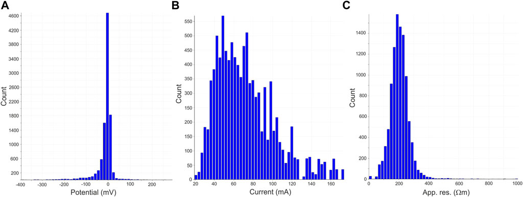
FIGURE 3. Histograms of (A) potentials, (B) injected currents, and (C) apparent resistivities.

The processed data were then inverted in order to perform imaging and obtain a realistic distribution of subsoil resistivity. The inversion parameters were the following:

- mesh size in the x and z directions equal to half of the electrode spacing: 2.5 m in Site 1A and 0.5 m in Site 1B;

- initial homogeneous resistivity model equal to the average of the apparent resistivity values;

- noise level of 3%, estimated via a statistical analysis of the reciprocal measurements.

Tomographic inversion converged after a maximum of four iterations for all considered datasets.

The ERT was carried out also using another software, the Geotomo Res2dInv (https://www.geotomosoft.com/) package, leading to very similar results. The resulting ERT sections were then interpreted using the Kingdom™ (IHS Markit) and ArcGIS^® (Esri) packages to produce the ALT map and integrate together the geocryological and geophysical results.

4 Results

4.1 Landscape Zonation

On the basis of the morphological and geocryological investigations, 12 different types of landscape microzones were classified in both Site 1 and Site 2 (Figure 4). The 12 classified microzones were the following: moundy hilltop, mixed hilltop, even hilltop, bushy depression, swamp depression (Figures 5A, B), even hillslope (Figure 5C), flat hilltop (Figure 5D), moundy hillslope (Figure 5E), riverbank (Figure 5F) and riverbank landslide, valley, and anthropogenic area (e.g., Figures 2, 5A).

FIGURE 4

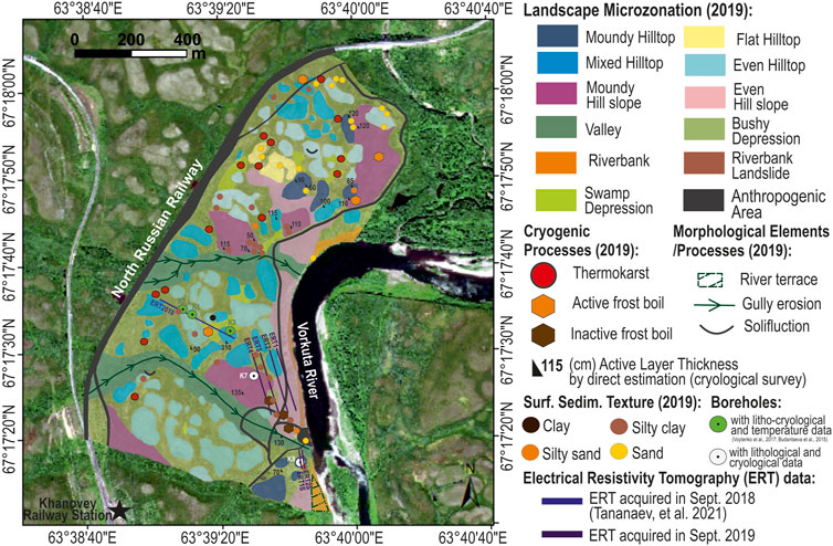
FIGURE 4. Landscape microzonation map resulting from the morphological analysis and geocryological survey in September 2019 in the Khanovey study area. The position of boreholes and geophysical profiles used in this study are also shown. Silty clay deposits (brown dots) represent the major soil sediment texture type, except for the riverbank and for the northern sector, where abundant sand deposits are present (yellow dots). The active layer thickness values (direct estimations) are indicated by black triangles. Thermokarst phenomena, mainly located close to the railway embankments, is indicated by red dots; solifluction, inactive and active frost boils, gully erosion, and river terrace are also displayed. The surveyed area can be subdivided into 12 different landscapes as indicated in the legend and in Table 1. Map compiled using ArcGis^® (Esri) software. Datum: WGS84; projection: UTM 41N. Satellite base image (Gis layer “World Imagery”) retrieved in 2019 from the ArcGis online database resources.

FIGURE 5

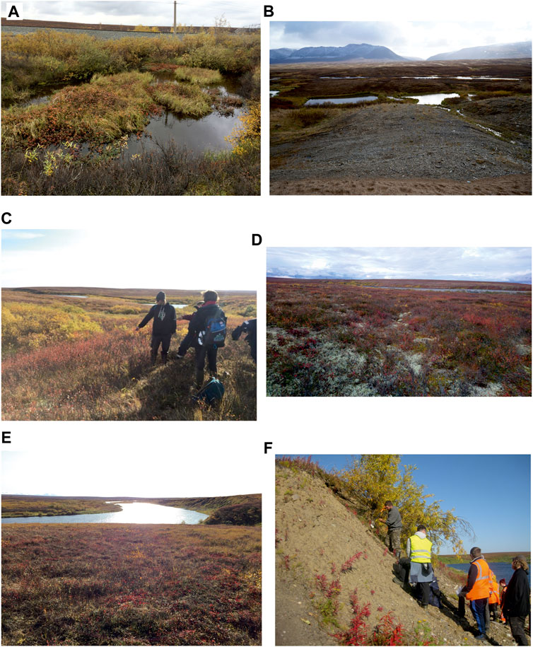
FIGURE 5. (A) thermokarst phenomena close to the railway. (B) thermokarst phenomena, within bushy and swamp depressions, that mark the Arctic landscape at the western foothills of the Ural Mountains. (C) even hillslope landscape characterized by small mounds (maximum 20 cm high) covered by lichen (e.g., reindeer lichens, in white) and small shrubs (e.g., Vaccinium myrtillus or blueberry) vegetation. (D) flat hilltop landscape example, close to the railway, mainly characterized by lichen (e.g., reindeer lichen, in white), small shrub (e.g., Rhododendron tomentosum or Labrador tea), and few amount of moss vegetation. (E) moundy hillslope landscape with massive mounds about 25–50 cm high covered by lichen, dwarf birch, moss, and grass. Wet intermound depressions are also abundant. (F) vorkuta riverbank covered by patches of grass and, in this case, an isolated tree.

The peculiar characteristics of each microzone are summarized in Table 1, and Figure 4 displays the geocryological features and the landscape microzonation map performed for the surveyed area (both Site 1 and Site 2).

TABLE 1

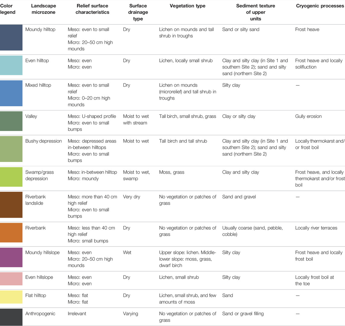
TABLE 1. Characteristics of the 12 different types of landscape microzones identified in the Khanovey area (Site 1 and Site 2) by the geocryological survey. The main types of surface relief, drainage, vegetation, surface sediment texture classification, and cryogenic processes are reported.

The land surface is characterized by large polygonal features, with a diameter between about 10 and 150 m. Mesorelief (>2 m height a.m.t.) and microrelief (<2 m height a.m.t.) are typical of the area. The hill landscapes (hilltop and hillslope) are classified on the basis of the shape and slope pattern as follows: flat, moundy, even (uniform hill), and mixed. The term “moundy” refers to a rugged and irregular hill with mounds up to about 20–50 cm a.m.t. high. The main difference between moundy and mixed hill is due to the vegetation pattern and smaller mound height (up to 20 cm a.m.t.) in mixed hill. Depressions are subdivided according to the vegetation type into the following: bushy (characterized by tall shrubs and birches) and swamp/grass depressions (characterized by moss and grass). Flat areas of flood plain and a river terrace are present in the southern eastern sector of Site 1, both covered by grass. The anthropogenic area, usually characterized by sand and gravel, includes railroad, pathways, the base camp set up during the field work, the coal pit, and the pump station.

The study area is covered by unconsolidated fine-grained sediments related to Quaternary glaciomarine deposits. Clay and silty clay sediments are dominant, except for the riverbank and the northern sector of Site 2, where sand and silty sand deposits dominate the moundy, even, and flat hilltops. At the toe of the even hillslope, occasional clasts of pebble to cobble size can be found. Two interpretations can explain this: uprising of the coarse grains due to the frost heave phenomena or fluvial deposit associated with the adjacent valley.

Within the valley landscape (covered by clay and silty clay), gullies erosion with U-shaped profiles are characterized by stream surface drainage and small waterfalls that evidence a recent development. The riverbank landslide consists of sand and gravel. Along the Vorkuta River, riverbanks form an about 45° slope (Figure 5F). In the riverbank area, a shallow study section, dug by shovel and less than 2 m deep, reveals that the uppermost sediments are dominated by sandy loam, mainly massive, with occasional clasts of pebble to cobble size and iron precipitations. Striated clasts indicate that the sediment is evidently of glacial origin. A deeper laminated coarse sand unit, with clasts of pebble to cobble size, is present. Grain size rapidly declines away from the riverbank, with sediments becoming finer.

Hilltops with <1° slope (e.g., even hilltop) are associated with phenomena related to seasonal freeze–thaw, which saturates the soil on the surface and induces solifluction movements along the slope. Thermokarst phenomena (Figures 5A, B) and frost boils are cryogenic processes associated with permafrost. Frost boils are subdivided into active and inactive (covered by vegetation). In the latter, the interrupted frost heaving due to the increase in the thaw layer allows plants to encroach the area. Thermokarst areas usually develop close to the eastern side of the railroad (Figure 4) because of the vegetation layer removal during the construction of embankments.

The tundra vegetation of the study area is mainly constituted by lichen, moss, grass, tall and small shrubs, and dwarf and tall birches. There are no forest trees, except a few trees grown in the valley. Moss (e.g., Myosotis asiatica and the Saxifraga and Sphagnum genera) grows in wet areas typically characterizing the swamp depression, moundy hillslope, but is lesser in flat hilltop. Grass (e.g., Equisetum arvense or Carex) grows in wet areas too, such as swamp depressions, valley, and moundy hillslopes, and locally in the riverbank. Moreover, grass outlines thermokarst areas, where the depressed land is soaked in water (Figures 5A, B). Lichen (e.g., Cladonia rangiferina, known also as reindeer lichen) dominates dry surfaces, such as hilltops and the upper part of the even and moundy hillslopes. Small shrubs (e.g., Rhododendron tomentosum or Labrador tea, Salix arctica or Arctic willow, Vaccinium myrtillus or blackberry, Vaccinium cyanococcus or blueberry, Vaccinium vitis-idaea or lingonberry, Arctostaphylos uva-ursi or bearberry, and Empetrum nigrum or crowberry) are adapted to live in both dry and wet surface areas, like flat and even hilltops, even hillslope and the valley, whereas tall shrubs are present only within wet environments as troughs of mixed hilltop and bushy depressions. Tall birches (Betula glandulosa) and dwarf birches (Betula nana) grow in moist to wet landscapes, with the former in valley and bushy depression and the latter in moundy middle-lower slope.

ALT direct estimations showed an average value of about 1 m, with values ranging from 0.5 to 3.1 m, but these measurements are not reliable because ALT could be larger than that directly estimated, due to the limits of the digging and/or probing methods and/or the possible presence of taliks. The geocryological features and the landscape microzonation map performed for the surveyed area (both Site 1 and Site 2) are displayed in Figure 4.

4.2 Ground Thermometry and Coring

Temperature data for at least two consecutive years (2016–2018) are available only for boreholes K1, K2, and K3. The lithological and vertical ground temperature profiles corresponding to these boreholes are shown in Figures 6A, B, respectively. Figure 6B shows the annual maximum, minimum, and mean temperature curves together with the permafrost table depth (where detectable), which corresponds to the surface where the temperature is always under 0°C. In general, the measurements show that in the active layer, the temperature reaches a maximum value of about 18°C during summer and a minimum value down to less than −5°C during winter. K1 and K3 boreholes show larger temperature fluctuations near the surface, where the thermal heat transfer is more intense. The permafrost table is clearly identified only at the bottom of borehole K1, at about 4.8 m depth (Figure 6B), where the temperature is always below 0°C and massive cryogenic structures are present in the lithological profiles. The active layer and unfrozen ground bottom are identified in boreholes K1 and K3, at depths of about 3.7 and 4.7 m, respectively, and coincide with the presence of frozen sediments in the lithological profiles and temperatures around 0°C. The bottom of the K3 borehole shows temperatures very close to 0°C, and the permafrost table cannot be clearly identified. On the other hand, borehole K2 exhibits only positive temperatures. Here, the total absence of cryogenic structures (Figure 6A) confirms that a deep unfrozen ground (a talik) dominates the area.

FIGURE 6

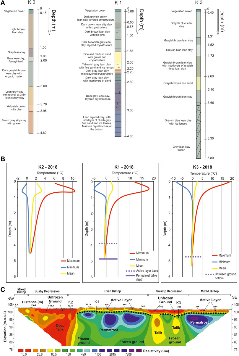
FIGURE 6. (A) lithological and geocryological core analysis of boreholes K1, K2, and K3 (data from Budantseva et al., 2015; Voytenko et al., 2017). (B) maximum, minimum, and mean temperature curves of the year 2018, where the unfrozen ground bottom, the active layer bottom, and the permafrost table depth are indicated. (C) interpretation of the ERT2018 resistivity section (modified from Tananaev et al., 2021), crossing boreholes K1, K2, and K3. The interpretation of the active layer and unfrozen ground bottom (black dashed line), marked by the resistivity value of 100 Ωm, is in agreement with the core analysis and with the temperature profiles at K1 and K3. Wide temperature fluctuations occur in the active layer, characterized by low resistivity values (ρ < 100 Ωm). A deep talik is present in the NW sector, explaining the unusual trend in the temperature profile of the K2 borehole. Two taliks enclosed in the frozen ground are present beneath the swamp depression zone, between K1 and K3 (ρ < 80 Ωm), covered by a 3 m thick unfrozen ground layer. One of the two taliks is open to the surface.

Borehole stratigraphy shows that clay and silty clay sediments are dominant, confirming the results of landscape zonation. Core samples often exhibit a layered cryostructure along boreholes K1 and K3.

4.3 Electrical Resistivity Tomography Sections

The ERT profiles in the study sites are interpreted and integrated with the geocryological data, landscape zonation (Figure 4), and borehole data. Lithological data are available for boreholes K1, K2, and K3 (Figure 6A), located along a previous geoelectric survey (profile ERT2018, Figure 6C) acquired in September 2018 (Isaev et al., 2020), and for boreholes K7 and K8 (Figure 7C), located on profiles ERT4 (Figure 7A) and ERT1S (Figure 7B), respectively. The ERT2018 section was obtained using the Geotomo Res2dInv package. The acquisition and processing of the ERT2018 profile are described by Isaev et al. (2020) and Tananaev et al. (2021).

FIGURE 7

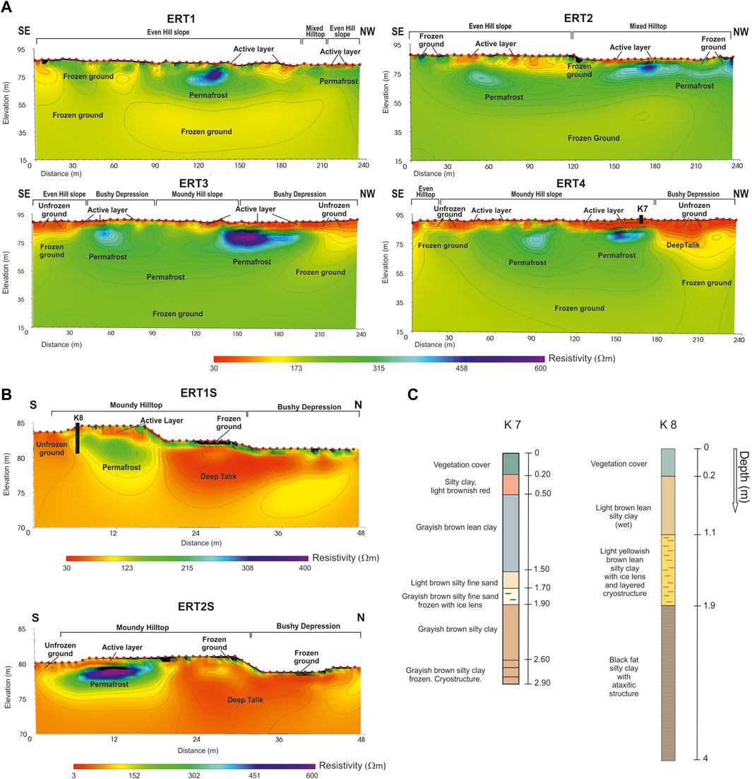
FIGURE 7. ERT sections in (A) Site 1A (ERT1, ERT2, ERT3, and ERT4) and in (B) Site 1B (ERT1S and ERT2S). The positions of boreholes K7 and K8 are indicated on the profiles ERT4 and ERT1S, respectively. The interpretation of the ERT profiles is based on the analyzed resistivity-cryological patterns. ERT sections exhibit a continuous permafrost layer with resistivity values in the range 200 < ρ < 600 Ωm, underlying a low resistivity (ρ < 100 Ωm) active layer. Red dots represent the electrodes deployed along the topographic surface. (C) K7 and K8 borehole stratigraphy (data from Budantseva et al., 2015; Voytenko et al., 2017). The cryolithology highlights the presence of silty clay frozen bodies with cryogenic structures in both boreholes, in agreement with the ERT results. Hence, the silty clay with an ataxitic structure at about 2 m depth in K8 produces the resistivity decrease observed in the ERT1S and ERT2S profiles.

4.3.1 Previous Surveys

The resistivity (ρ) values of the previous geoelectric survey ERT2018 (Figure 6C), acquired in September 2018, are compared with the results obtained from the lithological (Figure 6A) and thermometric (Figure 6B) data at K1, K2, and K3 boreholes. As shown in Figure 1, this profile crosses exactly all three considered boreholes.

As evidenced in the previous section, massive cryostructure and frozen sediments are present at the bottom of K1 and K3 boreholes, as a useful indicator of the permafrost table and of the base of the active layer and unfrozen ground. Comparing the borehole data with the resistivity values of ERT2018 section (Figures 6A–C), it is possible to correlate the active layer base and the permafrost table to resistivity values of approximately 100 and 200 Ωm, respectively. As explained in detail in the Discussion section, the ranges of resistivity values for frozen and unfrozen ground strongly depend on the type of soil. Because clay and silty clay are the dominant sediment type in the study area, these two resistivity thresholds represent the characteristic resistivity values for the active layer base and the permafrost table in the whole area investigated by the geoelectric surveys (Figure 1). Therefore, we based our interpretation of the ERT sections on the following approximate scale of resistivity values: lower than 100 Ωm for the unfrozen ground, active layer, and taliks; ranging between 100 and about 200 Ωm for the frozen ground; and higher than about 200 Ωm for the permafrost. We point out that this resistivity scale is no more valid for other types of soil, characterized by lower clay contents. A similar scale of resistivity has been adopted in other works for this kind of soils (e.g., Vanhala et al., 2010; Isaev V. et al., 2022).

On the basis of this resistivity scale, we interpreted the base of the unfrozen ground and of the active layer along the ERT2018 section (Figure 6C). According to the definition of the active layer, in this interpretation, we indicated as active layer only the parts of the thawed superficial ground underlain by permafrost whereas the other parts were indicated as unfrozen ground. Low-resistivity values are present at shallow depths along the entire profile, in good agreement with the ALT and unfrozen ground thickness (UGT) values in correspondence of boreholes K1 and K3, respectively. The active layer is present in the central and south-eastern parts of the section, it is about 3.5 m thick and exhibits an average resistivity of 40–50 Ωm. The unfrozen ground layer is thicker (about 4.5–5.0 m) and exhibits a lower average resistivity (approximately 20 Ωm) in the south-eastern part of the section, in correspondence of the swamp depression zone. These evidences are in agreement with the temperatures and lithological profile of K3, showing a lower ice content than that of K1.

High-resistivity zones in the ERT section at depths larger than 5 m, with resistivity values up to about 10 kΩm, can be associated with the presence of permafrost. This correlation is in agreement with temperatures below zero and with the presence of massive cryogenic structures at the bottom of the borehole K1. As explained in the Discussion, if clay is predominant also in the deeper parts of the section, the maximum thickness of the permafrost layer should be about 25 m.

As displayed in Figure 6C, the profile shows that the borehole K2 is located in correspondence of a wide and deep low-resistivity body (10 Ωm < ρ < 70 Ωm), showing a 1 m deep topographical depression at the surface (bushy depression landscape microzone, Figure 4). The unusual temperature trend and the lithological profile of K2 indicate the presence of an extensive anomalous unfrozen ground area. Considering the permafrost thickness in this section, this low-resistivity area can be ascribed to a deep talik. Furthermore, two other taliks are probably present between K1 and K3 (ρ < 80 Ωm), corresponding to a swamp depression zone. One of the two taliks is enclosed in frozen ground, whereas the second shows lower average resistivity values, and it is open to the surface. On the basis of our interpretation, the medium around the two taliks shows resistivity values between 100 and 200 Ωm, typical of frozen ground (see also the Discussion) and, most probably, there is no permafrost below them. Therefore, the area including these two taliks can be considered an early-stage deep talik.

This correlation of different types of data from previous surveys enables a better interpretation of the resistivity-cryological patterns on the four new ERT sections acquired in 2019.

4.3.2 Site 1A

The four geoelectric profiles acquired in Site 1A in September 2019, namely, ERT1, ERT2, ERT3, and ERT4, are NW–SE oriented and 30 m spaced to each other (Figure 1). They are located at an average elevation of about 90 m a.s.l. The ground surface topography is characterized by microdepressions of extension ∼1 m², interspersed with hillocks with an elevation difference of about 1 m. On the basis of the resistivity scale adopted for ERT2018, the resulting profiles show the presence of a continuous high-resistivity permafrost layer (200 Ωm < ρ < 600 Ωm) underneath a thin frozen ground layer (100 Ωm < ρ < 200 Ωm) and a low-resistivity (ρ < 100 Ωm) active layer (Figures 7A, 8). As conducted for the ERT2018 profile (see also the Discussion), we interpreted the four sections by adopting a value of 100 Ωm as the characteristic resistivity value of the active layer and unfrozen ground bottom in this area (Figure 8). Also in this case, we indicated as active layer only the parts of the thawed superficial ground underlain by permafrost and as unfrozen ground the other parts. The surveyed area is characterized by an ALT ranging from about 0.5 to 7 m, while the UGT can reach 9 m in some areas.

FIGURE 8

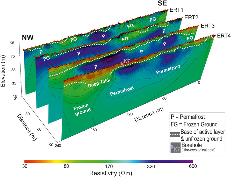
FIGURE 8. 3D representation of the ERT sections in Site 1A. According to the CRIM analysis and to the resistivity-cryological patterns, the interpretation of the active layer and unfrozen ground bottom (white dashed line) is marked by a resistivity value of 100 Ωm. This interpretation, together with the topographic surface (highlighted by red dots representing electrodes deployed during the acquisition), was used to build the ALT and UGT map shown in Figure 9. The talik, permafrost, and frozen and unfrozen ground areas are also highlighted.

The southern part of line ERT1 exhibits a superficial resistive body of about 100–300 Ωm, which denotes discontinuous permafrost and frozen ground. Likewise, the high-resistivity feature at the southern edge of the line ERT2 is characterized by resistivity values similar to those of the permafrost layer. This feature, revealing a frozen ground and massive cryostructure, is located on an even hillslope covered by lichens and small shrubs. Moving northward along the profile, a local thicker (about 4–6 m) low-resistivity active layer (30 Ωm < ρ < 100 Ωm) is present. In the central-northern part of the ERT2, corresponding to a mixed hilltop landscape, covered by lichen on mounds and tall shrubs in the troughs, the ALT becomes thinner, varying between about 0.5 and 2 m.

Lines ERT3 and ERT4 are located on a fairly flat peat surface with few small hollows (1–2 m deep). They exhibit an ALT ranging from 1 to 7 m (an average thickness of about 4 m) with resistivity values ranging from 30 to 100 Ωm. The higher ALT values are present in the NW part of the area, in correspondence of a bushy depression covered by tall birches and shrubs. Borehole K7 is located approximately 5 m on the west with respect to the ERT4 profile. A silty clay frozen body with a cryogenic structure is present at the bottom of this borehole, from 2.6 to 2.9 m depth (Figure 7C). This borehole is not deep enough to reach the base of the active layer, which is about 7 m deep in this position, as inferred from the interpretation of the ERT4 section. However, this profile evidences a high-resistivity (∼100 Ωm) thin lens (∼1 m thick) embedded in the active layer, in agreement with the borehole K7 geocryological core analysis. On the basis of the interpretation of the ERT4 profile, the north-west area shows an extensive low-resistivity unfrozen ground, which is about 16 m thick, underlined by a deep frozen ground body where the permafrost table cannot be detected. This area, characterized by a marshland bushy depression landscape, can be associated with the presence of a deep talik.

The interpretation of the ERT profiles (Figures 7A, 8) enabled us to map the extension and thickness of the unfrozen ground and active layer. However, they contain useful information also about permafrost thickness. These sections show a gradual decrease in the ground resistivity with depth. On the basis of our resistivity scale, if the underground lithology does not vary significantly with depth and clay is predominant (as shown by landscape zonation and borehole stratigraphy), the maximum thickness of the permafrost layer should be about 30 m for ERT1, 40 m for ERT2 and ERT4, and 50 m for ERT3 (Figures 7A, 8). These values are quite in agreement with previous investigations (e.g., Isaev et al., 2020), reporting a permafrost thickness larger than 40 m in this area.

However, as explained in detail in the Discussion, note that the deepest parts of the ERT sections are unreliable because the sensitivity of the geoelectric method decreases with depth. For this reason, in this case, the bottom of the permafrost layer cannot be well defined if its thickness exceeds 50 m.

4.3.3 Site 1B

The two geoelectric profiles ERT1S and ERT2S (Figure 7B), acquired in September 2019, are parallel to each other and located about 30 m west to the Vorkuta River in Site 1B (Figure 1). The landscape is characterized by a 2–2.5 m high (with respect to the average surface elevation of about 81.5 m a.s.l.) moundy hilltop located to the south (with lichens on mounds and tall shrubs in troughs) and a bushy depression covered by tall birches and shrubs located to the north. Rainwater flows south-eastward in the depression and within the valley landscape, draining the surface to the Vorkuta River.

The depression is characterized by low-resistivity (ρ < 100 Ωm, with very low-resistivity values down to about 3 Ωm) sediments covered by a ∼0.5 m thick high-resistivity (100 < ρ < 600 Ωm) superficial layer. Despite the low penetration depth of these two short profiles, this low-resistivity body is probably related to a deep talik area. The K8 borehole (Figure 7C) is located at the moundy hilltop, right on the ERT1S line. Borehole stratigraphy shows a 1.1 m thick wet shallow layer overlying a 0.8 m thick layer with an internal cryostructure, matching quite well the resistivity distribution. Silty clay sediments are predominant also in this area. Permafrost is present below the southern moundy hilltop area, at about 1.5 m depth, and it consists in a 4 m thick high-resistivity layer (200 < ρ < 600 Ωm). In the southern part of both lines, the 1 m thick low-resistivity thawed soil overlying the permafrost is associated with the active layer. Close to the southern edges of profiles ERT1S and ERT2S, resistivity values lower than 100 Ωm indicate the presence of unfrozen ground both in the upper and deeper parts, suggesting that this area could be ascribed to a deep talik as well.

5 Discussion

In the context of accelerating global warming, construction of foundation infrastructures on permafrost requires appropriate methodologies for subsoil characterization (e.g., soil type and petrophysical and mechanical properties). Although the geoelectric technique has been proven an efficient methodology for permafrost characterization, it shows some limitations that can be resumed in these two main points:

• ERT surveys alone are not sufficient to infer the petrophysical properties of the investigated subsoil, namely, the ice content $S_i$, porosity $\Phi$, and clay content $C$. To this aim, it is necessary to integrate ERT data with other geophysical methodologies, for example, the active seismic or GPR methods (e.g., Böhm et al., 2015). Nevertheless, in the absence of other geophysical complementary data, it is possible to estimate some properties using a suitable rock-physics theory and geocryological data describing the type of soil. In the following subsection, we propose a methodology based on the CRIM to analyze how the ice content, clay content, and porosity influence the resistivity of the investigated soils.

• As previously explained, the deepest parts of the ERT sections are generally unreliable because the sensitivity of the geoelectric method decreases with depth. For this reason, often the bottom of the permafrost layer can hardly be resolved. For a homogeneous subsoil, the maximum depth of investigation $z_{max}$ is defined as the depth at which the normalized sensitivity function, integrated with respect to depth, is equal to 1/2 (Edwards, 1977; Szalai et al., 2009). It follows that $z_{max}\approx L/6$ where $L$ is the total array length. In our case, using both the dipole–dipole and pole–dipole arrays, in Site 1A, we have $z_{max}\approx 70$ m.

The results obtained from the ERT2018 profile (calibrated by thermometric and core lithology data) and from the ERT data acquired in 2019 (calibrated by core lithology data) allowed the characterization of the permafrost, frozen ground, and active layer distribution of the Khanovey area near the Vorkuta River. The isopach map shown in Figure 9A has been obtained by interpolating the interpreted ALT and UGT displayed in Figure 8. As previously explained, we indicated as active layer only the parts of the thawed superficial ground underlain by permafrost, and as unfrozen ground the other parts. Figure 9A highlights a gradual increase in ALT moving westward, from ERT1 to ERT4, where it reaches a maximum value of about 7 m, close to the talik. Then, there is an intermediate unfrozen ground zone of thickness ranging from 7 to 9 m around the talik.

FIGURE 9

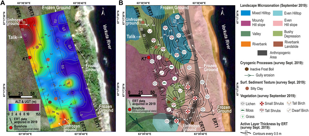
FIGURE 9. (A) ALT and UGT map (contours every 0.5 m) performed from the interpretation of the ERT1, ERT2, ERT3, and ERT4 profiles acquired in Site 1A, superimposed on the satellite image. The map highlights a gradual decrease in ALT by moving eastward to the Vorkuta River; the ALT ranges from 0 m (dark blue) in the eastern side of the map to about 7 m (red) in the NW part. ALT values greater than 7 m represent unfrozen ground areas not underlined by permafrost or an area occupied by a talik. The talik, located in the north-western side of ERT4, exhibits an unfrozen ground thickness up to about 16 m (highlighted in purple). The position of borehole K7 is indicated (red circle). Surface lithology information collected during the geocryological survey is also shown, evidencing that silty clay deposits (brown dots) represent the major soil texture type. (B) ALT isolines (every 0.5 m) superimposed to the landscape microzonation, morphological and cryogenic processes, and vegetation type (2019 field survey). The hilltops are characterized by frozen ground, the hillslopes are characterized by frozen ground to thin/large ALT (1–7 m), and depressions are marked by thick unfrozen ground (7–9 m) or a talik area (9–16 m thick thaw soil in the NW of the map). Local inactive frost boils (dark brown hexagons) are located in correspondence of a 4–5 m ALT, within even hillslope and bushy depression microzone types. The anthropogenic zone (dark gray area) corresponds here to unpaved pathways. Maps compiled using ArcGis^® (Esri) software. Datum: WGS84; projection: UTM 41N. Satellite base image (Gis layer “World Imagery”) retrieved in 2019 from the ArcGis online database resources.

It is possible to correlate those results to geomorphological setting, vegetation, geocryological processes, drainage condition, and landscape zonation, which are strictly related to frozen ground distribution. For instance, the ALT (and UGT) increases in areas such as bushy depressions with tall birches and tall shrubs, whereas hilltops covered by lichens and shrubs are characterized by a shallower permafrost table (Figures 9A, B). The ALT isolines, obtained from the four ERT 2019 profiles, are also shown in Figure 9B, where they are superimposed to the landscape microzonation and geocryological map. The map evidences that silty clay deposits are the major soil type in Site 1A. Moreover, the hilltops are characterized by frozen ground, the hillslopes are characterized by frozen ground to thin/medium ALT (1–7 m), and depressions are marked by thick unfrozen ground (7–9 m) and a deep talik in the NW area. On the basis of our interpretation, the talik is characterized by a 9–16 m thick thawed soil overlying frozen ground. Local inactive frost boils are located in correspondence of a 4–5 m thick active layer, where the permafrost table depth starts increasing westward. Within even hillslope and bushy depression microzone types, the interrupted frost boil due to the increase in the thawed layer allows plants, such as tall birches and tall shrubs, to encroach the area.

Our results showed that permafrost thickness substantially reduces upon approaching the riverbank. A permafrost volume, obtained by a 3D interpolation of the resistivity values higher than 200 Ωm over the four ERT sections of Site 1A, is displayed in Figure 10. This figure clearly shows that the permafrost becomes thinner and discontinuous going eastward. At the same time, Figure 9 shows that the ALT gradually reduces upon approaching the riverbank. This phenomenon is most probably due to the presence of the river. In fact, rivers in permafrost regions can have very significant influence on the thermal state of the nearby permafrost. The thermal impact of warm water and insolation on the riverbank slopes affects the local thermal field and increases the annual temperature of grounds. The difference between the riverbank ground and the internal frozen ground reaches 1°C–2°C for the Vorkuta River zone (Tananaev et al., 2021). The impact area is quite wide, and usually, boreholes are located at least 50 m from the riverbank to avoid this warming effect.

FIGURE 10

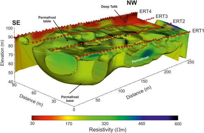
FIGURE 10. Permafrost volume obtained by a 3D interpolation of the resistivity values higher than 200 Ωm over the four ERT sections of Site 1A. Permafrost thickness substantially reduces and becomes discontinuous upon approaching the riverbank.

The fact that the anthropogenic zone of Site 1 is an unpaved footpath means that it does not affect the frozen conditions of the ground, in contrast to the effects of the railway track along which abundant thermokarst lakes are detected (Figures 4, 5A, B).

5.1 Complex Refractive Index Method

The CRIM formula for shaly sandstone with negligible permittivity and partially saturated with groundwater and ice can be expressed as

$\sigma ={\left[\left(1-\Phi \right)\left(1-C\right){\sigma }_q^{\gamma }+\left(1-\Phi \right)C{\sigma }_c^{\gamma }+\Phi S_i{\sigma }_i^{\gamma }+\Phi \left(1-S_i\right){\sigma }_w^{\gamma }\right]}^{1/\gamma }, \gamma =1/2(1)$

(e.g., Schön, 1996; Carcione et al., 2012), where ${\sigma }_q$, ${\sigma }_c$, ${\sigma }_w$, and ${\sigma }_i$ are the sand/silt grain (quartz), clay, groundwater, and ice conductivities and $\sigma$ is the conductivity of the composite medium. Generally, ${\sigma }_i$ depends on temperature and ice impurity content, and ${\sigma }_w$ depends on water salinity. Table 2 shows the typical electrical properties of the different soil components. If γ is a free parameter, Eq. 1 is termed the Lichtnecker–Rother formula. It is based on ray approximation. The travel time in each medium is inversely proportional to the electromagnetic velocity, which, in turn, is inversely proportional to the square root of the complex dielectric constant. At low frequencies, displacement currents can be neglected and the above equation is obtained. For a zero clay content and by neglecting ${\sigma }_q$ and ${\sigma }_i$, Eq. 1 is exactly Archie’s law used in Hoversten et al. (2006).

TABLE 2

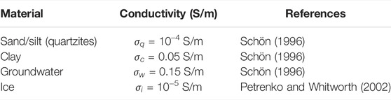
TABLE 2. Typical material electrical properties.

In our case, under realistic assumptions, we can use Eq. 1 to compute the ice content as a function of the porosity, the clay content, and the measured resistivity:

$S_i=\frac{\left(1-\Phi \right)\left(1-C\right){\sigma }_q^{\gamma }+\left(1-\Phi \right)C{\sigma }_c^{\gamma }+\Phi {\sigma }_w^{\gamma }-{\sigma }^{\gamma }}{\Phi ({\sigma }_w^{\gamma }-{\sigma }_i^{\gamma })}, \gamma =1/2(2)$

Figure 11A shows the resistivity values corresponding to permafrost and unfrozen ground, computed using Eq. 1 as a function of porosity $\Phi$ and clay content $C$. The two surfaces represent the resistivity of sediments fully saturated by water ($S_i$ = 0, violet surface) and ice ($S_i$ = 1, cyan surface), respectively. Red and green isolines connect points of equal resistivity on the two surfaces. Moreover, the ice saturation $S_i$, computed using Eq. 2 for different sediment resistivity values, is displayed in Figure 11B. The computation was performed using the MATLAB™ software package.

FIGURE 11

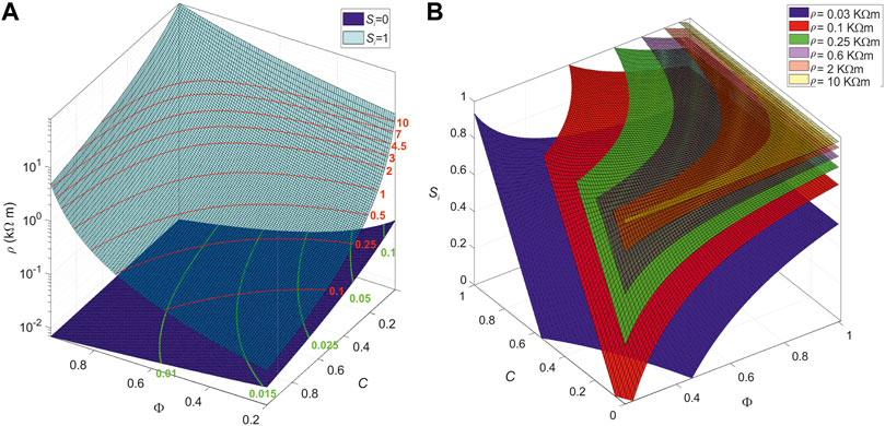
FIGURE 11. Results of the CRIM petrophysical analysis. (A) resistivity of sediments fully saturated by water ($S_i$ = 0, violet surface) and ice ($S_i$ = 1, cyan surface), computed using Eq. 1. Red and green isolines connect points of equal resistivity on the two surfaces. Cyan and violet surfaces correspond to permafrost and unfrozen ground, respectively. (B) ice saturation $S_i$ computed using Eq. 2 for different sediment resistivity. Computation performed by adopting the MATLAB™ software package.

We highlight the following points:

1. The bottom of boreholes K1, K3, and K7 is characterized by the presence of a massive cryostructure and silty clay frozen sediments (Figures 6A, 7C). This means that clay is predominant ($C>$ 0.5) and $S_i\approx$ 1. Moreover, the temperature profile evidences that the bottom of the K1 and K3 boreholes corresponds to the permafrost table and to the unfrozen ground bottom, respectively. The ERT2018 section shows that at the bottom of borehole K1 (Figure 6C), there is a sharp transition of the resistivity from about 100 Ωm (frozen soil) to 200 Ωm (massive cryostructure). This evidence is in agreement with the cyan surface of Figure 11A, where the 100 Ωm isoline indicates the presence of frozen soil with ice content $S_i$ very close to 1 when $C>$ 0.53 and $\Phi <$ 0.55. It is interesting to note that the same isoline on the violet surface may indicate the presence of unfrozen ground for very low clay content and porosity. Therefore, because the results of the landscape zonation showed that the characteristics of the shallow sediments are invariable in correspondence of all ERT profiles (Figure 4), our assumption to consider the resistivity of about 100 Ωm as a marker of the base of the active layer in this area is thus justified.

2. The transition zone from the base of the active layer ($\rho \approx$ 100 Ωm) and the permafrost table ($\rho \approx$ 200 Ωm) is characterized by very high ice saturations (Figure 11B). For example, if we consider a sediment with $\Phi =$ 0.47 and $C=$ 0.58, the ice content can vary from about 0.85 ($\rho =$ 100 Ωm) to 1 ($\rho =$ 200 Ωm).

3. The maximum permafrost resistivity in the ERT sections of Sites 1A and 1B is about 600 Ωm, whereas in ERT2018, it reaches values up to about 10 kΩm (Figures 6C, 7A, B). The cyan surface in Figure 11A shows that this large difference mainly depends on the sediment clay content. In fact, when $\Phi <$ 0.5, a resistivity of 600 Ωm indicates the presence of permafrost with moderate/high clay content ($C>$ 0.3), and a resistivity of 10 kΩm indicates frozen sediments with low clay content (C < 0.1), mainly composed of silt/sand. Therefore, the sediments corresponding to the permafrost layer in the ERT2018 profile probably have a lower clay content in comparison to those of Sites 1A and 1B.

4. Talik and unfrozen ground areas are characterized by minimum resistivity values of 10 Ωm in ERT2018, 30 Ωm in the ERT sections of Sites 1A, and 3 Ωm in the ERT2S section (Figures 6C, 7A, B). The green isolines in Figure 11A indicate that these values strongly depend on the clay content and porosity of unfrozen sediments. A resistivity of 10 Ωm indicates sediments mainly composed of clay with very high porosity ($\Phi \approx$ 0.5). This evidence is confirmed by the K2 stratigraphy, which indicates a massive prevalence of clay and silty clay in the talik. A resistivity of 30 Ωm indicates sediments with $\Phi <$ 0.5 and $C<0.7$. Resistivity values lower than 10 Ωm in the depression of Site 1B are probably due to the presence of fluid (water) flow toward the Vorkuta River.

5. Lithological and geocryological core analysis of boreholes K1 and K7 show that in the active layer there is a coexistence of frozen and unfrozen sediments (Figures 6A, 7C). This evidence produces a strong vertical and horizontal variability of resistivity, from about 30 to 100 Ωm. Ice content $S_i$ strongly depends on $\Phi$ and $C$. For example, Figure 11B shows that for a sediment with $\rho =$ 30 Ωm and $\Phi =$ 0.4, $S_i$ can vary from 0.3 ($C=$ 0.4) to about 0.7 ($C=$ 1). K1 and K7 borehole stratigraphy and landscape microzonation (Figure 4; Table 1) exhibit a predominance of clay in the active layer. If we consider a sediment with $\Phi =$ 0.4 and $C=$ 0.7, the ice content can vary from 0.4 ($\rho =$ 30 Ωm) to about 0.9 ($\rho =$ 100 Ωm). If the clay content is lower, say $C=$ 0.3, the ice content can vary from 0.1 ($\rho =$ 30 Ωm) to 0.6 ($\rho =$ 100 Ωm). Note that for $\Phi <$ 0.5, a sediment with low clay content can be partially saturated with ice and groundwater also when $\rho \ge$ 600 Ωm. For example, the ice content of sand with $\Phi =$ 0.4 can vary from 0.78 ($\rho =$ 600 Ωm) to 0.98 ($\rho =$ 10 kΩm).

6. The ERT sections in Site 1A show a gradual decrease in ground resistivity with depth. As explained in the previous section, if the underground lithology does not vary significantly with depth and clay is predominant (as shown by landscape zonation and borehole stratigraphy), permafrost should also be present in the deeper parts of some sections. Instead, if the clay content decreases significantly with depth, we no longer have permafrost at a certain depth. For example, let us consider profile ERT3, which exhibits an average resistivity of about 250 Ωm at 40 m a.s.l. If $\Phi =$ 0.4 and $C\ge$ 0.35, Figure 11B shows that the pore space is fully saturated by ice and the medium is permafrost. If $C<$ 0.35, there should be also water in the pore space (e.g., with $C=$ 0.2, we have $S_i=$ 0.8) and the medium is no more permafrost.

This discussion shows that the results obtained from the lithological and geocryological core analysis, ERT, landscape microzonation, and ground thermometry are in agreement with each other.

6 Conclusion

Permafrost retreat and degradation are some of the main concerns related to Arctic amplification. Rising temperatures are leading to a gradual deepening of the permafrost table, causing subsidence and a consequent reduction of the ground capacity to carry loads, which leads to the deformation of infrastructures. Investigation and monitoring of permafrost distribution and degradation dynamics are therefore crucial to assess the stability of engineering infrastructures and prevent possible damages.

In this study, we employed geophysical and geocryological methods to characterize the active layer close to a 1.5 km long segment of the Russian North Railway, in the Arctic area of the Khanovey railway station (Komi Republic, Russia). Landscape microzonation, borehole drilling, ground temperature measurements, and geoelectric surveys were carried out. ERT was adopted to invert the geoelectric data and to image the resistivity distribution of the subsurface between the railway and the Vorkuta River. Landscape mapping was performed by satellite image analysis and by collecting field information on geomorphology, vegetation, drainage, cryostructure and lithology, ALT, and soil temperature.

The analysis and integration of different type of data enabled to assess the thawing condition of permafrost in the study area. The correlation of ground temperature and lithological data from three boreholes with a geoelectric profile enabled a better interpretation of the resistivity-cryological patterns. The CRIM was used to integrate and quantitatively validate the results.

Borehole stratigraphy and landscape microzonation indicate a massive prevalence of clay and silty clay at shallow depths. CRIM suggests that the resistivity value of about 100 Ωm can be considered marker of the active layer bottom for this kind of sediments. On the basis of this assumption, the active layer shows a thickness ranging from 0.5 to 7 m and the average ALT is about 4 m. Moreover, in the active layer, there is a coexistence of frozen and unfrozen unconsolidated sediments showing resistivity values ranging from about 30 to 100 Ωm. Here, the ice content estimated using CRIM ranges between about 0.3–04 to 0.9. The underlying permafrost shows resistivity values higher than 200 Ωm. Very high-resistivity values exceeding 600 Ωm and up to 10 kΩm are typical of frozen sediments with massive cryostructure and clay content lower than 30%.

If the underground lithology does not vary significantly with depth and clay is predominant, the maximum thickness of the permafrost layer in the surveyed area should be about 50 m. This thickness, confirmed by previous investigations in this site, gradually reduces and becomes discontinuous upon approaching the riverbank.

The area is characterized by the presence of diffuse thermokarst processes. Open, closed, and deep taliks with resistivity ranging between about 3 and 70 Ωm are scattered in the study area. Taliks are often located in bushy and swamp depressions with birch, shrub, and grass, generally characterized by warmer unfrozen ground. In general, shrubby hillslopes exhibit higher ALT values, and the opposite situation happens in moundy hills mostly covered by lichens.

Thermokarst phenomena develop mainly along the railroad area as a consequence of the thermal regime variation effect due to different factors, e.g., changes in the natural condition of the soil, vegetation removal during railway construction, and the role of railway embankment as a barrier to surface water run-off. Frost heaving is a consequence of the seasonal freezing and thawing of the ground. Thawing permafrost is dangerous because it can trigger thermokarst processes with the consequent development of taliks, which represent a serious hazard for railway embankment stability.

The multidisciplinary approach used in this study, with methods providing investigations at different and complementary resolutions, can also be applied to the western area of Sites 1 and 2, closer to the railway. There, detailed geocryological information and landscape zonation are now available, and therefore, new geophysical acquisition can be planned in order to further investigate the deeper characteristics of the ground. For example, new surveys can be designed to discriminate whether the mapped superficial swamp depressions and thermokarst lakes are underlain by permafrost or represent a shallower expression of a deep talik. This procedure of integration, after an update of any change of landscape and cryological conditions through time, is essential in such geocryologically heterogeneous and complex environment. Moreover, a repetition of the geophysical survey in the same places through the years would enable us to monitor changing conditions in time-lapse. Periodic geocryological and geophysical surveys are therefore required to monitor the rapid evolution of permafrost conditions and to deal with the extreme landscape variability, instability, and heterogeneity of the field area. In this contest, the obtained results will represent valuable information to address the design of engineering solutions and to ensure the structural stability of infrastructures, such as reinforcing the construction foundations and maintaining the thermal balance of the ground. For example, thermosyphons represent a well-established technology, widely used in various Russian permafrost areas to stabilize infrastructures. Another solution could be the diversion of the railroad where the active layer is thinner and the underlying permafrost is thicker and stable.

Data Availability Statement

The datasets presented in this study can be found in online repositories. The names of the repository/repositories and accession number(s) can be found below: https://disk.yandex.ru/d/WOch52cAOx9SHQ?w=1.

Author Contributions

VI conceived this research and, together with AP, EG, DS, and PK, designed and executed the geophysical and geocryological surveys in the Khanovey area. MR participated in the field work, performed large parts of the data processing, and wrote the first draft of the manuscript. MR, MDC, SP, DG, and MG carried out the geophysical data analysis, interpretation, and data integration. MDC and SP contributed to the writing of the manuscript and, together with MLR, supervised the work of MR. All authors contributed to manuscript revision and read and approved the submitted version.

Funding

This research was supported by Norwegian Center for International Cooperation in Education through the “Russian-Norwegian research-based education in cold regions engineering” project (RuNoCORE; CPRU-2017/10015).

Conflict of Interest

The authors declare that the research was conducted in the absence of any commercial or financial relationships that could be construed as a potential conflict of interest.

Publisher’s Note

All claims expressed in this article are solely those of the authors and do not necessarily represent those of their affiliated organizations, or those of the publisher, the editors and the reviewers. Any product that may be evaluated in this article, or claim that may be made by its manufacturer, is not guaranteed or endorsed by the publisher.

Acknowledgments

Special thanks to the Master’s students of Lomonosov Moscow State University, Norwegian University of Science and Technology, and Università degli Studi G. D’Annunzio (Italy) for the assistance in the field activity and to the National Institute of Oceanography and Applied Geophysics—OGS (Italy) for the support in geophysical data analysis. We acknowledge IHS Markit, Geostudi Astier s.r.l., Geotomo Inc., and The MathWorks Inc. for the academic licenses of Kingdom™, ERTLab™—ViewLab3D™, Res2dInv™, and MATLAB™ software packages, respectively. We thank the reviewers, whose constructive comments allowed us to improve the manuscript.

References

Abramov, A., Davydov, S., Ivashchenko, A., Karelin, D., Kholodov, A., Kraev, G., et al. (2019). Two Decades of Active Layer Thickness Monitoring in Northeastern Asia. Polar Geogr. 44, 186–202. doi:10.1080/1088937X.2019.1648581

CrossRef Full Text | Google Scholar

ACGR - Associate Committee on Geotechnical Research (1988). “Glossary of Permafrost and Related Ground-Ice Terms,” in Permafrost Subcommittee, National Research Council of Canada. Editors S. A. Harris, H. M. French, J. A. Heginbottom, G. H. Johnston, B. Ladanyi, D. C. Segoet al.

Google Scholar

Allen, M. R., Dube, O. P., Solecki, W., Aragón-Durand, F., Cramer, W., Humphreys, S., et al. (2018). “Framing and Context,” in Global Warming of 1.5°C. An IPCC Special Report on the Impacts of Global Warming of 1.5°C above Pre-industrial Levels and Related Global Greenhouse Gas Emission Pathways, in the Context of Strengthening the Global Response to the Threat of Climate Change, Sustainable Development, and Efforts to Eradicate Poverty [Masson-Delmotte,. Editors V. P. Zhai, and H. O. Pörtner.

Google Scholar

Anisimov, O., and Reneva, S. (2006). Permafrost and Changing Climate: The Russian Perspective. AMBIO A J. Hum. Environ. 35 (4), 169–175. doi:10.1579/0044-7447(2006)35[169:pacctr]2.0.co;2

CrossRef Full Text | Google Scholar

Arcone, S. A., and Delaney, A. J. (1982). Dielectric Properties of Thawed Active Layers Overlying Permafrost Using Radar at VHF. Radio Sci. 17, 618–626. doi:10.1029/RS017i003p00618

CrossRef Full Text | Google Scholar

Arcone, S. A., Lawson, D. E., Delaney, A. J., Strasser, J. C., and Strasser, J. D. (1998). Ground‐penetratinng Radar Reflection Profiling of Groundwater and Bedrock in an Area of Discontinuous Permafrost. Geophysics 63, 1573–1584. doi:10.1190/1.1444454

CrossRef Full Text | Google Scholar

Biskaborn, B. K., Smith, S. L., Noetzli, J., Matthes, H., Vieira, G., Streletskiy, D. A., et al. (2019). Permafrost Is Warming at a Global Scale. Nat. Commun. 10, 264. doi:10.1038/s41467-018-08240-4

PubMed Abstract | CrossRef Full Text | Google Scholar

Böhm, G., Carcione, J. M., Gei, D., Picotti, S., and Michelini, A. (2015). Cross-Well Seismic and Electromagnetic Tomography for CO₂ Detection and Monitoring in a Saline Aquifer. J. Petroleum Sci. Eng. 133, 245–257. doi:10.1016/j.petrol.2015.06.010

CrossRef Full Text | Google Scholar

Brown, J., Ferrians, O. J, Heginbottom, J. A., and Melnikov, E. S. (1997). Circum-Arctic Map of Permafrost and Ground-Ice Conditions. Washington, DC.

Google Scholar

Brown, J., Ferrians, O., Heginbottom, J. A., and Melnikov, E. (2002). Circum-Arctic Map of Permafrost and Ground-Ice Conditions. Boulder, Colorado USA: Version 2, NSIDC: National Snow and Ice Data Center.

Google Scholar

Brown, J., Hinkel, K. M., and Nelson, F. E. (2000). The Circumpolar Active Layer Monitoring (Calm) Program: Research Designs and Initial Results1. Polar Geogr. 24 (3), 166–258. doi:10.1080/10889370009377698

CrossRef Full Text | Google Scholar

Budantseva, N. A., Gorshkov, E. I., Isaev, V. S., Semenkov, I. N., Usov, A. N., ChizhovaVasil'chuk, Ju. N., et al. (2015). Engineering–geological and Geochemical Features of Palsa and Lithalsa Landscapes in the Area of the “Khanovey” Scientific Educational Facility. Inzh. Geol. 3, 34–50. Available at: https://www.researchgate.net/publication/280943215_ENGINEERING-GEOLOGICAL_AND_GEOCHEMICAL_FEATURES_OF_PALSA_AND_LITHALSA_LANDSCAPES_IN_THE_AREA_OF_THE_KHANOVEY_SCIENCE_EDUCATION_STATION

Google Scholar

Buldovicz, S. N., Khilimonyuk, V. Z., Bychkov, A. Y., Ospennikov, E. N., Vorobyev, S. A., Gunar, A. Y., et al. (2018). Cryovolcanism on the Earth: Origin of a Spectacular Crater in the Yamal Peninsula (Russia). Sci. Rep. 8, 13534. doi:10.1038/s41598-018-31858-9

PubMed Abstract | CrossRef Full Text | Google Scholar

Carcione, J. M., Gei, D., Picotti, S., and Michelini, A. (2012). Cross-Hole Electromagnetic and Seismic Modeling for CO₂ Detection and Monitoring in a Saline Aquifer. J. Petroleum Sci. Eng. 100, 162–172. doi:10.1016/j.petrol.2012.03.018

CrossRef Full Text | Google Scholar

Carcione, J. M., and Seriani, G. (1998). Seismic and Ultrasonic Velocities in Permafrost. Geophys. Prospect. 46 (4), 441–454. doi:10.1046/j.1365-2478.1998.1000333.x

CrossRef Full Text | Google Scholar

Chen, T., Ma, W., Wu, Z.-J., and Mu, Y.-h. (2014). Characteristics of Dynamic Response of the Active Layer Beneath Embankment in Permafrost Regions along the Qinghai-Tibet Railroad. Cold Regions Sci. Technol. 98, 1–7. doi:10.1016/j.coldregions.2013.10.004

CrossRef Full Text | Google Scholar

Delaney, A. J., Arcone, S. A., and Chacho, E. F. (1990). Winter Short-Pulse Studies on the Tanana River, Alaska. Arctic 43, 244–250. doi:10.14430/arctic1618

CrossRef Full Text | Google Scholar

Doolittle, J. A., Hardisky, M. A., and Gross, M. F. (1990). A Ground-Penetrating Radar Study of Active Layer Thicknesses in Areas of Moist Sedge and Wet Sedge Tundra Near Bethel, Alaska, U.S.A. Arct. Alp. Res. 22 (2), 175–182. doi:10.1080/00040851.1990.12002779

CrossRef Full Text | Google Scholar

Drozdov, D., Rumyantseva, Y., Malkova, G., Romanovsky, V., Abramov, A., Konstantinov, P., et al. (2015). “Monitoring of Permafrost in Russia and the International GTN-P Project,” in 68th Canadian Geotechnical Conf. GEOQuébec 2015. paper 617.

Google Scholar

Duguay, C. R., Green, J., and Derksen, C.English (2005). “Preliminary Assessmentof the Impact of Lakes on Passive Microwave Snow Retrieval Algorithms in the Arc-Tic,” in Proceedings of 62nd Eastern Snow Conference (Canada: Waterloo, Ontario), 223–228.

Google Scholar

Edwards, L. S. (1977). A Modified Pseudosection for Resistivity and IP. Geophysics 42 (5), 1020–1036. doi:10.1190/1.1440762

CrossRef Full Text | Google Scholar

EEA - European Environment Agency (2017). The Arctic Environment - European Perspectives on a Changing Arctic. Luxembourg: Publications Office of the European Union.

Google Scholar

Farzamian, M., Vieira, G., Monteiro Santos, F. A., Yaghoobi Tabar, B., Hauck, C., Paz, M. C., et al. (2020). Detailed Detection of Active Layer Freeze-Thaw Dynamics Using Quasi-Continuous Electrical Resistivity Tomography (Deception Island, Antarctica). Cryosphere 14, 1105–1120. doi:10.5194/tc-14-1105-2020

CrossRef Full Text | Google Scholar

Folk, R. L. (1954). The Distinction between Grain Size and Mineral Composition in Sedimentary-Rock Nomenclature. J. Geol. 62, 344–359. doi:10.1086/626171

CrossRef Full Text | Google Scholar

Francese, R. G., Bondesan, A., Giorgi, M., Picotti, S., Carcione, J., Salvatore, M. C., et al. (2019). Geophysical Signature of a World War I Tunnel-like Anomaly in the Forni Glacier (Punta Linke, Italian Alps). J. Glaciol. 65, 798–812. doi:10.1017/jog.2019.59

CrossRef Full Text | Google Scholar

Goryachkin, S. V., Zlotin, R. I., and Tertitsky, G. M. (1994). “Russian-Swedish Expedition,” in Tundra Ecology-94": Diversity of Natural Ecosystems in the Russian Arctic (A guidebook).

Google Scholar

Gruber, S. (2012). Derivation and Analysis of a High-Resolution Estimate of Global Permafrost Zonation. Cryosphere 6, 221–233. doi:10.5194/tc-6-221-2012

CrossRef Full Text | Google Scholar

Gilbert, G., Instanes, A., Instanes, A., Sinitsyn, A., and Aalberg, A. (2019). Characterization of Two Sites for Geotechnical Testing in Permafrost: Longyearbyen, Svalbard. AIMS Geosci. 5 (4), 868–885. doi:10.3934/geosci.2019.4.868

CrossRef Full Text | Google Scholar

Harris, S. A., Brouchkov, A., and Guodong, C. (2017). Geocryology: Characteristics and Use of Frozen Ground and Permafrost Landforms. 1st Edition. London: CRC Press, 810. doi:10.4324/9781315166988

CrossRef Full Text

Hinkel, K. M., Doolittle, J. A., Bockheim, J. G., Nelson, F. E., Paetzold, R., Kimble, J. M., et al. (2001). Detection of Subsurface Permafrost Features with Ground-Penetrating Radar, Barrow, Alaska. Permafr. Periglac. Process. 12, 179–190. doi:10.1002/ppp.369

CrossRef Full Text | Google Scholar

Hinkel, K. M., and Nicholas, J. R. J. (1995). Active Layer Thaw Rate at a Boreal Forest Site in Central Alaska, U.S.A. Arct. Alp. Res. 27 (1), 72–80. doi:10.1080/00040851.1995.1200309810.2307/1552069

CrossRef Full Text | Google Scholar

Hinkel, K. M., and Nelson, F. E. (2003). Spatial and Temporal Patterns of Active Layer Thickness at Circumpolar Active Layer Monitoring (Calm) Sites in Northern Alaska, 1995–2000. J. Geophys. Res. 108 (D2), 8168. doi:10.1029/2001JD000927

CrossRef Full Text | Google Scholar

Hinzman, L. D., Goering, D. J., and Kane, D. L. (1998). A Distributed Thermal Model for Calculating Soil Temperature Profiles and Depth of Thaw in Permafrost Regions. J. Geophys. Res. 103 (D22), 28975–28991. doi:10.1029/98JD01731

CrossRef Full Text | Google Scholar

Hjort, J., Streletskiy, D., Doré, G., Wu, Q., Bjella, K., and Luoto, M. (2022). Impacts of Permafrost Degradation on Infrastructure. Nat. Rev. Earth Environ. 3 (1), 24–38. doi:10.1038/s43017-021-00247-8

CrossRef Full Text | Google Scholar

Hong, E., Perkins, R., and Trainor, S. (2014). Thaw Settlement Hazard of Permafrost Related to Climate Warming in Alaska. Arctic 67 (1), 93–103. doi:10.14430/arctic4368

CrossRef Full Text | Google Scholar

Hoversten, G. M., Cassassuce, F., Gasperikova, E., Newman, G. A., Chen, J., Rubin, Y., et al. (2006). Direct Reservoir Parameter Estimation Using Joint Inversion of Marine Seismic AVA and CSEM Data. Geophysics 71, C1–C13. doi:10.1190/1.2194510

CrossRef Full Text | Google Scholar

IPCC (2017). “Report of the Intergovernmental Panel on Climate Change Expert Meeting on Mitigation, Sustainability and Climate Stabilization Scenarios,” in IPCC Working Group III Technical Support Unit. Editors P. R. Shukla, J. Skea, R. Diemen, E. Huntley, M. Pathak, J. Portugal Pereiraet al. (London, UK: Imperial College London), 44.

Google Scholar

Isaev, V. S., Kotov, P. I., and Khilimonjuk, V. Z. (2022). “Manual for Vorkuta Fieldwork Activities,”. Editors P. I. Kotov, and G. I. Gordeeva (Moscow, Russia: KDU), 200.

Google Scholar

Isaev, V., Kioka, A., Kotov, P., Sergeev, D. O., Uvarova, A., Koshurnikov, A., et al. (2022). Multi-parameter Protocol for Geocryological Test Site: A Case Study Applied for the European North of Russia. Energies 15 (6), 2076. doi:10.3390/en15062076

CrossRef Full Text | Google Scholar

Isaev, V., Kotov, P., and Sergeev, D. (2020). “Technogenic Hazards of Russian North Railway,” in Transportation Soil Engineering in Cold Regions. Lecture Notes in Civil Engineering. Editors A. Petriaev, and A. Konon (Singapore: Springer), Vol. 1, 311–320.

Google Scholar

Isaev, V. S., Tyurin, A. I., Sergeev, D. O., Gorshkov, Е. I., Volkov, N. G., and Stefanov, S. M. (2016). The Day of Science and Innovation: New Methods and Ways of Field Geocryological Researches. Vestn. Mosk. Univ. Seriâ 4, Geol. 1, 98–102. doi:10.33623/0579-9406-2016-1-98-102

CrossRef Full Text | Google Scholar

Jensen, J. R. (2007). Remote Sensing of the Environment: An Earth Resource Perspective. Harlow: Brigham Young University. Pearson College Div.

Google Scholar

Jorgenson, M. T. (2022). “Thermokarst,” in Treatise on Geomorphology. Editor J. F. Shroder. Second Edition (Academic Press), 4, 392–414. doi:10.1016/b978-0-12-818234-5.00058-4

CrossRef Full Text | Google Scholar

Kasprzak, M. (2015). High-resolution Electrical Resistivity Tomography Applied to Patterned Ground, Wedel Jarlsberg Land, South-West Spitsbergen. Polar Res. 34, 25678. doi:10.3402/polar.v34.25678

CrossRef Full Text | Google Scholar

Kasprzak, M., Strzelecki, M. C., Traczyk, A., Kondracka, M., Lim, M., and Migała, K. (2017). On the Potential for a Bottom Active Layer Below Coastal Permafrost: the Impact of Seawater on Permafrost Degradation Imaged by Electrical Resistivity Tomography (Hornsund, SW Spitsbergen). Geomorphology 293, 347–359. doi:10.1016/j.geomorph.2016.06.013

CrossRef Full Text | Google Scholar

Kaverin, D., Malkova, G., Zamolodchikov, D., Shiklomanov, N., Pastukhov, A., Novakovskiy, A., et al. (2021). Long-Term Active Layer Monitoring at CALM Sites in the Russian European North. Polar Geogr. 44 (3), 203–216. doi:10.1080/1088937X.2021.1981476

CrossRef Full Text | Google Scholar

Kim, Y., Kimball, J. S., McDonald, K. C., and Glassy, J. (2011). Developing a Global Data Record of Daily Landscape Freeze/thaw Status Using Satellite Passive Microwave Remote Sensing. IEEE Trans. Geosci. Remote Sens. 49 (3), 949–960. doi:10.1109/TGRS.2010.2070515

CrossRef Full Text | Google Scholar

Kimball, J. S., McDonald, K. C., Running, S. W., and Frolking, S. E. (2004). Satellite Radar Remote Sensing of Seasonal Growing Seasons for Boreal and Subalpine Evergreen Forests. Remote Sens. Environ. 90, 243–258. doi:10.1016/j.rse.2004.01.002

CrossRef Full Text | Google Scholar

Klimenko, S. S., Anischenko, L. A., and Antoshkina, A. I. (2011). Chapter 13 The Timan–Pechora Sedimentary Basin: Palaeozoic Reef Formations and Petroleum Systems. Geol. Soc. 35, 223–236. doi:10.1144/M35.13

CrossRef Full Text | Google Scholar

Léger, E., Dafflon, B., Soom, F., Peterson, J., Ulrich, C., and Hubbard, S. (2017). Quantification of Arctic Soil and Permafrost Properties Using Ground-Penetrating Radar and Electrical Resistivity Tomography Datasets. IEEE J. Sel. Top. Appl. Earth Obs. Remote Sens. 10 (10), 4348–4359. doi:10.1109/JSTARS.2017.2694447

CrossRef Full Text | Google Scholar

Marohasy, J. (2017). Climate Change: The Facts 2017. With the Contribution of: John Abbot, Sallie Baliunas, Simon Breheny, Paul Driessen, Tony Heller, Craig Idso, Clive James, Bjørn Lomborg, Pat Michaels, John Nicol, Jo Nova, Ian Plimer, Tom Quirk, Peter Ridd, Matt Ridley, Ken Ring, John Roskam, Nicola Scafetta, Willie Soon, Roy Spencer, Jaco Vlok, Anthony Watts. Redland Bay, Ql: Connor Court Publishing, 380.

Google Scholar

Maslakov, A., Shabanova, N., Zamolodchikov, D., Volobuev, V., and Kraev, G. (2019). Permafrost Degradation within Eastern Chukotka CALM Sites in the 21st Century Based on CMIP5 Climate Models. Geosciences 9, 232. doi:10.3390/geosciences9050232

CrossRef Full Text | Google Scholar

Melnikov, V. P., Osipov, V. I., Brouchkov, A. V., Falaleeva, A. A., Badina, S. V., Zheleznyak, M. N., et al. (2022). Climate Warming and Permafrost Thaw in the Russian Arctic: Potential Economic Impacts on Public Infrastructure by 2050. Nat. Hazards 112, 231–251. doi:10.1007/s11069-021-05179-6

CrossRef Full Text | Google Scholar

Nelson, F. E., Shiklomanov, N. I., Mueller, G. R., Hinkel, K. M., Walker, D. A., and Bockheim, J. G. (1997). Estimating Active-Layer Thickness over a Large Region: Kuparuk River Basin, Alaska, U.S.A. Arct. Alp. Res. 29 (4), 367–378. doi:10.2307/1551985

CrossRef Full Text | Google Scholar

Nelson, F. E., Shiklomanov, N. I., and Mueller, G. R. (1999). Variability of Active-Layer Thickness at Multiple Spatial Scales, North-central Alaska, U.S.A. Arct. Antarct. Alp. Res. 31 (2), 179–186. doi:10.1080/15230430.1999.12003295

CrossRef Full Text | Google Scholar

NOAA/NASA (2020). Annual Global Analysis for 2019. Global Report. Available at: https://www.ncdc.noaa.gov/sotc/global/201913.

Google Scholar

NSIDC - National Snow and Ice Data Center (2020). Advancing Knowledge of Earth's Frozen Regions. Cryosphere Glossary. Available at: https://nsidc.org/cryosphere/glossary.

Google Scholar

Oelke, C., Zhang, T., Serreze, M. C., and Armstrong, R. L. (2003). Regional-scale Modeling of Soil Freeze/thaw over the Arctic Drainage Basin. J. Geophys. Res. 108 (D10), 4314. doi:10.1029/2002JD002722

CrossRef Full Text | Google Scholar

Osterkamp, T. E., and Burn, C. R. (2003). “Permafrost,” in Encyclopedia of Atmospheric Sciences. Editors J. R. Holton, J. Pyle, and J. A. Curry (Oxford: Academic Press), 1717–1729. doi:10.1016/B0-12-227090-8/00311-0

CrossRef Full Text | Google Scholar

Palacky, G. J. (1988). “Resistivity Characteristics of Geologic Targets,” in Electromagnetic Methods in Applied Geophysics. Editor M. N. Nabighian (Tulsa, Oklahoma: Society of Exploration Geophysicists), 53–129.

Google Scholar

Park, H., Kim, Y., and Kimball, J. S. (2016). Widespread Permafrost Vulnerability and Soil Active Layer Increases over the High Northern Latitudes Inferred from Satellite Remote Sensing and Process Model Assessments. Remote Sens. Environ. 175, 349–358. doi:10.1016/j.rse.2015.12.046

CrossRef Full Text | Google Scholar

Peng, X., Zhang, T., Cao, B., Wang, Q., Wang, K., Shao, W., et al. (2016). Changes in Freezing-Thawing Index and Soil Freeze Depth over the Heihe River Basin, Western China. Arct. Antarct. Alp. Res. 48, 161–176. doi:10.1657/AAAR00C-13-127

CrossRef Full Text | Google Scholar

Petrenko, V. F., and Whitworth, R. W. (2002). Physics of Ice. New York: Oxford University Press, 373.

Google Scholar

Picotti, S., Francese, R., Giorgi, M., Pettenati, F., and Carcione, J. M. (2017). Estimation of Glacier Thicknesses and Basal Properties Using the Horizontal-To-Vertical Component Spectral Ratio (HVSR) Technique from Passive Seismic Data. J. Glaciol. 63, 229–248. doi:10.1017/jog.2016.135

CrossRef Full Text | Google Scholar

Romanovsky, V. E., Smith, S. L., Isaksen, K., Shiklomanov, N. I., Streletskiy, D. A., Kholodov, A. L., et al. (2018). Terrestrial Permafrost. In ‘State of the Climate in 2017. Bull. Am. Meteorol. Soc. 99, 161–165. doi:10.1175/2018BAMSStateoftheClimate.1

CrossRef Full Text | Google Scholar

Romanovsky, V. E., Drozdov, D. S., Oberman, N. G., Malkova, G. V., Kholodov, A. L., Marchenko, S. S., et al. (2010). Thermal State of Permafrost in Russia. Permafr. Periglac. Process. 21, 136–155. doi:10.1002/ppp.683

CrossRef Full Text | Google Scholar

Sazonova, T. S., and Romanovsky, V. E. (2003). A Model for Regional-Scale Estimation of Temporal and Spatial Variability of Active Layer Thickness and Mean Annual Ground Temperatures. Permafr. Periglac. Process. 14, 125–139. doi:10.1002/ppp.449

CrossRef Full Text | Google Scholar

Schneider von Deimling, T., Lee, H., Ingeman-Nielsen, T., Westermann, S., Romanovsky, V., Lamoureux, S., et al. (2021). Consequences of Permafrost Degradation for Arctic Infrastructure - Bridging the Model Gap between Regional and Engineering Scales. Cryosphere 15, 2451–2471. doi:10.5194/tc-15-2451-2021

CrossRef Full Text | Google Scholar

Schön, J. H. (1996). Physical Properties of Rocks. Handbook of Geophysical Exploration. Oxford: Pergamon Press.

Google Scholar

Schwamborn, G., Heinzel, J., and Schirrmeister, L. (2008). Internal Characteristics of Ice-Marginal Sediments Deduced from Georadar Profiling and Sediment Properties (Brøgger Peninsula, Svalbard). Geomorphology 95, 74–83. doi:10.1016/j.geomorph.2006.07.032

CrossRef Full Text | Google Scholar

Seppi, R., Zanoner, T., Carton, A., Bondesan, A., Francese, R., Carturan, L., et al. (2015). Current Transition from Glacial to Periglacial Processes in the Dolomites (South-Eastern Alps). Geomorphology 228, 71–86. doi:10.1016/j.geomorph.2014.08.025

CrossRef Full Text | Google Scholar

Sinitsyn, A. O., Guegan, E., Shabanova, N., Kokin, O., and Ogorodov, S. (2020). Fifty Four Years of Coastal Erosion and Hydrometeorological Parameters in the Varandey Region, Barents Sea. Coast. Eng. 157, 103610. doi:10.1016/j.coastaleng.2019.103610

CrossRef Full Text | Google Scholar

Streletskiy, D., Anisimov, O., and Vasiliev, A. (2015). “Chapter 10 - Permafrost Degradation,” in Snow and Ice-Related Hazards, Risks and Disasters. Editor A. Vasiliev (Elsevier), 303–344. doi:10.1016/B978-0-12-394849-6.00010-X

CrossRef Full Text | Google Scholar

Streletskiy, D. A., Suter, L. J., Shiklomanov, N. I., Porfiriev, B. N., and Eliseev, D. O. (2019). Assessment of Climate Change Impacts on Buildings, Structures and Infrastructure in the Russian Regions on Permafrost. Environ. Res. Lett. 14, 025003. doi:10.1088/1748-9326/aaf5e6

CrossRef Full Text | Google Scholar

Streletskiy, D., and Shiklomanov, N. (2016). “Russian Arctic Cities through the Prism of Permafrost,” in Sustaining Russia’s Arctic Cities: Resource Politics, Migration, and Climate Change. Editor R. W. Orttung (Berghahn Press), 201–220. doi:10.2307/j.ctvswx6s0.14

CrossRef Full Text | Google Scholar

Szalai, S., Novák, A., and Szarka, L. (2009). Depth of Investigation and Vertical Resolution of Surface Geoelectric Arrays. J. Environ. Engg. Geophys. 14, 15–23. doi:10.2113/JEEG14.1.15

CrossRef Full Text | Google Scholar

Tananaev, N., Isaev, V., Sergeev, D., Kotov, P., and Komarov, O. (2021). Hydrological Connectivity in a Permafrost Tundra Landscape Near Vorkuta, North-European Arctic Russia. Hydrology 8 (3), 106. doi:10.3390/hydrology8030106

CrossRef Full Text | Google Scholar

Thomson, L. I., Osinski, G. R., and Pollard, W. H. (2012). The Dielectric Permittivity of Terrestrial Ground Ice Formations: Considerations for Planetary Exploration Using Ground-Penetrating Radar. J. Geophys. Res. 117, n–a. doi:10.1029/2012JE004053

CrossRef Full Text | Google Scholar

Tyurin, A. I., Isaev, V. S., Sergeev, D. O., Tumskoi, V. E., Volkov, N. G., Sokolov, I. S., et al. (2019). Improvement of Field Methods for Engineering Geocryological Surveying. Mosc. Univ. Geol. Bull. 74, 297–309. doi:10.3103/S014587521903013X

CrossRef Full Text | Google Scholar

Ulyanov, V. Y. (2021). Ways to Increase the Efficiency of Thermopressiometry. Vìsn. Dnìpropetr. Nac. Unìv. zalìzničnogo Transp. Ìm. Akad. V. Lazarâna 2 (92), 84–91. doi:10.15802/stp2021/237279

CrossRef Full Text | Google Scholar

USSR Engineering Geology(1991). Platform Regions of the European Part of the USSR. Book 2. Moscow: Nedra.

Google Scholar

Vanhala, H., Lintinen, P., Oberman, N., and Jokinen, J. (2010). “Monitoring Permafrost Degradation with Geophysical Methods,” in Report of Year 2009 Studies by the River Ko-Rotaikha, NW Russia (Geological survey of Finland Report, Finland).

Google Scholar

Vasiliev, A. A., Drozdov, D. S., Gravis, A. G., Malkova, G. V., Nyland, K. E., and Streletskiy, D. A. (2020). Permafrost Degradation in the Western Russian Arctic. Environ. Res. Lett. 15, 045001. doi:10.1088/1748-9326/ab6f12

CrossRef Full Text | Google Scholar

Voytenko, A. S., Grishakina, E. A., Grishakina, E. A., Isayev, V. S., Koshurnikov, A. V., Pogorelov, A. A., et al. (2017). Importance of Permafrost Changes for Infrastructure Exploitation and Environmental Protection (Case Study of Local Investigation in Lower Part of Vorkuta River). Arctic: Ecol.Econ. 2 (26), 53–61. doi:10.25283/2223-4594-2017-2-53-61

CrossRef Full Text | Google Scholar

Voytenko, A. S., and Sergeev, D. O. (2016). “Cumulative Economic Damages in Permafrost Based on an Example of a Linear Infrastructure (Railway Khanovey – Pesets),” in Proceedings of the XI International Conference on Permafrost. Editors F. Günther, and A. M. Potsdam.

Google Scholar

Wagner, A. M., Lindsey, N. J., Dou, S., Gelvin, A., Saari, S., Williams, C., et al. (2018). Permafrost Degradation and Subsidence Observations during a Controlled Warming Experiment. Sci. Rep. 8 (1), 10908. doi:10.1038/s41598-018-29292-y

PubMed Abstract | CrossRef Full Text | Google Scholar

Wagner, A. M. (2014). Review of Thermosyphon Applications. Hanover, New Hampshire: Cold Regions Research and Engineering Laboratory, US Army Engineer Research and Development Center. ERDC/CRREL TR-14-1.

Google Scholar

Wang, C., Wang, Z., Kong, Y., Zhang, F., Yang, K., and Zhang, T. (2019). Most of the Northern Hemisphere Permafrost Remains under Climate Change. Sci. Rep. 9, 3295. doi:10.1038/s41598-019-39942-4

PubMed Abstract | CrossRef Full Text | Google Scholar

Yang, Z.-p., Ou, Y. H., Xu, X.-l., Zhao, L., Song, M.-h., and Zhou, C.-p. (2010). Effects of Permafrost Degradation on Ecosystems. Acta Ecol. Sin. 30 (1), 33–39. doi:10.1016/j.chnaes.2009.12.006

CrossRef Full Text | Google Scholar

Yershov, E. D. (1998). General Geocryology. Studies in Polar Research Series. First Published in Russian as Obshchaya Geokriologiya by Nedra, 1990. Xxiii + 580 Pp. Cambridge. New York, Melbourne: Cambridge University Press.

Google Scholar

Yi, Y., and Kimball, J. S. (2020). ABoVE: Active Layer Thickness from Remote Sensing Permafrost Model, Alaska, 2001-2015. Oak Ridge, Tennessee, USA: ORNL DAAC.

Google Scholar

You, Y., Wang, J., Wu, Q., Yu, Q., Pan, X., Wang, X., et al. (2017). Causes of Pile Foundation Failure in Permafrost Regions: The Case Study of a Dry Bridge of the Qinghai-Tibet Railway. Eng. Geol. 230, 95–103. doi:10.1016/j.enggeo.2017.10.004

CrossRef Full Text | Google Scholar

Zhang, T., Barry, R. G., and Armstrong, R. L. (2004). Application of Satellite Remote Sensing Techniques to Frozen Ground Studies. Polar Geogr. 28, 163–196. doi:10.1080/789610186

CrossRef Full Text | Google Scholar

Zhang, T., Barry, R. G., Knowles, K., Heginbottom, J. A., and Brown, J. (2008). Statistics and Characteristics of Permafrost and Ground-Ice Distribution in the Northern Hemisphere. Polar Geogr. 31 (2), 47–68. doi:10.1080/10889370802175895

CrossRef Full Text | Google Scholar