 Cuihui Xia
 Tandong Yao1,3
- 1Big Science Program Center, Institute of Tibetan Plateau Research, Chinese Academy of Sciences, Beijing, China
- 2University of Chinese Academy of Sciences, Beijing, China
- 3Key Laboratory of Tibetan Environment Changes and Land Surface Processes, Institute of Tibetan Plateau Research, Chinese Academy of Sciences, Beijing, China
- 4Tencent AI Platform Department, Shenzhen, China
- 5National Climate Center, China Meteorological Administration, Beijing, China
Extreme weather induced by climate change has triggered large-scale power outages worldwide, particularly during the cold season. More insight into the climatic impacts (especially those of precipitation) on cold season residential electricity consumption (REC) is needed. This study quantified the climatic impacts on REC, with a focus on precipitation, and projected the associated changes under representative concentration pathways (RCPs) 2.6, 4.5, and 8.5 climate change scenarios in Lanzhou and Lhasa, two cities in China with distinctive cold season climates. The climatic impacts on REC in both cities are driven by heating-related demand. A stronger precipitation impact during the cold season was observed in both cities, since precipitation (particularly snowfall) boosts electricity consumption during the cold season. As the two cities become warmer and wetter, increased precipitation will offset the impact of warming on REC, with Lanzhou being more strongly affected. Based on the projections for Lanzhou, the offsetting effect will be more pronounced during the cold season across all scenarios, and will be particularly strong under RCP 2.6. For the remainder of the year, the effects of increased precipitation and warming will have competing importances under the RCP 4.5 scenario, whereas temperature effects will generally dominate the climatic impacts under the RCP 8.5 scenario. These results provide new insights for future cold season climate–energy studies and can be used to improve regional climate adaptation policies. We also propose a method to project climate-based REC changes which is compatible with potential early-warning projects to protect against extreme weather-induced power outages.
1 Introduction
Extreme weather events induced by climate change threaten energy supplies worldwide (Mideksa and Kallbekken, 2010). This threat is particularly pronounced during the cold season. The Hunan power shortage in China in 2020 (Zheng, 2020), the Texas power crisis in the United States in 2021 (Busby et al., 2021), as well as the power outages in the northeastern United States in 2022 (Aljazeera, 2022) all occurred during the cold season. Understanding how residential electricity consumption (REC) responds to climatic conditions during the cold season is critical for mitigating these threats, and can assist in evaluating the social cost of carbon, which is a key indicator for policies focused on mitigating climate change (Nordhaus, 2017; Li et al., 2019), and developing targeted adaptive measures (Deschênes and Greenstone, 2011; Auffhammer and Mansur, 2014; Davis and Gertler, 2015; Auffhammer et al., 2017).
Previous studies have suggested that the climatic impacts on REC are mostly due to heating and cooling demands, and that climate change will increase and decrease REC during the warm and cold seasons, respectively (Deschênes and Greenstone, 2011; Auffhammer and Mansur, 2014; Auffhammer et al., 2017; Waite et al., 2017). In Earth science, climate is defined as the mean temperature and precipitation, and their seasonal variations over time (Strahler, 2011). Climate change not only increases summer temperatures, but can also affect precipitation and induce more extreme weather throughout the year (Cohen et al., 2014). The power outage events mentioned above were all accompanied by snowfall/blizzard events, indicating that the role of precipitation (particularly snowfall) is critical for estimating heating-related REC during the cold season.
Compared to temperature, precipitation has been largely generalized in the econometric models used in previous studies (Davis and Gertler, 2015; Auffhammer et al., 2017; Li et al., 2019; Du et al., 2020; Zhang et al., 2020). Cooling degree days (CDD) and heating degree days (HDD) are used to group temperature data (Du et al., 2020; Zhang et al., 2020). However, there is no equivalent metric for precipitation data. Another method for sorting temperature data uses distribution-based temperature bins (Deschênes and Greenstone, 2011; Davis and Gertler, 2015; Li et al., 2019); however, fewer data points are available for precipitation than temperature during a given study period (Deschênes and Greenstone, 2011; Davis and Gertler, 2015). Alternatively, precipitation can be treated as a covariate or control variable, i.e., as the background setting rather than the focus of the study (Auffhammer et al., 2017; Zhang et al., 2020), which effectively attributes less attention to precipitation than to temperature. However, precipitation does affect REC (Auffhammer and Aroonruengsawat, 2011; Deschênes and Greenstone, 2011), and precipitation changes have been shown to increase the predictive uncertainty of REC in Jiangsu, an eastern province of China (Zhang et al., 2020). Moreover, precipitation has been found to be playing a key role in shaping cold-season REC (Xia et al., 2022).
This study aimed to quantify the impacts of climate on REC and project future trends under climate change in two cities with distinctive cold season climates, with a particular focus on how future precipitation changes will impact REC. This study hypothesized that precipitation impacts heating-related REC during the cold season, likely in the form of snowfall. If this hypothesis is correct, climatic impacts on REC during the cold season may not simply decrease with climatic warming, but instead may increase if there more precipitation occurs during the cold season. To test this hypothesis, an algorithm model was constructed using seven machine learning algorithms and predicted the future climatic impacts on REC under three climate scenarios projected with different greenhouse gas representative concentration pathways (RCPs). The RCPs used herein were: RCP 2.6, in which greenhouse gas emissions are expected to begin decreasing by 2020 and reach zero by 2,100; RCP 4.5, in which emissions are assumed to peak around 2040 and then decline; and RCP 8.5, in which emissions continue to increase throughout the 21st century.
Two cities in China, Lanzhou and Lhasa, were selected as the research targets. These two cities were selected to represent different climate patterns. As indicated by Figure 1, the region where Lanzhou and Lhasa are located is generally cold due to the uplift of the Tibetan Plateau, and climate in the region is greatly shaped by atmospheric circulations of westerlies and monsoons; Lanzhou is located in the prevailing westerly-dominated climate zone, while Lhasa is located in the monsoon-dominated climate zone (Yao et al., 2013). Lanzhou has a longer cold season (hereinafter defined as months with average temperatures below 0 °C) than Lhasa. Lanzhou also receives more precipitation during the cold season than Lhasa, where precipitation events are concentrated in the warm season (Yao et al., 2013). These two cities also represent the different heating infrastructures present in northern and southern China, as defined by the Qinling–Huaihe Line. Lanzhou is equipped with a central coal-fueled heating system, as in other northern cities, while Lhasa relies mostly on household electric heating, as does the rest of southern China.
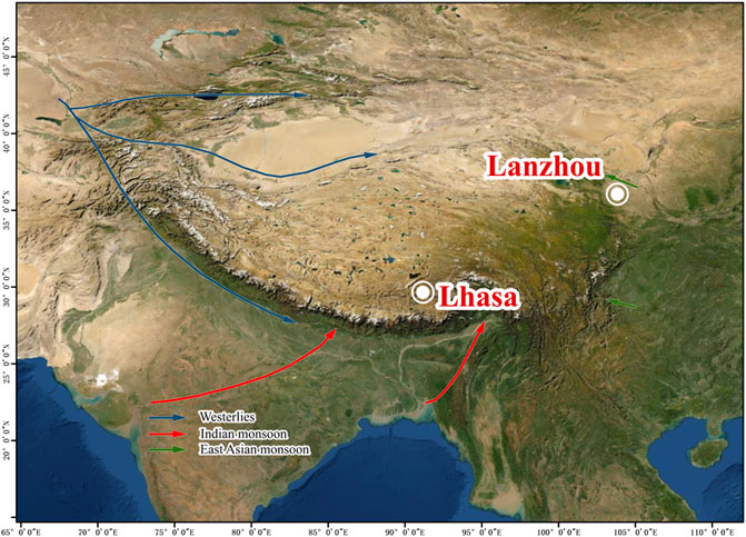
FIGURE 1. Location of the cities of Lanzhou and Lhasa.
By investigating the climate–REC relationships in Lanzhou and Lhasa and determining the projected impacts of climate change, the results of this study provide new insights for future climate–energy studies of the cold season and can be used to inform policies for regional climate adaptation. The algorithm model developed herein is also readily compatible with potential early-warning projects to protect against extreme weather-induced power outages.
2 Materials and Methods
2.1 Research Design
Previous studies have suggested that factors impacting REC include temperature, precipitation, income, population, and urbanization (Auffhammer and Aroonruengsawat, 2011; Deschênes and Greenstone, 2011; Auffhammer and Mansur, 2014; Davis and Gertler, 2015; Frederiks et al., 2015; Fan et al., 2017; Li et al., 2019). Since urbanization in essence is the process of rural population moving to urban areas, and Lanzhou and Lhasa are both urban areas, the factor of urbanization can be reflected by population in these two cities. Thus, the model was constructed using temperature, precipitation, income, and population as predictor variables, and REC was used as the response variable. Unlike previous studies that used data modeling, an algorithm modeling approach was adopted. With respect to the predictive accuracy and interpretability, the results from the model developed herein were compared with those of the parameter-based models used previously to verify and demonstrate the strength of this new modeling approach. The capacities of the new model to holistically estimate and project climatic impacts were used to determine the projected impacts of climate change on REC under the RCP 2.6, 4.5, and 8.5 scenarios.
2.2 Data
The estimates of this study was based on panel data for the period of 2011–2019 in Lanzhou and for the period of 2014–2019 in Lhasa. According to the data source (to be specified later), before 2014, REC data for Lhasa was compromised by wholesale consumption that cannot be differentiated from residential use. Therefore, we only used after-2014 REC data for Lhasa, which resulted in the inconsistent study periods of the two cities. As this study investigates the impacts of climate change, changes in both the mean temperature and precipitation, as well as their seasonal variations were included. Each dataset included monthly REC, monthly mean temperature, monthly precipitation, annual salary, and annual population. The study periods were mainly defined by the availability of monthly REC data for the two cities. Obtaining more than 5 years of monthly REC observations from Lhasa is difficult, as the grid company has changed how REC is calculated several times over recent decades. Since the constructed panel dataset must include the REC, this study had to settle for a shorter study period to construct the model. The model results are reliable as long as the model validation is sound (i.e., does not exhibit overfitting).
Lanzhou REC data was obtained from the Gansu State Grid Company (GSGC), while Lhasa REC data was obtained from the Tibet State Grid Company (TSGC). Monthly mean temperatures and monthly precipitation data were calculated using daily temperature and precipitation data for 2011–2019 in Lanzhou and for 2014–2019 in Lhasa, which were obtained from the China Meteorological Administration (https://data.cma.cn/en). Annual salary and population data were obtained from the National Bureau of Statistics of China (https://data.stats.gov.cn/english/).
To predict future climatic impacts on REC in Lanzhou and Lhasa, we used future climate projections for China, which are based on the regcm4.6 model under the RCP 2.6, 4.5, and 8.5 scenarios (Lei and Xiaoduo, 2020). This regional climate model has yielded more accurate simulation results of the present mean climatology over Northwest China than those of the Met Office Hadley Centre Earth System (HadGEM2-ES) global climate model (Pan et al., 2020). Climate projections were extracted for Lanzhou and Lhasa from the nearest available locations in the data (i.e., at 36° N, 103.5° E for Lanzhou and at 29.5° N, 91° E for Lhasa). This climate projection data is more reliable for Lanzhou, as it is located in Northwest China where the regcm4.6 model performs well. However, Lhasa is located not only in Southwest China, but also on the Tibetan Plateau. While the Tibetan Plateau is increasingly becoming warmer and wetter (Yao et al., 2019), climate projections for the region are complicated substantially by the uplift of the Tibetan Plateau, and reliable near-term climate change projections are not yet available (Hu and Zhou, 2021). Since Lanzhou is also projected to become warmer and have increased precipitation (Lei and Xiaoduo, 2020), we were able to obtain a qualitative perspective for Lhasa from the results obtained for Lanzhou.
2.3 Methods
2.3.1 Algorithm Vs Data Models
Algorithm modeling was used in this study rather than data modeling, which has been used by previous studies. Modeling is a process that associates predictor variables with the response variable. The main difference between data modeling and algorithm modeling is the way in which the association is constructed (Breiman, 2001). Data modeling assumes that real-world data conform to a stochastic regression function that incorporates predictor variables, random noise, and parameters. The model then attempts to estimate the response variable using functions that are validated using goodness-of-fit tests (Breiman, 2001). In contrast, algorithm modeling assumes that the association is unknown and attempts to identify an algorithm that can best predict the response variable using the predictor variables. The results are then validated using the predictive accuracy (Breiman, 2001). Algorithm and data modeling are known as randomized and distributional approaches, respectively, in the computer science community. The two modeling types are considered to be two sides of the same coin, as algorithm modeling approximates the best performance with probabilities, while data modeling uses parameters to obtain the best performance (Yao, 1977)
Data models attempt to fit real-world observational data for various systems with unknown mechanisms into a parametric model selected by a statistician. This inevitably compromises the accuracy, as well as the insight of the model (Breiman, 2001). Despite efforts to minimize parametric assumptions (Deschênes and Greenstone, 2011), the econometric models used in previous studies remain parameter-based data models with similar limitations. Conversely, algorithm modeling is entirely data-driven, as it makes only one assumption, i.e., that the data were obtained from an unknown multivariate distribution (Breiman, 2001). A model with a higher accuracy yields more reliable information regarding the underlying data mechanism. Since algorithmic models have generally been shown to make better predictions (Breiman, 2001), we adopted algorithm modeling in this study.
Since algorithm modeling treats the association between the predictor and response variables as unknown, there was no means of ensuring that the algorithm worked well with the data prior to testing. We derived a pool of seven commonly used candidate algorithms (Brownlee, 2016), three of which were basic algorithms: k-nearest neighbors (KNN), support vector regression (SVR), and classification and regression tree (CART). The KNN algorithm is designed with the assumption that similar things are in close proximity to each other. It makes estimations by measuring the distances between an instance and all other instances in the dataset, then selects the specified number of instances (K) closest to the point of interest, then votes for the most frequent label (in the case of classification) or averages the labels (in the case of regression) (Altman, 1992). SVR works by constructing a hyperplane or hyperplanes in a high-dimensional space for either classification or regression. The hyperplane with the longest distance from all of the nearest training data points of any class (also known as the functional margin) is considered to be a good separation, as a larger margin yields a lower generalization error (Cortes and Vapnik, 1995). CART is also known as a decision tree, since it is a tree-like algorithm that is constructed by repeatedly splitting into two child nodes. It splits on a single input variable that improves the Gini index, which is a performance measure that calculates the probability of a specific input variable being classified incorrectly when selected randomly (Breiman et al., 2017). The structure of CART makes it (along with other tree-based algorithms) innately immune to correlations among the predictor variables (Friedman et al., 2001).
The other four algorithms were ensemble algorithms, which is a machine learning method that combines several base algorithms to decrease the variance and bias or to improve predictions. We used Adaptive Boosting (AB), Random Forest (RF), Extra Trees (ET), and Gradient Boosting Machine (GBM), all of which are CART ensembles with different ensemble methods. The RF and ET algorithms train their individual trees independently and average the predictions across trees, which is an ensemble method known as bagging. RF and ET differ in how their individual trees split, as well as how they sample the data. RF splits where the performance measurement is best, whereas ET splits randomly. RF sub-samples the data sample with replacement or bootstrapping, while ET uses the original data sample (Ho, 1995; Geurts et al., 2006). The AB and GBM algorithms build one tree at a time, wherein each new tree corrects errors made by the previous tree, which is an ensemble method known as boosting. AB and GBM differ in how they identify and correct errors of previous trees. AB identifies errors using high-weight data points as each new tree up-weights the observations that were misclassified by the previous tree, whereas GBM identifies errors using the gradient of loss function computed in the previous tree, which reflects how well the previous tree performed. AB corrects errors by assigning its trees different weights in the final prediction based on their performance. In contrast, GBM weights all trees equally, but restricts their predictive capacities through the learning rate, which represents how quickly an error is corrected from each tree to the next, for greater accuracy (Mason et al., 1999; Friedman, 2001; Kégl, 2013).
The baseline performance of the seven algorithms was determined by running the data with each algorithm using the default hyperparameters of the algorithms in a Python 3.7 environment with scikit-learn implementation (Pedregosa et al., 2011). The scikit-learn utility of Pipeline (Pedregosa et al., 2011) was used to automate the workflow and avoid data leakage. In the workflow, we standardized the data to test all candidate algorithms. In the study, 80% of the data was used for algorithm testing and modeling and 20% reserved for validation. The training data and the reserved validation data were split randomly. And 10-fold cross validation was used to estimate the algorithmic performance as measured by the mean squared error (MSE).
The stochastic nature of machine learning algorithms means that the model results for each run can differ. To ensure that we selected the best algorithm from the candidate pool, each of the seven candidate algorithms was run 100 times on the data and their performances were averaged in terms of the MSE and averaged ranking out of 100 runs.
For comparison, a simple multivariate parameter-based ordinary least squares (OLS) model is also used in parallel with the algorithm model as follows:
where
2.3.2 Comparing Predictive Accuracies
Figure 2 shows the baseline performances of the candidate algorithms using the Lanzhou and Lhasa data, respectively. The GBM ensemble algorithm was the best fit for the Lanzhou data during 2011–2019 data and the Lhasa data during 2014–2019, as it exhibited the lowest average MSEs with a high consistency.
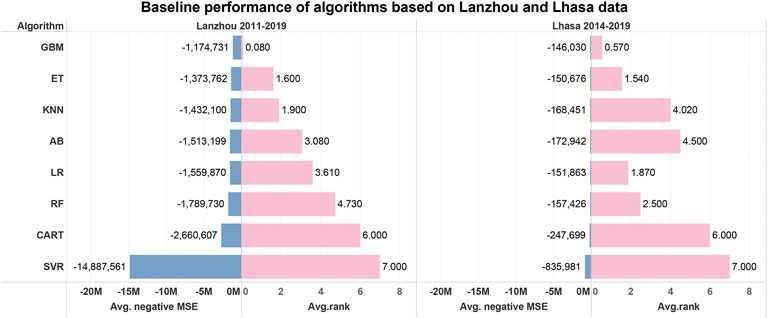
FIGURE 2. Results of algorithm selection for estimating Lanzhou and Lhasa residential electricity consumption (REC). Blue bars indicate negative mean squared error (MSE) and pink bars indicate the average ranking for each algorithm based on 100 runs. Shorter bars indicate a better baseline performance of the corresponding algorithm (GBM - gradient boosting machine, ET - extra trees, KNN - k-nearest neighbors, AB- adaptive boosting, RF - random forest, CART - classification and regression tree, SVR - support vector regression, LR - simple linear regression model, i.e., the ordinary least squares (OLS) model).
To validate the model results in case of overfitting, the predictor variables from the validation datasets were run with the prepared models to make predictions. The validation results are shown in Figure 3. The low MSE results suggest that the model was not overfitted. This indicates the strength of the algorithm model to make predictions based on limited data points.
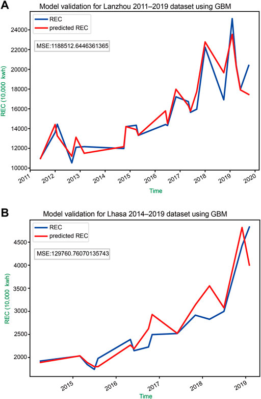
FIGURE 3. Validation of the Lanzhou and Lhasa models. The blue line marks the reserved residential electricity consumption (REC) validation data. The red line indicates REC estimated using the corresponding model with temperature, precipitation, income, and population inputs. (A) and (B) show the validation results for models trained using datasets for Lanzhou during 2011–2019 and for Lhasa during 2014–2019, respectively.
2.3.3 Comparing the Interpretability of the Models
A robust interpretation of the models can only be achieved with models that exhibit high predicative accuracies. Figures 2, 3 indicate that the GBM yielded the highest predicative accuracy for both the Lanzhou and Lhasa data. To compare its interpretation with those of the traditional parameter-based models, Table 1 presents the results of the OLS linear models across different datasets. Table 1 indicates that the OLS models can explain 90.1% of the variation in the Lanzhou year-round data and 85.1% of the variation in the Lhasa data during 2014–2019. Hence, it was meaningful to compare the OLS interpretation with the GBM model interpretation for Lanzhou, as both were good models for the Lanzhou data, with the GBM yielding better predictions (Figure 2).
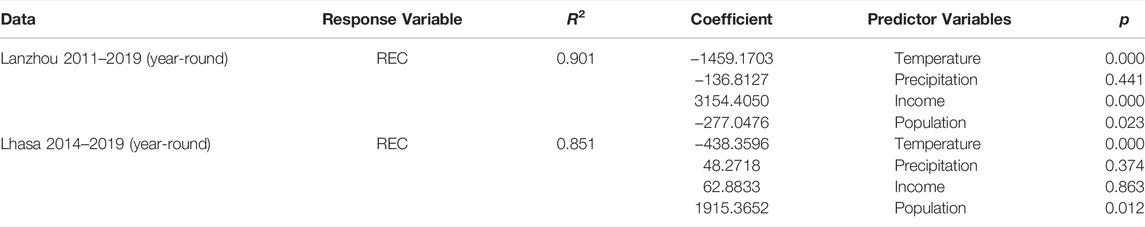
TABLE 1. Results of ordinary least squares (OLS) linear regression modeling of the Lanzhou and Lhasa year-round datasets. (REC - residential electricity consumption).
Despite their reputation for being “black boxes” that are difficult to interpret (Azodi et al., 2020), algorithmic models have been shown to be interpretable in ways that not only show the individual impacts of the predictor variables, but also the joint impact of multiple predictor variables (Friedman, 2001; Friedman and Meulman, 2003; Strobl et al., 2007; Goldstein et al., 2015; Zhao and Hastie, 2019; Azodi et al., 2020; Mehdiyev and Fettke, 2020; Molnar, 2020). We used partial dependence (PDP) and individual conditional expectation (ICE) plots to interpret the data mechanisms underlying the algorithmic models (Zhao and Hastie, 2019; Mehdiyev and Fettke, 2020; Molnar, 2020). We used the concept of feature to discussion the PDPs and ICE plots. The concepts of “feature” and “predictor variable” are often used interchangeably, particularly in machine learning models. However, we made a distinction between the two in this study for clarity. We use the term “predictor variables” to refer to individual variables we used for the modeling (i.e., temperature, precipitation, income, and population). A “feature” can either be an individual predictor variable, such as temperature, or two combined predictor variables (e.g., climate, which comprises both temperature and precipitation).
The PDPs depict the overall dependence of model prediction on a given input feature by marginalizing over the values of all other input features. ICE plots disaggregate this average by showing the estimated functional relationship of each instance (Goldstein et al., 2015; Zhao and Hastie, 2019; Mehdiyev and Fettke, 2020; Molnar, 2020). While PDPs are useful for depicting the overall marginal effect of a given feature, they can also obscure heterogeneous relationships caused by interactions (Friedman and Meulman, 2003; Goldstein et al., 2015; Zhao and Hastie, 2019; Mehdiyev and Fettke, 2020; Molnar, 2020). For this reason, we compared the ICE plots and PDPs to determine whether heterogeneous relationships were present in the estimations.
The PDP utility offered by scikit-learn (Pedregosa et al., 2011) was adopted for the ICE and PDP visualizations. To compare with the OLS interpretation based on coefficients for the predictor variables, the study first interpreted the roles of the predictor variables for the GBM model, as shown in Figure 4. Note that the marginal effect is not the predicted REC value; rather, it is the way in which the REC changes with the feature. All of the ICE plot curves generally followed the same pattern indicated by the PDP line. This means that the PDPs of the models provided a reliable interpretation of the relationships between the features and REC.
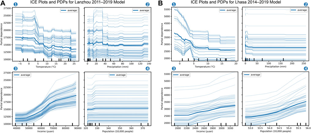
FIGURE 4. Individual conditional expectation (ICE) plots and partial dependence plots (PDPs) for the models. Results of model estimates for REC in (A) Lanzhou during 2011–2019 and for (B) Lhasa during 2014–2019. Subplots ①, ②, ③, and ④ show the partial dependences of temperature, precipitation, income, and population, respectively.
Interpretations using the GBM and OLS models on individual predictor variables were generally consistent for the temperature‒REC relationships, with the innately non-linear GBM being more informative than the OLS model. The GBM suggests that precipitation plays a role in influencing REC, whereas the OLS appeared to differ since it failed to reach a conclusion on the role of precipitation, as shown by the high p-value and the opposite signs of the precipitation coefficients for the two cities (Table 1). At this stage, we cannot be sure which interpretation is correct, owing to the multi-collinearity between the year-round temperature and precipitation data, as shown in Figures 5A,C.
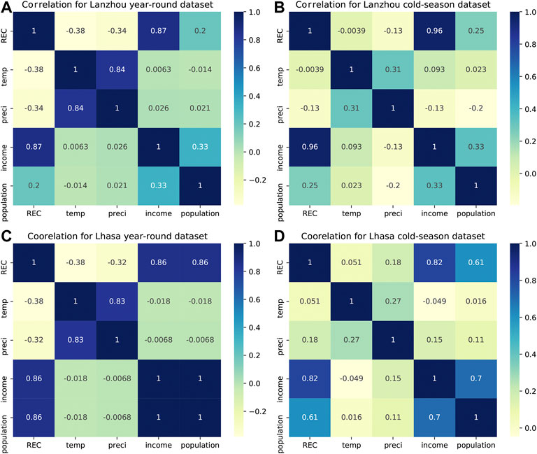
FIGURE 5. Correlation heat maps of the 2011–2019 Lanzhou and 2014–2019 Lhasa data. Correlations among the data variables in the Lanzhou (A) year-round and (B) cold season datasets and correlations for the Lhasa (C) year-round and (D) cold season datasets. (REC - residential electricity consumption).
Multi-collinearity may be one of the reasons why precipitation has not been fully considered in previous studies. Multi-collinearity can reduce the precision of the estimated coefficients in linear regressions and it is common to remove or lessen the weight of one predictor (in this case, precipitation). Correlations between temperature and precipitation are also challenging for the GBM interpretation, as the use of PDPs and ICE plots is based on the assumption that the features are not correlated (Zhao and Hastie, 2019; Mehdiyev and Fettke, 2020; Molnar, 2020).
tTo test our hypothesis regarding the role of precipitation during the cold season, the study created a data subset comprising data from November, December, January, and February, i.e., the cold season only. Multi-collinearity between temperature and precipitation in this subset was no longer a problem for either city, as shown in Figures 5B,C. For this reason, this study used this subset (rather than the year-round dataset) to analyze the individual roles of temperature and precipitation.
Quantification of year-round climatic impacts should be conducted without interference from multi-collinearity. Interpretations of an algorithm model can manage the multi-collinearity between temperature and precipitation by combining them into one feature (Molnar, 2020). Unlike OLS models that can only rely on individual predictor variable coefficients for information, the PDPs of algorithmic models can be applied to a predictor variable, as well as to a feature comprising two combined predictor variables (Friedman and Meulman, 2003; Goldstein et al., 2015; Molnar, 2020). Since the climate feature was not correlated with the other features of the model in this study, our interpretations of the climatic impacts were not affected by the influence of multi-collinearity.
It is noteworthy that the PDP for the climate feature was not a simple combination of the individual PDPs for temperature and precipitation, as shown in Figure 4. Rather, the PDP for the climate feature captured changes in temperature and precipitation, as well as their interactions, and showed the marginal effects of these components as a whole, since partial dependence was calculated by marginalizing over all the other inputs of the estimation (i.e., income and population) (Friedman and Meulman 2003; Molnar 2020). When quantifying the marginal effect of the climate feature, a newly developed method was used: First, the monthly mean temperature and monthly precipitation were averaged by calendar month to represent the corresponding mean climatic patterns for Lanzhou and Lhasa during their respective study periods; then the potential variation ranges for the climate patterns using the standard deviations of the monthly mean temperature and monthly precipitation were obtained for each calendar month in both cities; finally, the average marginal effects of climate for each calendar month in each of the two cities were obtained by averaging the marginal effects of all the climate conditions within the variation range for each month (Xia et al., 2022).
Built on the method mentioned above, this study further tapped into the potential of the algorithm model for holistically quantifying the climatic impacts on REC to predict the impacts of climate change on REC in Lanzhou and Lhasa. This was achieved by replacing the climate observations with RCP 2.6, RCP 4.5, and RCP 8.5 climate projections in the PDP-based quantification. The climate projections were summarized into monthly mean climate as follows:
Where
Then the marginal effects of all climate instances within the variation range of
Where
Where
3 Results
3.1 Individual Temperature and Precipitation Roles
The GBM and OLS interpretations described in Section 2.3.3 indicate a negative effect of temperature on REC in both cities, which is consistent with the heating “half” of the U-shaped temperature–REC function obtained in previous studies (Auffhammer and Mansur, 2014; Li et al., 2019). Combined with local knowledge, we are confident that the climatic impacts on the REC in Lanzhou and Lhasa are mainly driven by heating consumption. However, fewer evidences were available from previous studies regarding the role of precipitation, and neither the OLS coefficient nor the GBM PDPs were conclusive in this respect. To test our hypothesis regarding the role of precipitation during the cold season, we ran the OLS model using the cold season data subset and obtained the results presented in Table 2.
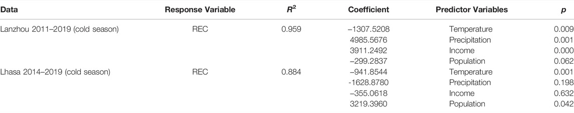
TABLE 2. Results of ordinary least squares (OLS) linear regression modeling of the Lanzhou and Lhasa cold-season data subsets. (REC - residential electricity consumption).
The OLS model based on the Lanzhou cold-season data subset yielded an R2 of 95.9% and considers precipitation to be a statistically significant predictor variable, with a p-value lower than that of temperature. The positive precipitation coefficient suggests that more precipitation during the cold season will drive up REC. The cold season data subset was too small to model using GBM; however, we were able to obtain confirmation based on its year-round interpretation. In Figure 4, the GBM indicates that the marginal effects of precipitation on REC are higher when monthly precipitation falls below 40 mm in Lanzhou and below 20 mm in Lhasa. Climate patterns in the two cities (Figures 6B,D) indicate that such low monthly precipitation only occurs during the cold season, suggesting that the impact of precipitation is stronger during the cold season.
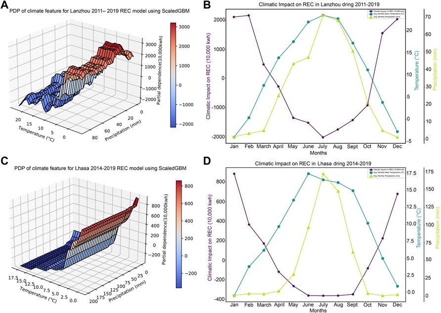
FIGURE 6. Partial dependence plot (PDP)-based interpretation of gradient boosting machine (GBM) models for the 2011–2019 Lanzhou and the 2014–2019 Lhasa year-round datasets. Marginal effects of all climate conditions considered by the GBM model on residential electricity consumption (REC) in (A) Lanzhou and (C) Lhasa, with x-axes showing temperature, y-axes showing precipitation, and z-axes showing the marginal effect of the climate feature on the model outcome. Average climatic impacts based on climate patterns in (B) Lanzhou and (D) Lhasa, with x-axes showing the month, purple y-axes showing the marginal effect of the climate feature or climatic impact, blue y-axes showing temperature, and green y-axes showing precipitation.
The OLS model for the Lhasa cold season data subset yielded an R2 of 88.4% and suggests a negative precipitation–REC relationship. No statistically significant precipitation–REC relationship was obtained in this case, although the p-value for precipitation was considerably lower for the Lhasa cold season data subset than for the year-round Lhasa data. Despite this, the result can be used as a parallel evidence, as the statistical community has warned that it would be inappropriate to conclude that there is no association simply because the p-value is >0.05, i.e. statistical significance (Amrhein et al., 2019). We compared the p-values with results of GBM models to verify the role of precipitation during cold season. The GBM interpretation of the precipitation impact in Lhasa (Figure 4B) also confirmed this theory, as it exhibited a small peak for a low precipitation range during the cold season, suggesting the existence of a precipitation impact during the cold season.
An explanation of the absence of a positive OLS coefficient for precipitation during the cold season in Lhasa was identified by comparing the climate patterns of Lhasa and Lanzhou, as shown in Figure 6B,D. The monthly mean temperature rarely drops much below 0 °C in Lhasa, even during the cold season. In addition, monthly precipitation during the cold season in Lhasa is considerably lower than that during the cold season in Lanzhou. In other words, compared with Lanzhou, snowfall is not as frequent or as heavy in Lhasa; thus, the impact of precipitation during the cold season in Lhasa is less observable. This study concluded that the impact of precipitation was stronger in both cities during the cold season as a result of snowfall, which increased electricity consumption used for heating.
3.2 Climatic Impacts
As discussed in Section 2.3.3, quantifying the marginal effects of year-round temperature and precipitation separately would not be accurate due to the presence of multi-collinearity. It is unreasonable to omit either temperature or precipitation from our estimation just because of their numerical correlation, as we have already shown that both play roles as independent climate variables that influence REC. For this reason, we quantified their joint impact (i.e., the climatic impact) by interpreting the climate feature enabled by the PDP. Figures 6A,C show the marginal effects of climate on REC and the climatic impacts on REC in Lanzhou and Lhasa, respectively. We used real-world climate patterns in Figures 6B,C to assist in constraining the way in which we used the PDPs such that the conclusions were not obtained based on extremely unlikely temperature and precipitation combinations. A climatic impact of zero indicates that the climate feature did not have any effect on the estimation. Positive climatic impact values indicate that the corresponding climatic conditions will increased the estimated REC, while negative values indicate reductions in REC. We hereafter describe changes in the climatic impacts by referring to them as positive or negative climatic impacts; i.e., when we state that the climatic impact was enhanced, this means that the climatic impact has increased its absolute value.
Interpretation of the GBM model using a holistic climate feature (Figure 6B) exhibits a V-shaped relationship between the climatic impact on REC and calendar month for Lanzhou, with July exhibiting the strongest negative climatic impact and November, December, January, and February exhibiting the largest positive climatic impacts. The change in the climatic impact during the cold season was more consistent with the change in precipitation, which agrees with our previous finding that precipitation has a stronger impact on REC in Lanzhou during the cold season, likely in the form of snowfall given that the mean temperatures during the cold season months were slightly above or below 0 C.
In Lhasa, the relationship between the climatic impact on REC and calendar month was U-shaped (Figure 6D), with June, July, August, and September exhibiting similarly strong negative climatic impacts, and December and January exhibiting the largest positive climatic impacts. The change in climatic impact during the cold season was more consistent with the change in temperature than the change in precipitation. This can be explained by the fact that less snowfall occurs in Lhasa. Precipitation is low in Lhasa during the cold season, during which only 1 month has a mean temperature below 0 C.
Although ‘V-’ and ‘U-shaped’ were used to describe the PDP curves, the curves were completely different from the U-shaped curves commonly discussed in previous studies. This study moved beyond the temperature-based climate–REC concept to include temperature, precipitation, and seasonal variations in the climate–REC relationship. While the U-shaped curves discussed in previous studies reflect the temperature-–REC relationship, the V- and U-shaped curves in this study reflect the monthly/seasonal variations in climatic impacts, including the effects of both temperature and precipitation on REC. The lower end of the V- and U-shaped curves exhibited negative REC responses to climate during the warm season, and positive REC responses during the cold season, suggesting that climate impacts REC in different directions during the warm and cold seasons. In other words, REC in Lanzhou and Lhasa is mostly driven by the heating demand, as a strong cooling demand would be reflected as a positive response during the warm season. This is consistent with local knowledge that residents of both cities do not commonly use air conditioners for cooling during the warm season. In this case, for a city with both strong heating and cooling demands, we would expect a W-shaped PDP curve. The V- and U-shaped curves obtained for Lanzhou and Lhasa, respectively, indicate that REC in Lanzhou is more sensitive to climatic variations during the warm months than REC in Lhasa.
It is also notable that the temperature threshold for climatic impacts on REC in the two cities was not consistent, as opposed to the assumptions of HDD and CDD that there is a consistent base temperature at which there is no energy demand for cooling or heating. Climatic impacts on REC are approximately zero when the monthly mean temperature is ∼12 °C in Lanzhou and ∼8 °C in Lhasa. This further supports our point that temperature alone does not determine the climatic impact on REC. It is inferred that precipitation, as well as socioeconomic factors, also play a role in determining the climate threshold when there is no energy demand for cooling or heating.
3.3 Projected Changes in Climatic Impacts on REC
To obtain meaningful comparisons of climatic impacts on REC under status-quo and the projected RCP 2.6, 4.5, and 8.5 scenarios, insights are needed regarding the biases of the simulated climate patterns. A smaller simulated bias indicates a more reliable projected climatic impact. We compared the climate patterns simulated by the Regcm4.6 model under the different climate scenarios for Lanzhou and Lhasa with the observed climate patterns during 2011‒2019 and 2014–2019, respectively. The data used to train the model developed herein was considered as the status-quo condition. Figures 7A,B show comparisons of the status-quo and simulated temperature patterns, and Figures 7C,D show the precipitation patterns.
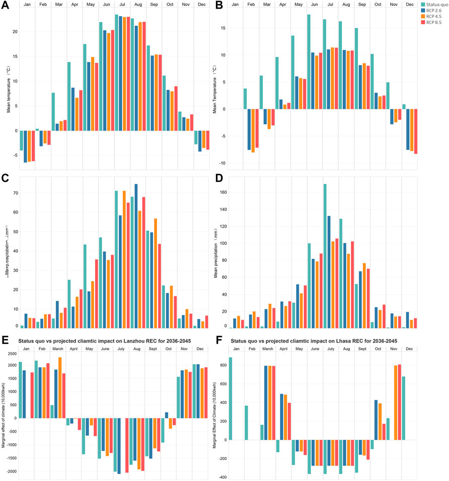
FIGURE 7. Projected climate change and change in climatic impact on residential electricity consumption (REC) in Lanzhou and Lhasa. Comparisons of observed and simulated monthly mean temperatures for status-quo periods in (A) Lanzhou and (B) Lhasa. Comparison of observed and simulated monthly mean precipitation for status-quo periods in (C) Lanzhou and (D) Lhasa. Comparisons between the status-quo climatic impacts on REC with those under the projected climate scenarios during 2036‒2045 in (E) Lanzhou and (F) Lhasa. Status-quo data are marked in green, RCP 2.6 data in blue, RCP 4.5 data in orange, and RCP 8.5 data in red.
For Lanzhou, the simulated temperatures were lower than observed temperatures under all three climate scenarios, although they were within an accepted range (with the exception of February and March). The simulated temperature in February was <0 °C across all scenarios, while the actual observed temperature was >0 °C. This may create confusion, given that our hypothesis is dependent on precipitation taking the form of snowfall. The underestimation of the simulated temperature during March was too large to be used. For Lhasa, the simulated temperatures were considerably lower than the observed temperatures under all three climate scenarios throughout the year, with the cold season months all exhibiting negative simulated values, while the observed temperatures were positive.
For precipitation, the Regcm4.6 model overestimated precipitation during the cold season months in both Lanzhou and Lhasa under all scenarios, with Lanzhou exhibiting a much smaller (and thus more acceptable) bias throughout the year than Lhasa. Thus, the climatic impact projection for Lanzhou is more reliable than that for Lhasa. With this consideration, the climatic impacts on REC under the status-quo scenario with those under the RCP 2.6, 4.5, and 8.5 climate scenarios for Lanzhou and Lhasa were compared (Figures 7E,F). The absence of projections under some scenarios was the result of projected climate conditions exceeding the boundaries of the PDPs defined by the status-quo observational data.
For Lanzhou, February and March were excluded from this discussion due to the unacceptable bias during these months. During the cold season, climatic impacts on REC were projected to increase in November, and decreased only slightly in December and January for the period of 2036‒2045. The climatic impact in November would increase more under RCP 2.6 and 4.5 than under RCP 8.5, and would decrease less in December under RCP 2.6 than under RCP 4.5 or 8.5. The positive climatic impacts on REC were projected to increase or decrease less during the cold season for scenarios exhibiting slower warming rates (i.e., RCP 2.6), suggesting an offsetting role of precipitation. In other words, although warming reduces REC during the cold season, increased precipitation increases REC during the cold season in Lanzhou. This result indicates that precipitation has an offsetting effect to temperature on cold season REC in Lanzhou.
For the remainder of the year, only July, August, and September exhibited enhanced negative climatic impacts. This also suggests an offsetting role of precipitation, as warming alone would only enhance the negative climatic impacts. Since July and August (i.e., the two warmest months in Lanzhou) will still experience negative climatic impacts, we do not believe that the decrease in negative impact during the other months is driven by cooling-related demands. Rather, a more logical explanation is that more precipitation may have a cooling effect, which will offset the warming impact on REC. This offsetting impact of precipitation may be sufficiently strong to change the climatic impact. For example, the climatic impact under RCP 2.6 during October changed from negative to positive, suggesting that the climatic impact changed from reducing the REC estimation to increasing it. This can be confirmed by the fact that negative climatic impacts were generally more enhanced under RCP 8.5 than under RCP 2.6. The varying rankings of the climatic impacts under RCP 4.5 for the three scenarios suggest that, under this scenario, the effects of precipitation and temperature have competing importances for shaping the overall climatic impact.
The quantifications of climatic impacts on REC in Lhasa was not thoroughly interpreted, as the simulated climate was considered to be excessively biased, thereby making interpretations of the projected climatic impacts on REC extremely difficult. However, as Lhasa, like Lanzhou, is becoming warmer and wetter over time, we also inferred that the impact of precipitation will likely offset the warming impact on REC. However, as Lanzhou exhibited a stronger precipitation impact during the cold season and was more sensitive to climate during warm months, we expect that Lanzhou will be affected by this offsetting effect more than Lhasa.
4 Conclusion
The results indicate that the climatic impacts on REC in both Lanzhou and Lhasa are driven by heating-related demand. The model results support the hypothesis regarding the role of precipitation. Both Lanzhou and Lhasa exhibited stronger precipitation impacts during the cold season, this confirms previous evidence that precipitation (particularly snowfall) boosts electricity consumption during the cold season. The impact was stronger in Lanzhou, which has more months when the temperature is below 0 °C experiences and more precipitation during the cold season. As the two cities become warmer and wetter, precipitation will offset the impact of warming on REC throughout the year, with Lanzhou being more affected. Based on the projections for Lanzhou, the offsetting effect was more pronounced during the cold season across all scenarios, and was particularly strong under RCP 2.6. For the remainder of the year, the effects of increased precipitation and warming will have competing importances under the RCP 4.5 scenario, while the effects of temperature will generally dominate the climatic impacts under the RCP 8.5 scenario.
5 Discussion
This study shows the strength of algorithm modeling, as it exhibits improved predictive accuracy and interpretability for studying climatic impacts on REC than linear models. Compared with previous econometric models used in climate–REC studies, the method described herein allows highly correlated temperature and precipitation data to be interpreted as one climate feature to quantify the climatic impact. This allowed us to treat temperature and precipitation equally, which has the potential for use in all climatic impact studies.
A data-driven model can only be as good as the data. The model developed herein failed to make predictions for several scenarios that exceeded the bounds of the PDPs of the climate feature. This study was also limited, as we controlled the non-climate inputs at the status-quo level to predict the climatic impacts on REC; however, socioeconomic conditions will definitely alter REC and the marginal effects of the climatic impacts. Future studies should have a socioeconomic focus to enable more accurate predictions. The projection obtained for Lhasa was also limited by insufficient climate projection studies in the region. More accurate climate projections are needed to improve the understanding of potential future climatic impacts on REC in southern China.
This study highlights the need for climate-related energy studies to holistically address climate, rather than to focus solely on temperature, particularly in regions with cold winters, as well as in areas vulnerable to extreme weather such as blizzards. The findings provide previously unavailable insights for future cold season climate–energy studies, particularly for regions with cold baseline climate but are getting more precipitation such as the Tibetan Plateau and its surroundings. As this study shows that precipitation and temperature impact REC in opposite ways in cold season in the region, strong increase in precipitation during the cold season may offset the REC reduction supposedly brought by warming. This study can thus be used to assist with regional policy-making regarding climate change adaptations. The PDP-based projection developed herein is also readily compatible with potential early-warning projects, as it can be easily replicated with high frequency panel data and can make predictions based on weather forecasts, which will help to protect against power outages induced by extreme weather.
Data Availability Statement
The data that supports the findings of this study are available from data sources as stated in Section 2.2. Restrictions apply to the availability of the REC data, which were used under license for this study. Data are available from the authors with the permission of data sources.
Author Contributions
TY designed the research, analyzed the data and secured the research funding. CX designed and performed the research, analyzed the data, and wrote the paper. HH reviewed the model. PW analyzed the data.
Funding
This work was supported by the Second Tibetan Plateau Scientific Expedition and Research (STEP) project (Grant No. 2019QZKK0208) and the Strategic Priority Research Program of the Chinese Academy of Sciences (Grant No. XDA20100300).
Acknowledgments
The authors are grateful for the helpful comments received on an earlier preprint version (Xia et al., 2021), as well as the coordination efforts led by Dr. Weicai Wang from the STEP project office and the Third Pole Environment (TPE) program office.
Conflict of Interest
The authors declare that the research was conducted in the absence of any commercial or financial relationships that could be construed as a potential conflict of interest.
Publisher’s Note
All claims expressed in this article are solely those of the authors and do not necessarily represent those of their affiliated organizations, or those of the publisher, the editors and the reviewers. Any product that may be evaluated in this article, or claim that may be made by its manufacturer, is not guaranteed or endorsed by the publisher.
References
Aljazeera (2022). Huge US Winter Storm Leaves More Than 330,000 without Power, Online. Available at: https://www.aljazeera.com/news/2022/2/4/huge-us-winter-storm-leaves-more-than-330000-without-power (Accessed March 1, 2022).
Altman, N. S. (1992). An Introduction to Kernel and Nearest-Neighbor Nonparametric Regression. Am. Statistician 46, 175–185. doi:10.1080/00031305.1992.10475879
Amrhein, V., Greenland, S., and Mcshane, B. (2019). Scientists Rise up against Statistical Significance. Nature. 567, 305–307. doi:10.1038/d41586-019-00857-9
Auffhammer, M., and Aroonruengsawat, A. (2011). Simulating the Impacts of Climate Change, Prices and Population on California's Residential Electricity Consumption. Clim. change 109, 191–210. doi:10.1007/s10584-011-0299-y
Auffhammer, M., Baylis, P., and Hausman, C. H. (2017). Climate Change Is Projected to Have Severe Impacts on the Frequency and Intensity of Peak Electricity Demand across the United States. Proc. Natl. Acad. Sci. U.S.A. 114, 1886–1891. doi:10.1073/pnas.1613193114
Auffhammer, M., and Mansur, E. T. (2014). Measuring Climatic Impacts on Energy Consumption: A Review of the Empirical Literature. Energy Econ. 46, 522–530. doi:10.1016/j.eneco.2014.04.017
Azodi, C. B., Tang, J., and Shiu, S.-H. (2020). Opening the Black Box: Interpretable Machine Learning for Geneticists. Trends Genet. 36, 442–455. doi:10.1016/j.tig.2020.03.005
Breiman, L., Friedman, J., Olshen, R., and Stone, C. (2017). Classification Regression Trees. Routledge. Milton Park, Abingdon-on-Thames, Oxfordshire, England, UK.
Breiman, L. (2001). Statistical Modeling: The Two Cultures (With Comments and a Rejoinder by the Author). Stat. Sci. 16, 199–231. doi:10.1214/ss/1009213726
Busby, J. W., Baker, K., Bazilian, M. D., Gilbert, A. Q., Grubert, E., Rai, V., et al. (2021). Cascading Risks: Understanding the 2021 Winter Blackout in Texas. Energy Res. Soc. Sci. 77, 102106. doi:10.1016/j.erss.2021.102106
Cohen, J., Screen, J. A., Furtado, J. C., Barlow, M., Whittleston, D., Coumou, D., et al. (2014). Recent Arctic Amplification and Extreme Mid-latitude Weather. Nat. Geosci. 7, 627–637. doi:10.1038/ngeo2234
Cortes, C., and Vapnik, V. (1995). Support-vector Networks. Mach. Learn 20, 273–297. doi:10.1007/bf00994018
Davis, L. W., and Gertler, P. J. (2015). Contribution of Air Conditioning Adoption to Future Energy Use under Global Warming. Proc. Natl. Acad. Sci. U.S.A. 112, 5962–5967. doi:10.1073/pnas.1423558112
Deschênes, O., and Greenstone, M. (2011). Climate Change, Mortality, and Adaptation: Evidence from Annual Fluctuations in Weather in the US. Am. Econ. J. Appl. Econ. 3, 152–185. doi:10.3386/w13178
Du, K., Yu, Y., and Wei, C. (2020). Climatic Impact on China's Residential Electricity Consumption: Does the Income Level Matter? China Econ. Rev. 63, 101520. doi:10.1016/j.chieco.2020.101520
Fan, J.-L., Zhang, Y.-J., and Wang, B. (2017). The Impact of Urbanization on Residential Energy Consumption in China: An Aggregated and Disaggregated Analysis. Renew. Sustain. Energy Rev. 75, 220–233. doi:10.1016/j.rser.2016.10.066
Frederiks, E., Stenner, K., and Hobman, E. (2015). The Socio-Demographic and Psychological Predictors of Residential Energy Consumption: A Comprehensive Review. Energies 8, 573–609. doi:10.3390/en8010573
Friedman, J., Hastie, T., and Tibshirani, R. (2001). The Elements of Statistical Learning. New York: Springer Series in Statistics.
Friedman, J. H. (2001). Greedy Function Approximation: a Gradient Boosting Machine. Ann. Statistics, 29, 1189–1232. doi:10.1214/aos/1013203451
Friedman, J. H., and Meulman, J. J. (2003). Multiple Additive Regression Trees with Application in Epidemiology. Stat. Med. 22, 1365–1381. doi:10.1002/sim.1501
Geurts, P., Ernst, D., and Wehenkel, L. (2006). Extremely Randomized Trees. Mach. Learn 63, 3–42. doi:10.1007/s10994-006-6226-1
Goldstein, A., Kapelner, A., Bleich, J., and Pitkin, E. (2015). Peeking inside the Black Box: Visualizing Statistical Learning with Plots of Individual Conditional Expectation. J. Comput. Graph. Statistics 24, 44–65. doi:10.1080/10618600.2014.907095
Ho, T. K. (1995). “Random Decision Forests,” in Proceedings of 3rd international conference on document analysis and recognition: IEEE, Montreal, QC, Canada, 14-16 Aug. 1995, 278–282.
Hu, S., and Zhou, T. (2021). Skillful Prediction of Summer Rainfall in the Tibetan Plateau on Multiyear Time Scales. Sci. Adv. 7, eabf9395. doi:10.1126/sciadv.abf9395
Kégl, B. (2013). The Return of AdaBoost. Mh. Multi-class Hamming trees. arXiv [Preprint]. Available at: https://arxiv.org/abs/1312.6086#.
Lei, Z., and Xiaoduo, P. (2020). “Future Climate Projection of China Based on regcm4.6 (2007-2099),” in National Tibetan Plateau Data Center. Editor C. National Tibetan Plateau Data.
Li, Y., Pizer, W. A., and Wu, L. (2019). Climate Change and Residential Electricity Consumption in the Yangtze River Delta, China. Proc. Natl. Acad. Sci. U.S.A. 116, 472–477. doi:10.1073/pnas.1804667115
Mason, L., Baxter, J., Bartlett, P., and Frean, M. (1999). “Boosting Algorithms as Gradient Descent in Function Space,” in Proceedings of the NIPS, Denver, CO, United States, November 29–December 4, 1999, 512–518.
Mehdiyev, N., and Fettke, P. (2020). Prescriptive Process Analytics with Deep Learning and Explainable Artificial Intelligence.
Mideksa, T. K., and Kallbekken, S. (2010). The Impact of Climate Change on the Electricity Market: A Review. Energy policy 38, 3579–3585. doi:10.1016/j.enpol.2010.02.035
Molnar, C. (2020). Interpretable Machine Learning. Lulu press. Morrisville, North Carolina, United States
Nordhaus, W. D. (2017). Revisiting the Social Cost of Carbon. Proc. Natl. Acad. Sci. U.S.A. 114, 1518–1523. doi:10.1073/pnas.1609244114
Pan, X., Zhang, L., and Huang, C. (2020). Future Climate Projection in Northwest China with RegCM4. 6. Earth Space Sci. Rev. 7, e2019EA000819. doi:10.1029/2019ea000819
Pedregosa, F., Varoquaux, G., Gramfort, A., Michel, V., Thirion, B., Grisel, O., et al. (2011). Scikit-learn: Machine Learning in Python. J. Mach. Learn. Res. 12, 2825–2830.
Strobl, C., Boulesteix, A. L., Zeileis, A., and Hothorn, T. (2007). Bias in Random Forest Variable Importance Measures: Illustrations, Sources and a Solution. BMC Bioinforma. 8, 25–21. doi:10.1186/1471-2105-8-25
Waite, M., Cohen, E., Torbey, H., Piccirilli, M., Tian, Y., and Modi, V. (2017). Global Trends in Urban Electricity Demands for Cooling and Heating. Energy 127, 786–802. doi:10.1016/j.energy.2017.03.095
Xia, C., Yao, T., Hou, H., and Wang, P. (2021). Impact of Climate Change on Residential Electricity in Western Cities in China.
Xia, C., Yao, T., Wang, W., and Hu, W. (2022). Effect of Climate on Residential Electricity Consumption: A Data-Driven Approach. Energies 15, 3355. doi:10.3390/en15093355
Yao, A. C.-C. (1977). “Probabilistic Computations: Toward a Unified Measure of Complexity,” in 18th Annual Symposium on Foundations of Computer Science (sfcs 1977): IEEE Computer Society), Providence, RI, USA, 31 October 1977 - 02 November 1977, 222–227.
Yao, T., Masson-Delmotte, V., Gao, J., Yu, W. S., Yang, X. X., Risi, C., et al. (2013). A Review of Climatic Controls on Delta O-18 in Precipitation over the Tibetan Plateau: Observation and Simulations. Rev. Geophys. 51, 20023. doi:10.1002/rog.20023
Yao, T., Xue, Y., Chen, D., Chen, F., Thompson, L., Cui, P., et al. (2019). Recent Third Pole's Rapid Warming Accompanies Cryospheric Melt and Water Cycle Intensification and Interactions between Monsoon and Environment: Multidisciplinary Approach with Observations, Modeling, and Analysis. Bull. Am. Meteorological Soc. 100, 423–444. doi:10.1175/bams-d-17-0057.1
Zhang, M., Zhang, K., Hu, W., Zhu, B., Wang, P., and Wei, Y.-M. (2020). Exploring the Climatic Impacts on Residential Electricity Consumption in Jiangsu, China. Energy Policy 140, 111398. doi:10.1016/j.enpol.2020.111398
Zhao, Q., and Hastie, T. (2019). Causal Interpretations of Black-Box Models. J. Bus. Econ. Statistics 39, 272–281. doi:10.1080/07350015.2019.1624293
Zheng, X. (2020). Power Utilities Asked to Ensure Proper Supply, Online. Available at:. https://global.chinadaily.com.cn/a/202012/19/WS5fdd5583a31024ad0ba9cc79.html (Accessed.
Keywords: climate impact, cold-season, precipitation, residential electricity consumption, machine learning, heating
Citation: Xia C, Yao T, Hou H and Wang P (2022) Mixed Impact of Climate Change on Cold Season Residential Electricity: A Case Study of Lanzhou and Lhasa. Front. Earth Sci. 10:908259. doi: 10.3389/feart.2022.908259
Received: 30 March 2022; Accepted: 22 June 2022;
Published: 22 July 2022.
Edited by:
Xander Wang, University of Prince Edward Island, CanadaCopyright © 2022 Xia, Yao, Hou and Wang. This is an open-access article distributed under the terms of the Creative Commons Attribution License (CC BY). The use, distribution or reproduction in other forums is permitted, provided the original author(s) and the copyright owner(s) are credited and that the original publication in this journal is cited, in accordance with accepted academic practice. No use, distribution or reproduction is permitted which does not comply with these terms.
*Correspondence: Cuihui Xia, eGlhY3VpaHVpQGl0cGNhcy5hYy5jbg==