 Li Q. Ming1
 Zhao Z. Yun
- 1Institute of Science and Technology, NCUT, Beijing, China
- 2School of Energy and Mining, CUMTB, Beijing, China
- 3China Academy of Safety Science and Technology, Beijing, China
- 4School of Safety Engineering, CUMTB, Beijing, China
Because of the continuous exploitation of metal minerals and the limited availability of land resources, many tailings ponds have been expanded. It is of great importance to dynamically calculate the critical parameters of flooding and sand velocity after a collapse, and quickly determine the dangerous area downstream on reducing the hidden dangers for an accident. In view of the limitations of the single finite element and discrete element methods for the simulation of tailings pond instability, the authors use the finite element and discrete element coupling method (GDEM) for the first time to carry out a dynamical process for numerical simulation of the evolution of a tailings pond collapse. The sediment movement and submerged range were compared with the results of the Volume of Fluid (VOF) method. The comparison shows that the change in drainage flow at the dam foundation position and the depth change in the downstream sensitive point after the dam break are consistent with the VOF calculation results, which indicates that the GDEM can be used as an effective means for the analysis of tailings dam failure. The calculation results of this method can provide technical support for the determination of dangerous areas downstream of tailings ponds and the safety management of key areas.
1 Introduction
The majority of China’s metal deposit resources are deeply buried low-grade ores, while high-grade ores are relatively scarce. As a result, a large number of tailings ponds are required to store mining byproducts. A total of 7,793 tailings ponds were present in the country by the end of 2017, with the highest tailings dam reaching 325 m (Yin et al., 2018). Because of the continuous exploitation of metal minerals and the limited availability of land resources, many tailings ponds have been expanded. The gradually increasing heights and slopes of tailings ponds have induced multiple failures of tailings dams throughout the country, leading to high loss of life, mineral resources, and state property (Li et al., 2015; Zhang et al., 2016). Thus, it is important to establish an effective numerical model that can simulate the unique flow of tailings pond slurry. Such a model would provide the means to quickly simulate tailings dam failure and immediately analyze the severity of failure incidents, and quantitatively divide at-risk areas downstream, thereby improving the safety management of downstream areas and reducing the severity of failure-induced damage.
The methods of numerically simulating tailings ponds can be divided into two types: The finite element methods and the discrete element methods. The finite element methods are based on continuum mechanics and are mainly used to simulate the continuous deformation and plastic failure of materials (Brzezinski, 2002; Zandarín et al., 2009). The failure analysis was carried out by establishing finite element model, and the damage of materials was evaluated numerically (Guo et al., 2020; Arafa et al., 2022; Tang et al., 2022). They can be further divided into the finite element method (Peter and Mahmood, 2003; Wang et al., 2011) and the finite difference method (Chakrabotry and Choudhury, 2009) and used to study the stability of tailings dam slopes and tailings ponds. The discrete element methods are based on discontinuous medium mechanics and are used to simulate the motion and collision characteristics of a bulk system. They can be further divided into two types, namely, block discrete element modelling and particle discrete element modelling. Presently, discrete element methods focus on the relationship between macro-and micromechanics (Fakhimi et al., 2002; Backstrom et al., 2008; Hsieh et al., 2008; Feng et al., 2014; Wang et al., 2014) and rock slope stability (Esaki et al., 1998; Xu et al., 2022), whereas limited research has been conducted on the stability of tailings ponds. The tailings pond discharge fluid is a mixture of tailings sand and water. The single finite element method does not easily realize the simulation of the movement process of microscopic particles in the process of tailings pond destruction. Although the single discrete element method can exhibit the dynamic process of damage, it does not easily reflect the whole process from the start of the dam failure to the end.
The continuum-based discrete element method (GDEM) software combines the continuum-based discrete element method (CDEM) and high-performance graphics processing unit (GPU) technology (Li et al., 2004; Zou et al., 2007; Zhang et al., 2019). CDEM couples the finite element method (FEM) with the discrete element method (DEM) to conduct finite element calculations inside block elements and discrete element calculations at block boundaries, which facilitates simulating the entire process from continuous deformation to fracture movement (Feng et al., 2014). The GDEM can be widely applied to progressive failure simulations and overall stability evaluations of materials in several engineering fields, including geotechnical, mining, tunnel, oil and gas, water conservancy, geological, and structural engineering.
To accurately analyze the tailings sediment movement, the inundation range, and the impact on sensitive targets downstream during the failure process of tailings dams, the present study applies GDEM numerical simulation for the first time to test the failure evolution of a tailings dam. The whole process of dam break of tailings pond was analyzed, thereby achieving a dynamic simulation of the entire failure process. In addition, the impact of tailings dam failure on sensitive targets downstream is determined by analyzing the movement of tailings slurry during the failure process, thereby providing theoretical and technical support for the safety management of tailings ponds, especially for downstream reservoir areas.
CDEM is a discrete element method based on continuum mechanics. By combining the finite element and discrete element methods, CDEM not only facilitates simulations of the continuous or discontinuous deformation and the movement of granular material under static and dynamic loading but also models the progressive failure of materials, from continuum to discontinuum (Nezami et al., 2004; Yeung et al., 2007).
The governing equation of the CDEM is the equation of particle motion (Li et al., 2007). In Eq. 1,
where
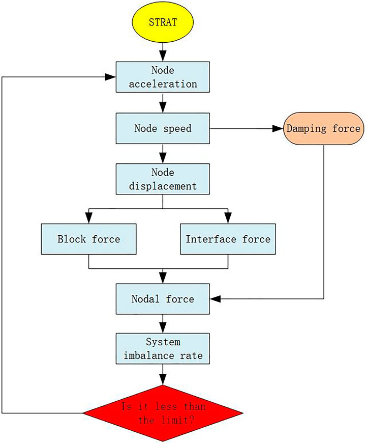
FIGURE 1. CDEM calculation process.
In CDEM, a discrete block can consist of one or more FEM elements (as shown in Figure 2). A continuum-based constitutive model and finite element approach are used inside the blocks, whereas a discontinuum-based constitutive model and discrete element approach are used for the block interfaces (Li et al., 2007; Feng et al., 2014). The CDEM finite elements can be simple tetrahedrons, pentahedrons, and hexahedrons, or complex polyhedrons (Figure 3). The discontinuous deformation is modeled by springs placed between the CDEM blocks, such that spring breakage simulates the cracking and slipping of material.
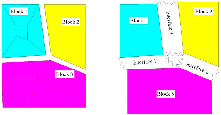
FIGURE 2. Blocks and interfaces in CDEM.
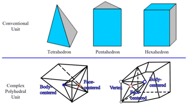
FIGURE 3. Finite element unit in CDEM.
The CDEM uses the element stiffness matrix to obtain the deformation force generated by blocks. That is, the nodal force of the elements is obtained using the already known element stiffness matrix and the nodal displacement. Because the CDEM uses the dynamic relaxation method, the entire stiffness matrix need not be formed; rather, only obtaining the element stiffness matrix of each element is sufficient. At each iteration, the nodal force of the element itself is calculated using Eq. 2 and assigned to the corresponding node element. Among them,
The normal and tangential springs of the CDEM contact surfaces are shown in Figure 4, where
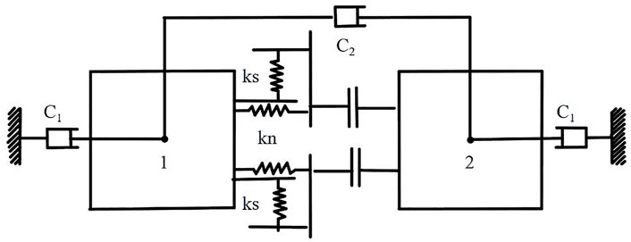
FIGURE 4. Schematic of the contact surface normal and tangential springs.
The spring force can be calculated using Eq. 3, in which
When calculating element failure, the spring force is modified using the Mohr-Coulomb criterion and tensile criterion, as shown in Eq. 4.
where, T is tensile strength,
2 Materials and Methods
2.1 Principles of GDEM Method
The core of GDEM is continuous-discontinuous element method (CDEM) based on Lagrange equation, which organically combines finite element and discrete element. Block is used to characterize the continuum properties of materials, and interface is used to characterize the discontinuum properties of materials. The gradual failure process of materials is simulated through the fracture of block boundary and interior.
GDEM is used to simulate dam break, which can intuitively show the impact range of tailings dam break and effectively analyze the failure of tailings dam.
2.2 A Real Case of a Tailing Pond
2.2.1 Descriptions on Geological Settings
The case tailings pond is surrounded by mountains on three sides. It is multiditched to form a claw-shaped valley. The surface of the mountain is a Quaternary slope, and some of the rocks are bare. The coverage by mountain vegetation is high, and the growth is general. There are Yingyun dioritic gneisses in the Shachang Formation of the Mishan Group in the Archean Period. Some parts of the red feldspar are more distinctive than others and have felsic veins.
The overall terrain of the site is relatively high and has little precipitation, the rock mass has no obvious water-collecting structure. The seismic fortification intensity is 7 degrees, and the basic acceleration of the designed earthquake is 0.15 g.
2.2.2 Working Conditions
The tailings pond has two initial dams, both of which are permeable rockfill dams. The elevation of the west dam is 149.3 m, and the elevation of the east dam is 143.5 m. The top width of the two dams is 5 m, the ratio of the inner and outer slopes is 1:2.0, and the elevation of the dam is 207 m. The final stacking height of the designed tailings is 220 m, comprising approximately 13.5 million m3, and the dam has a service life of 20 years.
The tailings accumulation dam is above the 163.5 m elevation of the dam crest at the beginning of the tailings pond. The dam slope has a total of 4 terraces at elevations of 173.5, 183.5, 193.5, and 203.5 m, and the mound width is 5 m, with a slope ratio of 1:4.5, as shown in Figure 5.
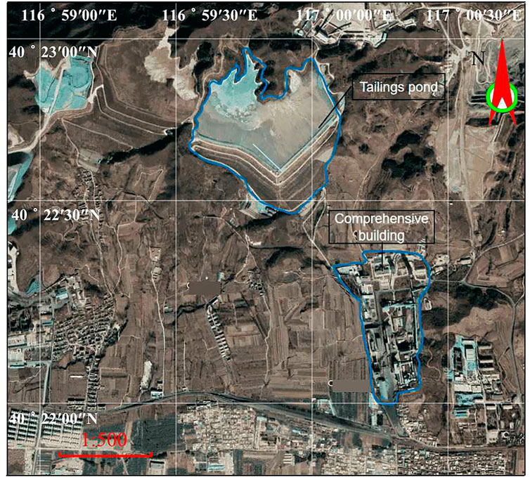
FIGURE 5. Satellite image of tailings pond simulation area.
Within 800 m downstream of the tailings pond, it is mainly farmland. There are railways and highways passing through approximately 1,000 m south of the tailings pond. There are three villages, machine repair workshops, mineral processing workshops, and comprehensive buildings downstream, with a total of 2,000 people.
2.3 Failure Analysis of the Tailing Pond Dam
2.3.1 Numerical Model Conditions
The tailings flow after dam failure is a free surface flow problem with a moving boundary and complex large deformation. The tailings flow after the failure is simulated using the smoothed particle hydrodynamics (SPH) method, which eliminates problems associated with entanglement and distortion; these are common to the traditional Eulerian grid method. As a result, the SPH method is uniquely advantageous in dealing with large-deformation free-surface and moving-boundary problems. It is highly suitable for simulating the tailings slurry flow after dam failure. To ensure the accuracy of the calculation results, the following assumptions were made about the model:
1) The tailings pond consists of countless discrete microparticles;
2) The tailings pond is made of a homogeneous material, and each part of the pond has the same physical properties;
3) The spatial model of the tailings pond is filled with continuous nonporous particles.
Assumed dam failure mode: the length of the breach is 350 m from the east-west dam junction, and the dam break depth to the bottom of the dam is 149.3 m at the bottom of the west dam and 143.5 m at the bottom of the east dam; the tailings pond water level is 207 m.
Assumed failure discharge: the total sediment discharge is taken as the total volume of water and tailings in the reservoir above 207 m; a total of 6 million cubic meters of tailings and water are discharged.
Flow resistance at the bottom of the total flow discharge: the change in the Manning coefficient is a function of the shear force; it simulates the flow characteristics of the tailings slurry, which are different from those of water; the relationship between the shear force and the Manning coefficient in the model is shown in Figure 6.
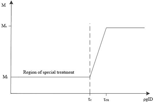
FIGURE 6. Relationship between shear force and the Manning coefficient.
Where, τc is the critical shear force at which the tailings slurry begins to flow; τcu is the critical shear force at which the tailings slurry changes from a yield-pseudoplastic fluid to a Bingham plastic fluid; Ml is the minimum Manning coefficient, which characterizes the bottom friction when the tailings slurry begins to flow; Mu is the maximum Manning coefficient, which characterizes the bottom friction when the tailings slurry changes from a yield-pseudoplastic fluid to a Bingham plastic fluid.
2.3.2 Modelling Procedure
During the analysis of the tailings dam failure, the area affected by the tailings pond is divided using unstructured triangular elements. The unstructured triangular mesh has the advantages of high adaptability for complex areas, flexible local encryption, and convenient self-adaptation. This method can effectively simulate natural boundaries and complex underwater topography and improves the accuracy of boundary simulations.
Figure 7 shows the topographic map of the area and the designed stacked tailings dam generated in the CAD model.
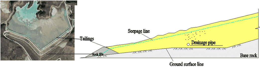
FIGURE 7. Topographic map of the Earth’s surface and tailings dam.
The terrain surface and the dam model files are imported into the GDEM software. Next, the key surface points are stripped to form a NURBS surface. Finally, the surface model of the tailings dam is formed using the geometry-create-volume-by-contour command.
The terrain surface and the dam model are meshed. The terrain surface is divided into a 2D planar mesh, whereas the dam model is divided into a 3D particle mesh, ultimately generating 105,585 triangular terrain surface elements and 119,427 dam model particles.
The JavaScript script file is written from four aspects: as shown in Figure 8, setting the mechanical properties and material parameters of the particle model, calculating the critical parameters of the dam, and monitoring the data point, the solution step number, and the resulting output interval. The mechanical properties and material parameters of the case tailings library are shown in Table 1. The mechanical parameters of tailings were obtained by carrying out geotechnical tests on tailings, and were used as experimental parameters of this model.
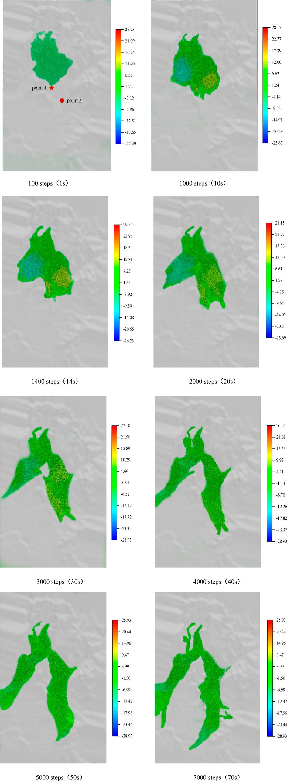
FIGURE 8. Simulation results of tailings dam failure range at different times.
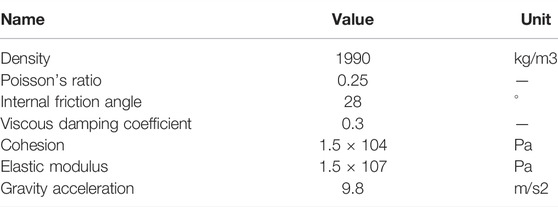
TABLE 1. List of simulated particulate material parameters.
3 Results
3.1 Analysis of the Dam Failure Results
In Figure 8, Point one refers to the monitoring point at the foot of the dam, and Point two refers to the monitoring point of the comprehensive building. In the initial stage of the tailings pond failure, the mud gradually spreads from the dam site and then gradually diffuses into the low-lying area. Due to the high middle of the terrain and the low east and west sides, two mudflows gradually form downstream. After 1 min, the mud basically covers the entire calculation area. As the mud continues to flow to the lower area and out of the calculation area, the mud depth in the calculation area continuously decreases, and the submerged range shrinks, as shown in the flooding map at 70 s.
The failure process of a stacked dam can be divided into three stages: the initial stage of accelerated collapse, the intermediate stage of decelerated diffusion, and the final stage of stable accumulation. Steps 0 to 600 (0–6 s) are the initial stage of the accelerated collapse after the failure. During this stage, the tailings flow out of the tailings pond and diffuse rapidly westward, forming a fan-shaped collapse zone. Steps 600 to 5,500 (1–55 s) form the intermediate stage of the decelerated diffusion. During this stage, the tailings particles continue to pour out of the tailings pond; however, the particle velocity decreases gradually as their travel distance increases. At 5,500 steps, the velocity of the particles in the front of the flow tends to zero; however, the middle part of the tailings flow continues to move forward slowly. Steps 5,500 to 9,500 (55–95 s) are the final stage of stable accumulation. During this stage, most of the tailings particles are discharged from the tailings pond, and the tailings flow distribution does not change significantly. At this point, all the particles have zero velocity, and the dam failure process ends.
The calculation results of the submerged depth and flow rate of the case tailings pond reaching the downstream complex after the dam break are shown in Table 2. The flow velocity and quantity changes during the dam break process are shown in Figures 9, 10. The flow velocity and submerged depth during the tailings impact of the comprehensive building are shown in Figures 11, 12.
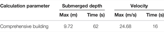
TABLE 2. Results of the downstream sensitive target for the #1 tailings dam failure simulation.
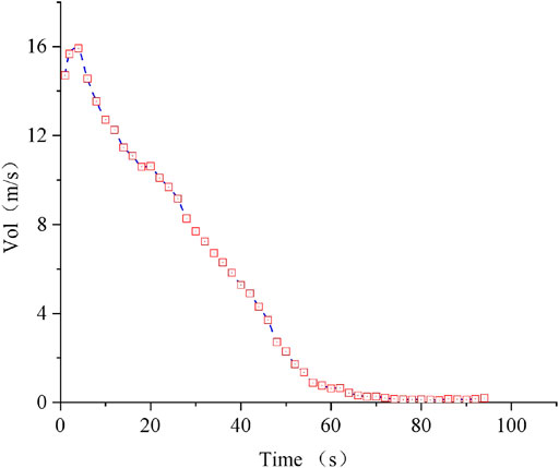
FIGURE 9. Change in sediment velocity at the bottom of the tailings dam.
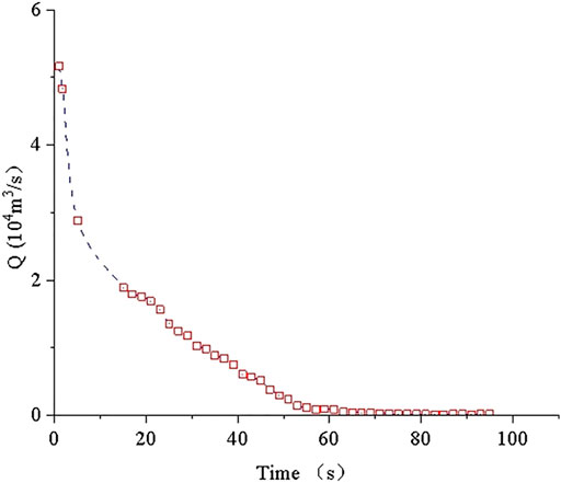
FIGURE 10. Change in quantity of flow at the bottom of the tailings dam.
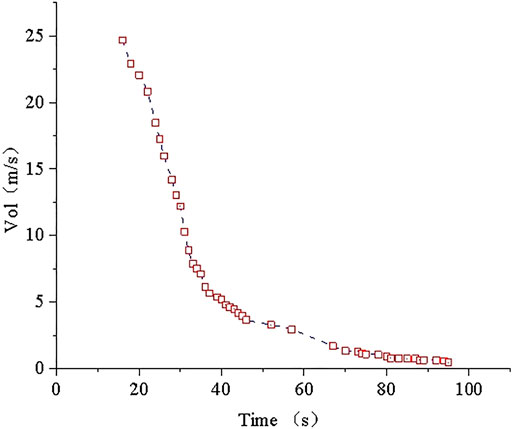
FIGURE 11. Change in sediment flow rate at the comprehensive building.
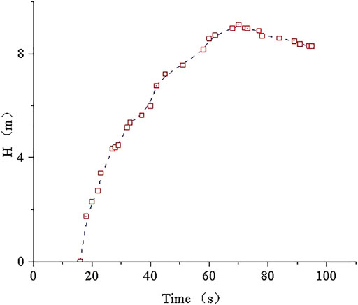
FIGURE 12. The overflow depth of the comprehensive building.
In Figures 9–12, the tailings instantaneous impact velocity after the dam breaks is 14.71 m/s with the maximum quantity of flow 51643 m3/s, and the maximum flow rate reaches 16.47 m/s in the 3rd second. As the volume of tailings in the reservoir continuously decrease, the velocity of the tailings flowing through the dam bottom gradually decrease. Finally, the tailings reach a steady-state in the 55th second, and the discharge flow rate is 0.97 m/s, which gradually approaches zero.
The tailings reach the downstream comprehensive building in the 16th second after the dam break, and the instantaneous flow rate is 24.68 m/s. Due to terrain effects, the impact tailing speed gradually decreases. After 80th second, the flow rate is gradually stabilized and finally reaches a steady state. The maximum overflow depth of the complex is 9.72 m, and the corresponding time is the 62 s after the occurrence of the collapse.
3.2 Comparative Analysis of the Calculation Results of Volume of Fluid
The Volume of Fluid (VOF) model tracks the volume of each fluid by solving a set of momentum equations and continuous equations that simulate the motion of two or more fluids that are not blended.
As shown in Figures 13, 14. The VOF adopts all the model breaks instantaneously to calculate and obtain the process line of the fracture flow. When the water level is 207 m and the upstream flow is not considered, the storage capacity is 6 million m3, and the time required is 150 s. The peak flow of the fracture is 270,000 m3/s, the maximum mud depth at the downstream comprehensive building is 1.45 m, and the corresponding time is 30 s after the occurrence of the collapse.
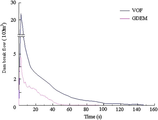
FIGURE 13. The comparison of tailings dam break flow between VOF and GDEM.
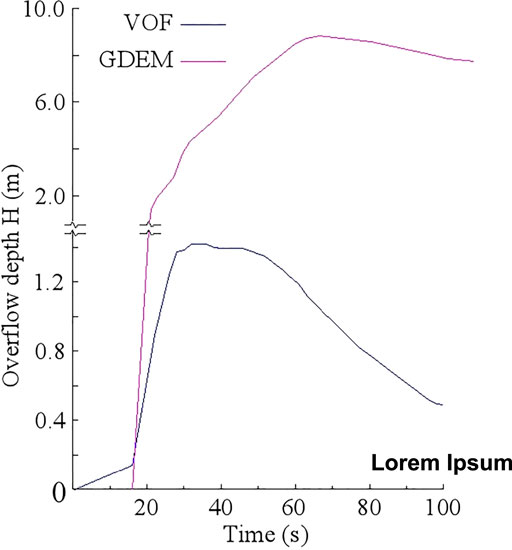
FIGURE 14. The comparison of comprehensive buildings overflow depth.
The comparison between the calculation results of the GDEM and the VOF method shows that the trend of the flow curve at the bottom is consistent, and there is a certain difference between the flow values. The change in the depth of the sediment that reaches the complex after the collapse is consistent, but the mud depth values are different.
By analyzing the calculation principle of the two methods, the two monitoring methods are shown to be different. The monitoring part of the GDEM adopts the arrangement monitoring ring method to monitor the discharge flow at the bottom of the dam body and in a certain area at the comprehensive building. The VOF calculates the discharge flow generated by the instantaneous discharge of all the broken sediments. The VOF method calculation of the discharge flow at the bottom of the tailings dam is higher than that of the GDEM. The VOF calculation does not consider the downstream topographic changes, and the downstream ground is set to the plane flow. The GDEM introduces the tailings pond and surrounding terrain into the original scale, which can truly reflect the change in the sediment flow after the tailings pond breaks, so the time of sediment flow in the VOF method is shorter than that in the GDEM. Comparison of the results of the two methods shows that the GDEM can effectively reflect the change in sediment flow after the tailings pond collapse and proves that the method can be used as an effective analysis method for tailings pond failure analysis.
4 Conclusion and Discussion
1) The process of tailings dam failure can be divided into three stages: accelerated collapse, decelerated diffusion and stable accumulation. During the initial stage of accelerated collapse, the tailings flow diffuses rapidly westward, forming a fan-shaped collapse zone. During the intermediate stage of diffusion, the tailings particles continue to pour out from the tailings pond; however, the particle velocity gradually decreases and eventually stabilizes. During the final stage of stable accumulation, most of the tailings particles are discharged from the tailings pond, the tailings discharge flow is basically stable, and the distribution of the tailings flow does not have any significant changes; thus, the dam failure process ends.
2) The time of the dam-sludge mud-sand flow reaching the comprehensive building is 16 s, and the instantaneous impact velocity is 24.68 m3/s. The maximum submerged depth is 9.72 m at the 62 s. The final dam-sludge sand flow at the 83rd second tends to be stable at the comprehensive building. The experimental results show that once the tailings dam fails, it will have a serious impact downstream, seriously threatening the lives and property of the downstream residents. It is necessary to strengthen the safety management of the tailings pond to prevent the occurrence of dam failure.
3) Comparing the dam break calculation with the VOF method, the change in the discharge flow at the dam foundation position and the submerged depth at the downstream sensitive point after the dam break is consistent, which proves that the GDEM can be used for effective measurement in the tailings dam failure analysis.
4) A new large scale model is used to calculate the whole process of tailings dam failure. Using the GDEM to simulate dam failure can visually determine the impact range after tailings failure and then determine the dam break safety boundary. This method provides a quantitative approach for judging the stability of the tailings pond; in addition, it can effectively simulate the dam-break process and can be used as one of the methods to measure the stability of tailings pond failure. It also proves the feasibility of the GDEM in the evaluation of the stability of tailings ponds.
Data Availability Statement
The original contributions presented in the study are included in the article/supplementary material, further inquiries can be directed to the corresponding author.
Author Contributions
All authors listed have made a substantial, direct, and intellectual contribution to the work and approved it for publication.
Funding
This work is supported by the National Natural Science Fund of China (Grant Number. 51874260).
Conflict of Interest
The authors declare that the research was conducted in the absence of any commercial or financial relationships that could be construed as a potential conflict of interest.
Publisher’s Note
All claims expressed in this article are solely those of the authors and do not necessarily represent those of their affiliated organizations, or those of the publisher, the editors and the reviewers. Any product that may be evaluated in this article, or claim that may be made by its manufacturer, is not guaranteed or endorsed by the publisher.
References
Arafa, I. T., Elhosseiny, O. M., and Nawar, M. T. (2022). Damage Assessment of Perforated Steel Beams Subjected to Blast Loading. Structures 40, 646–658. doi:10.1016/j.istruc.2022.04.051
Bäckström, A., Antikainen, J., Backers, T., Feng, X., Jing, L., Kobayashi, A., et al. (2008). Numerical Modelling of Uniaxial Compressive Failure of Granite with and without Saline Porewater. Int. J. Rock. Mech. Min. 45, 1126–1142. doi:10.1016/j.ijrmms.2007.12.001
Brzezinski, L. S. (2002). Static Liquefaction as a Possible Explanation for the Merriespruit Tailings Dam Failure: Discussion. Can. Geotech. J. 39, 1439–1440. doi:10.1139/t02-078
Chakrabotry, D., and Choudhury, D. (2009). Investigation of the Behavior of Tailings Earthen Dam under Seismic Conditions. Amc. J. Eng. App. Sci. 2, 559–564. doi:10.3844/ajeassp.2009.559.564
Esaki, T., Jiang, Y., hattarai, T. N., Nozaki, A., and Mizokami, T. (1998). Stability Analysis and Reinforcement System Design in a Progressively Failed Steep Rock Slope by the Distinct Element Method. Int. J. Rock. Mech. Min. 35, 664–666.
Fakhimi, A., Carvalho, F., Ishida, T., and Labuz, J. F. (2002). Simulation of Failure Around a Circular Opening in Rock. Int. J. Rock. Mech. Min. 39, 507–515. doi:10.1016/s1365-1609(02)00041-2
Feng, C., Li, S., Liu, X., and Zhang, Y. (2014). A Semi-Spring and Semi-Edge Combined Contact Model in CDEM and its Application to Analysis of Jiweishan Landslide. J. Rock. Mech. Geotech. Eng. 6, 26–35. doi:10.1016/j.jrmge.2013.12.001
Feng, Y. T., and Owen, D. R. J. (2014). Discrete Element Modelling of Large Scale Particle Systems-I: Exact Scaling Laws. Comput. Part. Mech. 1, 159–168. doi:10.1007/s40571-014-0010-y
Guo, Z., Chen, L., Yin, K., Shrestha, D. P., and Zhang, L. (2020). Quantitative Risk Assessment of Slow-Moving Landslides from the Viewpoint of Decision-Making: A Case Study of the Three Gorges Reservoir in China. Eng. Geol. 273, 105667. doi:10.1016/j.enggeo.2020.105667
Hsieh, Y.-M., Li, H.-H., Huang, T.-H., and Jeng, F.-S. (2008). Interpretations on How the Macroscopic Mechanical Behavior of Sandstone Affected by Microscopic Properties-Revealed by Bonded-Particle Model. Eng. Geo. 99, 1–10. doi:10.1016/j.enggeo.2008.01.017
Li, Q.-M., Yuan, H.-N., and Zhong, M.-H. (2015). Safety Assessment of Waste Rock Dump Built on Existing Tailings Ponds. J. Cent. South Univ. 22, 2707–2718. doi:10.1007/s11771-015-2801-6
Li, S. H., Wang, J. G., Liu, B. S., and Dong, D. P. (2007). Analysis of Critical Excavation Depth for a Jointed Rock Slope by Face to Face Discrete Element Method, Rock. Mech. Rock. Eng. 40, 331–348. doi:10.1007/s00603-006-0084-9
Li, S., Zhao, M., Wang, Y., and Rao, Y. (2004). A New Numerical Method for DEM-Black and Particle Model. Int. J. Rock. Mech. Min. 41, 414–418. doi:10.1016/j.ijrmms.2004.03.076
Nezami, E. G., Hashash, Y. M. A., Zhao, D., and Ghaboussi, J. (2004). A Fast Contact Detection Algorithm for 3-D Discrete Element Method. Comput. Geotech. 31, 575–587. doi:10.1016/j.compgeo.2004.08.002
Peter, M. B., and Mahmood, S. K. (2003). “Seismic Stability of Impoundments,” in Proceedings of the 17th VGS on Geotechnical Engineering for Geoenvironmental Application, Vancouver, British Columbia, January, 77–84.
Tang, Y., Guo, Z., Wu, L., Hong, B., Feng, W., Su, X., et al. (2022). Assessing Debris Flow Risk at a Catchment Scale for an Economic Decision Based on the LiDAR DEM and Numerical Simulation. Front. Earth Sci. 10, 821735. doi:10.3389/feart.2022.821735
Wang, T., Zhou, Y., Lv, Q., Zhu, Y., and Jiang, C. (2011). A Safety Assessment of the New Xiangyun Phosphogypsum Tailings Pond. Miner. Eng. 24, 1084–1090. doi:10.1016/j.mineng.2011.05.013
Wang, Z., Ruiken, A., Jacobs, F., and Ziegler, M. (2014). A New Suggestion for Determining 2D Porosities in DEM Studies. Geomech. Eng. 7, 665–678. doi:10.12989/gae.2014.7.6.665
Xu, B. W., Liu, S. J., and Wang, J. (2022). An Analysis of Slope Stability Based on Finite Element Method and Distinct Element Method. J. Phys. Conf. Ser. 2148 (1), 012053. doi:10.1088/1742-6596/2148/1/012053
Yeung, M. R., Jiang, Q. H., and Sun, N. (2007). A Model of Edge-To-Edge Contact for Three-Dimensional Discontinuous Deformation Analysis. Comput. Geotech. 34, 175–186. doi:10.1016/j.compgeo.2006.11.001
Yin, S., Wang, L., Wu, A., Kabwe, E., Chen, X., and Yan, R. (2018). Copper Recycle from Sulfide Tailings Using Combined Leaching of Ammonia Solution and Alkaline Bacteria. J. Clean. Prod. 189, 746–753. doi:10.1016/j.jclepro.2018.04.116
Zandarín, M. T., Oldecop, L. A., Rodríguez, R., and Zabala, F. (2009). The Role of Capillary Water in the Stability of Tailing Dams. Eng. Geol. 105, 108–118. doi:10.1016/j.enggeo.2008.12.003
Zhang, C., Liu, H., Yang, C., and Wu, S. (2016). Mechanical Characteristics of Non-Saturated Tailings and Dam Stability. Int. J. Min. Reclam. Env. 31, 530–543. doi:10.1080/17480930.2016.1214405
Zhang, Q., Yue, J., Liu, C., Feng, C., and Li, H. (2019). Study of Automated Top-Coal Caving in Extra-Thick Coal Seams Using the Continuum-Discontinuum Element Method. Int. J. Rock. Mech. Min. 122, 104033. doi:10.1016/j.ijrmms.2019.04.019
Keywords: dam failure, tailings ponds, sediment evolution, dynamically simulate, GDEM
Citation: Ming LQ, Hong Z, Jie W and Yun ZZ (2022) Numerical Simulation on the Evolution of Tailings Pond Dam Failure Based on GDEM Method. Front. Earth Sci. 10:901904. doi: 10.3389/feart.2022.901904
Received: 29 March 2022; Accepted: 30 May 2022;
Published: 23 June 2022.
Edited by:
Chong Xu, National Institute of Natural Hazards, Ministry of Emergency Management, ChinaReviewed by:
Ming Zhang, China University of Geosciences Wuhan, ChinaZizheng Guo, Hebei University of Technology, China
Copyright © 2022 Ming, Hong, Jie and Yun. This is an open-access article distributed under the terms of the Creative Commons Attribution License (CC BY). The use, distribution or reproduction in other forums is permitted, provided the original author(s) and the copyright owner(s) are credited and that the original publication in this journal is cited, in accordance with accepted academic practice. No use, distribution or reproduction is permitted which does not comply with these terms.
*Correspondence: Zhang Hong, aTAwOF96aGFuZ2hvbmdAMTI2LmNvbQ==