Saturation sensitivity and influencing factors of marine DC resistivity inversion to submarine gas hydrate

The submarine gas hydrate usually exists in the sediment on the continental slope. The bottom simulating reflector on the reflected seismic was identified as the bottom of the hydrate stability zone. However, many BSRs may not find the hydrate’s effective storage and its underlying free gas in many places. It is essential to identify the saturation of the hydrate. The resistivity can be used to evaluate the hydrate’s porosity and saturation. The hydrate boasts a high resistance to the surrounding sediments. The sensitivity of the marine Direct Current resistivity method (DCR) to the high resistance of the sediment can be used to evaluate the saturation of the hydrate. We have assessed the sensitivity of various DCR array arrangements, towed depths, hydrate thicknesses, and saturation. These influencing factors for improving recognition ability were also systematically analyzed. We have compared the inversion results of various DCR array arrangements, as well as different depths, thicknesses, and hydrate saturation, and calculated the saturation. We suggest using the corrected saturation equation to analyze the DCR results, which can improve the ability of hydrate identification. Evaluating these parameters will help develop or select DCR instruments for detecting the submarine gas hydrate.

1 Introduction

Gas hydrates are mainly found in continental margins as well as in permafrost regions, which are formed in marine sediment under relatively low temperatures and high pressures. Having been viewed as a potential resource, the hydrates are not merely the targets of offshore drilling, infrastructure, and slope stability assessment, but also play a vital role in the study of global climate change and the carbon cycling (Kvenvolden, 2000; Zhang et al., 2020; Kars et al., 2021; Yao et al., 2021; Yu et al., 2022). Therefore, submarine hydrate identification has been of great interest to academic and related industries in recent years (Li et al., 2016; Becker et al., 2020; Merle et al., 2021; Wang et al., 2021).

Seismic and logging methods are the most commonly used geophysical exploration methods for gas hydrate (Li et al., 2016). The distribution position of natural gas hydrate on land can be judged by the observed abnormal characteristics of seismic reflection and the signs obtained by logging. The distribution of natural gas hydrate on the seabed can be inferred from the abnormal features of seismic acoustic velocity, the bottom simulating reflector (BSR), blank zones, and bright spots on the seismic profile (Hyndman and Spence, 1992; Andreassen et al., 1997; Xu and Ruppel, 1999; Merle et al., 2021).

BSR is interpreted as the phase boundary between solid hydrate and free gas in the hydrate region (Hyndman and Spence, 1992). In addition, submarine underwater acoustic survey and seismic survey can identify the fracture and leakage structure of gas hydrate. Drilling and logging can provide in-situ monitoring of the hydrate stability zone (Collett, 2013).

Despite seismic methods usually being able to provide detailed structural characteristics of hydrates, there is usually no clear seismic reflector at the top boundary of the hydrate (Gorman and Senger, 2010). The upper limit of the hydrate stability zone (HSZ) is not easy to identify. It is also found in many places that BSR does not correspond to the real HSZ (Sloan and Koh, 2007; Liu et al., 2022). Deep Sea Drilling Project (DSDP) Site 496 and 596 confirmed the existence of hydrate in some places without BSR or other seismic features (Sloan and Koh, 2007). In particular, the determination of hydrate saturation or content in the reservoir is also a challenge, which is very important for hydrate theoretical research and exploration (Wang et al., 2006; Schwalenberg et al., 2010a; Schwalenberg et al., 2010b).

Fortunately, the resistivity of submarine gas hydrate is significantly different from that of marine sediments (Key, 2012; Attias et al., 2020; Cook et al., 2020; Haroon et al., 2020; Liu et al., 2020; Schwalenberg et al., 2020; Duan et al., 2021; Zhang et al., 2021). Collett and Kuuskraa (1998) analyzed the concentration of natural gas hydrate used by Archie equation. Ocean Drilling Program (ODP) Leg 204 Site report has proved the feasibility of this method (Collett and Ladd, 2000). Marine controllable source electromagnetic (CSEM) data have been used in the study of submarine natural gas hydrate in the Cascadia continental margin of Canada, Oregon Hydrate Ridge of the United States, the Gulf of Mexico, and black ridge of New Zealand (Weitemeyer et al., 2011). This method can assist with the seismic method and drilling method to comprehensively determine the hydrate saturation.

However, the complexity and cost of offshore construction of marine CSEM are higher than those of the marine direct current resistivity method (DCR). Moreover, The submarine hydrate and the free gas under it display greater resistivity than the surrounding sediments and are mostly distributed in the sediment in a horizontal attitude. The spatial distribution of field in DCR displays appreciable sensitivity to the highly resistive body. Therefore, such features are likely to provide a hopeful opportunity for the submarine hydrate distribution using DCR. In particular, there are few literature reports on the sensitivity and influencing factors of saturation distribution using the DCR.

In this paper, we have compared the inversion results of various DCR array arrangements, various depths, thicknesses, and hydrate saturation. Moreover, we have evaluated the saturation and influencing factors of resistivity inversion, which will help detect the submarine hydrate saturation and monitor gas diffusion and CO2 sequestration.

2 Methodology

2.1 Resistivity modeling

There are usually many challenges facing the application of the resistivity method in the sea. The resistivity measurement under the condition of high conductivity is constrained by a low signal-to-noise ratio as well as restricted resolution. It is necessary to properly adjust this method according to the detection of specific targets. Distinct from the highly resistive body under the seafloor, the highly conductive seawater has become the preferred current pipeline. This will lead to a significant loss of current depth, and restricted resolution in the deep structures beneath the seafloor.

A deep towed DCR array arrangement close to the seafloor is able to mitigate the dissipation of electric current due to seawater and enhance the imaging effect. The ship towed a long cable close to the seafloor in order to probe structures underneath it. The marine DCR array arrangement comprises multiple receiver electrodes along with transmitter electrodes, and the number of the receiver electrodes is more than that of the transmitter electrodes. The effect of exploration can be perfected by increasing the quantity of the receiver electrodes in the DCR array arrangement (Figure 1).

FIGURE 1

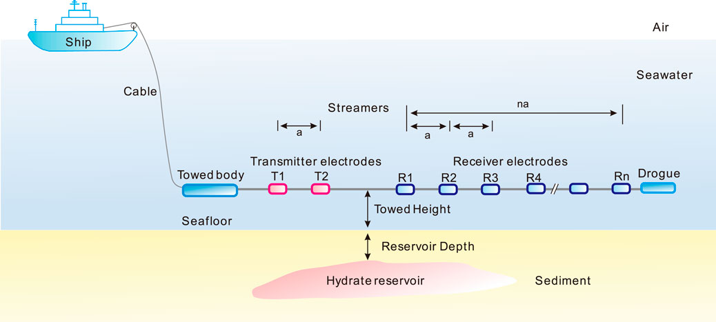
FIGURE 1. Configuration of marine towed electrical resistivity system with multi-component streamers DCR array arrangement. The ship towed a long cable close to the seafloor to detect structures beneath the seafloor. The DCR array arrangement is composed of multiple receiver electrodes along with transmitter electrodes, and the number of the receiver electrodes is more than that of the transmitter electrodes. The effect of exploration can be perfected by increasing the quantity of the receiver electrodes in the DCR array arrangement.

A variety of DCR array arrangements are available: the pole electrical dipole, the vertical electrical dipole, the horizontal electrical dipole, and the rest.

But, the horizontal array measurement proves to be more convenient and quicker compared with the vertical array in the marine environment. Meanwhile, the reservoir is generally characterized by a horizontal distribution, while the horizontal array represents more sensitivity to such a horizontal distribution structure. Therefore, this paper is based on the use of horizontal array measurement.

The DCR reveals the resistivity structure by injecting current into the transmitter electrodes on the cable and gauging the potential difference at the receiver electrodes. The apparent resistivity is confirmed via the equation below:

${\rho }_a=\text{k}\frac{V}{I}(1)$

Where ${\rho }_a$: apparent resistivity, k: array geometric coefficient, V: electric potential, I: electric current. The geometric factors of the device are defined as the quasi-space containing conductive seawater and seafloor. The horizontal array includes: Inline dipole-dipole, Wenner-Schlumberger, Wenner-Alpha (Figure2).

FIGURE 2

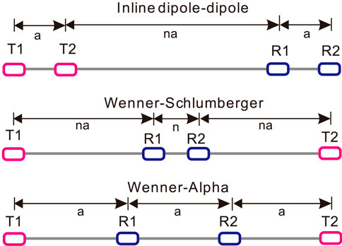
FIGURE 2. The electrodes arrangement of various DCR array arrangements.

The geometric factors are derived from the following equations:

$k=2\text{πn}\left(\text{n}+1\right)(\text{n}+2)\text{a}(\mathrm{2a})$

$k=2\text{πn}\left(\text{n}+1\right)\text{a}(\mathrm{2b})$

$k=4\text{πa}(\mathrm{2c})$

Where a: the spacing between the receiver electrodes, n: number of the receiver electrodes interval.

The method used for the grid construction of the synthetic model in this paper is the finite difference method (FDM), which adopts a two-dimensional model with a rectangular grid to divide the subsurface into several blocks. The finite difference method basically determines the potentials of the nodes of the rectangular grid, which consists of nodes in the horizontal direction and nodes in the horizontal direction. These blocks can have different resistivity values. By using a sufficiently fine grid, complex geological structures can be modeled.

2.2 Resistivity inversion

The inversion of the resistivity solves a nonlinear optimization problem with ill-posed and non-unique characteristics. The regularization of this problem is by working out the following function (Gundogdu and Candansayar, 2018):

${\text{P}}^{\text{α}}\left(\text{m},\text{d}\right)=\varphi \left(\text{m},\text{d}\right)+\text{αS}\left(\text{m}\right)(3)$

where ϕ(m,d): misfit function, S(m): stabilization function, and α: regularization parameter. The misfit function as follows:

$\mathrm{\varphi }\left(\text{m},\text{d}\right)={\displaystyle {\sum }_{\text{i}=1}^{\text{N}}{\left({\text{d}}_{\text{i}}-{\text{f}}_{\text{i}}\left(\text{m}\right)\right)}^2}=\parallel \text{d}-\text{f}{(\text{m})\parallel }_2^2(4)$

The misfit function is the distance between the measured data d_i and the calculated data $f_i\left(m\right)$. A weighting factor is specified to ensure that the measured data with noise has less effect on the results.

$\mathrm{\varphi }\left(\text{m},\text{d}\right)=\parallel {\text{W}}_{\text{d}}{(\text{d}-\text{f}\left(\text{m}\right))\parallel }_2^2(5)$

where $W_d$: data weighting matrix. The weighted stabilization function is as follows:

${\text{S}}_{\text{w}}\left(\text{m}\right)={\text{W}}_{\text{m}}\text{S}\left(\text{m}\right)(6)$

where $W_m$: sensitivity model weighting function. The pseudo-quadratic form of the stabilization function can be written as follows (Candansayar, 2008):

${\text{S}}_{\text{w}}\left(\text{m}\right)=\parallel {\text{W}}_{\text{e}}{\text{W}}_{\text{m}}{\text{m}\parallel }^2(7)$

where $W_e$: the linear operator of model parameters. The stabilization function defined in this way allows different stabilizers to be inserted into the inversion algorithm. The Gauss-Newton least square method is commonly used for resistivity inversion (Oldenburg and Li, 1994).

Moreover, the fitting error method aims to reduce the discrepancy between the calculated and measured values. In this study, it is done by adjusting the resistivity of the model block to minimize the difference between the calculated and measured values. The measure of this discrepancy is given by the root mean square error (RMS). In general, the most prudent approach is to select the model in iterations where the RMS error does not change significantly after the iteration to obtain the best inversion results. This usually occurs between the third and sixth iterations, and in this paper, 20 iterations were done to demonstrate the convergence of the iterations. RMS calculation equation is as follows:

$RMS=\sqrt{\frac{{\displaystyle \sum _{i=1}^n{\left(X_{c,i}-X_{m,i}\right)}^2}}{n}}(8)$

where $X_{c,i}$: calculated values, $X_{m,i}$: measured values.

2.3 Hydrate saturation

Gas hydrate saturation is a critical parameter for gas hydrate study. The resistivity can be used to evaluate hydrate’s porosity and saturation. The empirical equation of saturation can be determined according to the drilling core and logging data. Lee and Collett (2006) discussed the effectiveness of argillaceous parameter correction on the estimation of hydrate saturation. Schwalenberg et al. (2020) used the correction equation with an argillaceous parameter to estimate the hydrate saturation in the Black sea. Liu et al. (2017) compared the difference between the traditional Archie equation and the empirical correction equation, compared the theoretical value of saturation calculated by the two equations with the actual value obtained by drilling, and found that the resistivity method with clay correction can accurately predict hydrate saturation.

The Archie’s equation is used to calculate water saturation in the marine sediment (Archie, 1942). In the reservoir, the filling of the sedimentary layer can be approximately regarded as the filling of gas hydrate and seawater. The equation is as follows:

$S_{gh}=1-S_w(9)$

where $S_{gh}$: the gas hydrate saturation, $S_w$ : the saturation of water. Archie’s equation is as follows (Archie, 1942):

$S_w={\left(\frac{a{\rho }_{\omega }}{{\phi }^m{\rho }_f}\right)}^{\frac{1}{n}}(10)$

where a: the parameter related to lithology, ${\rho }_{\omega }$: the resistivity of water, φ: the porosity, m: the cementation index, ${\rho }_f$: the resistivity of sedimentary layer, n: the saturation index. The values of a and m are associated with each other, and their selection has been widely discussed in the literature (Jackson et al., 1978). According to the sample data reported in previous literature, it can be known that in the natural gas hydrate reservoir, the average value of n is 1.9386 (Pearson et al., 1983). For a variety of rock samples, the value of n is different. The value of φ is related to rock samples. The calculation equation of gas hydrate saturation can be defined as follows:

$S_{gh}=1-{\left(\frac{a{\rho }_{\omega }}{{\phi }^m{\rho }_f}\right)}^{\frac{1}{n}}(11)$

The presence of clay affects the sediment resistivity and Archie coefficient, leading to incorrect saturation estimation. The saturation calculation equation of natural gas hydrate with argillaceous clay can be modified as follows (Lee and Collett, 2006):

$S_{gh}=1-{\left(\frac{a{\rho }_{\omega }\left(1-{\rho }_f{Q}_c\right)}{{\phi }^m{\rho }_f}\right)}^{\frac{1}{n}}(12)$

Where $Q_c$: the effective resistivity of clay. The equation is as follows:

$Q_c=\frac{{\mathit{V}}_c\left(1-\phi \right)}{R_c}(13)$

Where, $V_c$: the volume content of argillaceous clay, $R_c$: the resistivity of argillaceous clay. Figure 3 shows the hydrate saturation variation with resistivity calculated using the above conventional and corrected equations.

FIGURE 3

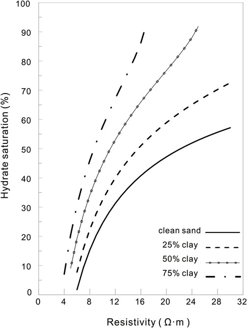
FIGURE 3. The curve of the hydrate saturation varying in depth is suitable for natural gas hydrate reservoirs with various clay content.

The saturation estimated by the modified equation is slightly higher than that estimated by the conventional equation. For example, when the resistivity is 30 Ω m, the saturation is 15 Ω m higher than that estimated by the conventional equation.

Since the reservoir is included in the background formation and seawater in the resistivity inversion results, these backgrounds need to be excluded from the calculation in the saturation calculation. We have derived the resistivity conversion equation from reservoir saturation from Eq. 12 to determine the critical value of resistivity when reservoir saturation is 0. The equation is shown as follows:

${\rho }_f=\frac{1}{Q_c+\frac{{\phi }^m{\left(1-S_{gh}\right)}^n}{a{\rho }_{\omega }}}(14)$

where $S_{gh}$: the gas hydrate saturation, φ: the porosity, m: the cementation index, ${\rho }_f$: the resistivity of sedimentary layer, n: the saturation index, $Q_c$: the effective resistivity of clay. That the critical value of resistivity of reservoir saturation 0 using Eq. 14 is 5.2154 Ω m after calculation.

Previous studies have found that the complexity of the physical properties of marine sediments may lead to changes in the parameters of the Archie equation. Lee and Collett (2006) discussed the effect of clay percentage content on a and m values using the downhole resistivity from logging data. Guo et al. (2021) studied the penetration resistance coefficient of marine sediment clay.

The actual situation should take into consideration using the Archie equation with parameter correction, as shown in Table 1. It can be seen that the higher the content of argillaceous clay, the greater the a value and the smaller the m value. The clay content can usually be determined according to the physical parameters of the drilling core.

TABLE 1

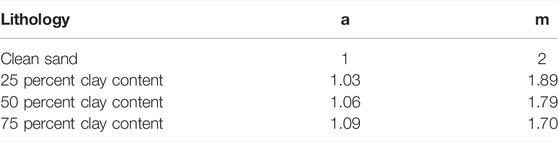
TABLE 1. Comparison between argillaceous clay content and a and m value (Lee and Collett, 2006).

Figure 3 shows the hydrate saturation curve with the reservoir’s depth with various clay content (Lee and Collett, 2006) (Table 1).

The clay content will affect the calculated saturation. The calculated saturation will increase as clay content mounts.

In terms of the same resistivity, the higher the clay content of the reservoir, the higher the saturation of gas hydrate. When evaluating the occurrence state of natural gas hydrate, it is necessary to conduct drilling sampling, investigate the lithology of marine sediments, and then select appropriate correction parameters.

3 Results and discussion

The resistivity inversion and saturation estimation are evaluated from eight aspects by synthetic model calculation: (1) the DCR array arrangement; (2) the towed height of the instruments away from the seafloor; (3) the buried depth at the top of the reservoir; (4) the length of gas hydrate reservoir; (5) the thickness of gas hydrate reservoir; (6) the tilt of gas hydrate reservoir; (7) the horizontal resolution; (8) the vertical resolution

3.1 Comparison of various DCR array arrangement

We have compared the resistivity inversion and the hydrate saturation to the synthetic models with various marine towed DCR array arrangements: Inline dipole-dipole, Wenner-Schlumberger, Wenner-Alpha.

3.1.1 Model parameters

Various DCR array arrangements that need to be compared in this group of models is shown in Table 2.

TABLE 2

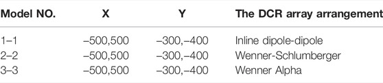
TABLE 2. The model parameters of various DCR array arrangements that need to be compared in this group.

In this group of models, the electrode spacing a is 25m, and the isolation coefficient n is 8.

The buried depth at the top of the reservoir is 100 m; the length of the reservoir is 1000 m; the thickness of the reservoir is 100 m; the resistivity of the reservoir is 20 Ω·m; the resistivity of marine sediments is 5 Ω·m; the resistivity of seawater is 0.33 Ω·m; and the total length of the survey line is 5,000 m. The arrangements in this synthetic model are: Inline dipole-dipole, Wenner-Schlumberger, Wenner-Alpha.

3.1.2 Results

The resistivity inversion and hydrate saturation estimation of various array models (Model 1–1, 1-2, and 1–3) are displayed in Figure 4D-I, respectively. The high resistivity range and the high saturation range obtained by the resistivity inversion are consistent with the synthetic model’s reservoir range.

FIGURE 4

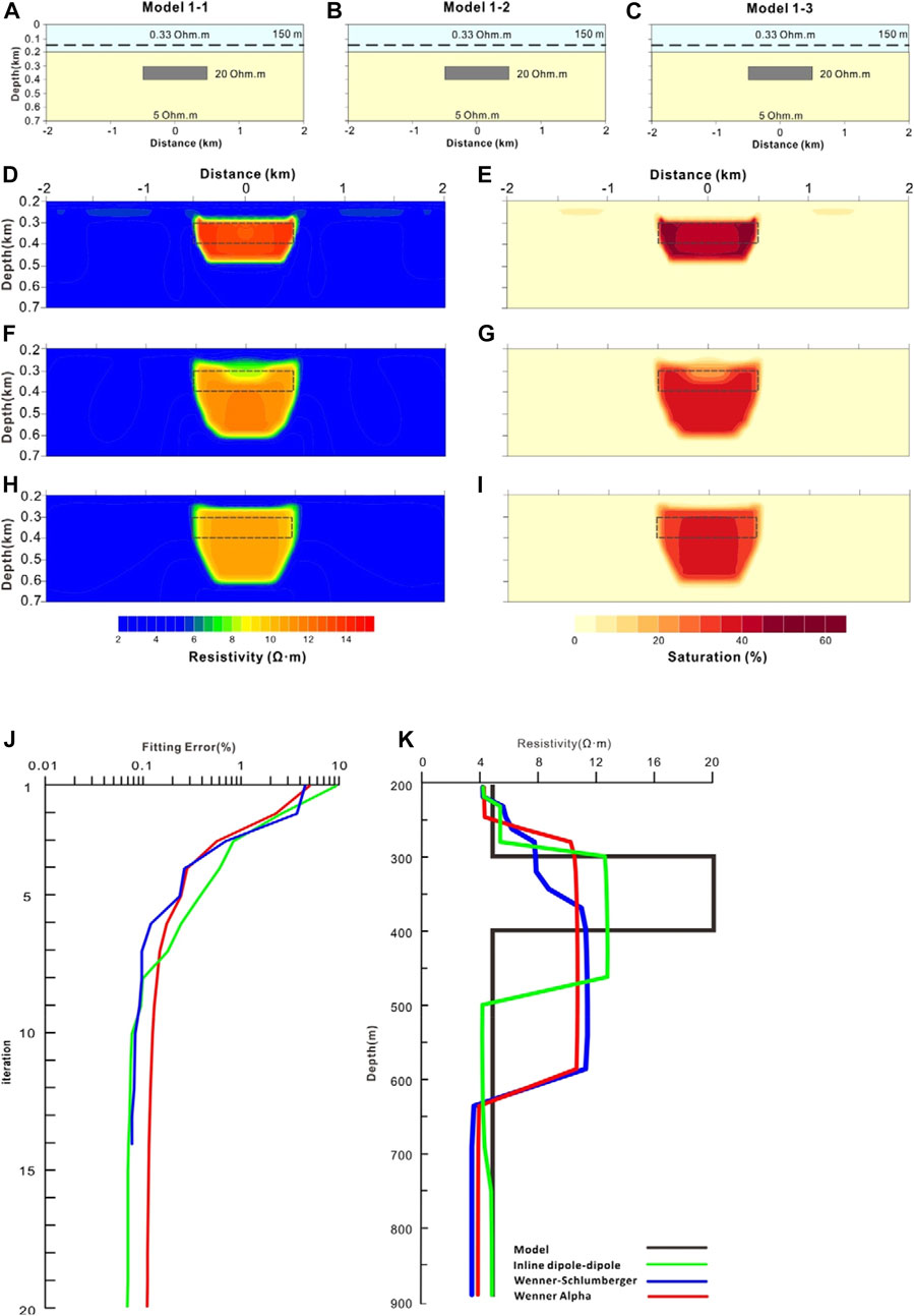
FIGURE 4. Resistivity inversion and hydrate saturation estimation of variable array model. (A)–(C): In the schematic diagram of Model 1–1, 1-2, and 1-3 respectively, light blue indicates seawater, light yellow indicates marine sediments, gray block indicates hydrate reservoirs, dotted line indicates the track of the towed resistivity array; (D), (F) and (H): the inversion resistivity of Model 1–1, 1-2, and 1-3 respectively; (E), (G) and (I): the hydrate saturation of Model 1–1, 1-2, and 1-3 respectively (J): the inversion iteration convergence of Model 1–1(green), 1–2(blue) and 1–3 (red), respectively (K): the resistivity profile with depth at the center x position of hydrate reservoir of Model 1–1(green), 1–2(blue) and 1–3 (red), respectively.

The depth of the high resistivity area also basically corresponds to the depth range of the hydrate reservoir (300–400 m). However, there are still slight differences in the inversion results of these various array arrangements (Model 1–1, 1-2, and 1–3). Among them, the inversion of the Inline dipole-dipole array arrangement (Model 1–1) is 300–470 m, and the depth range of high resistivity area obtained from the inversion results of the Wenner-Schlumberger and the Wenner-Alpha array arrangement (Model 1-2, and 1–3) are 370–590 m and 280–59 m, respectively.

The inversion iteration convergence of Model 1–1, 1–2, and 1–3 are shown in Figure 4J. The RMS fitting errors of the inversion iteration for all array arrangements have converged below 0.1%, which meets the requirements of inversion accuracy.

We have extracted the resistivity curve of the central position of the hydrate reservoir with depth from the inversion resistivity results, so as to intuitively see the variation of gas hydrate resistivity with depth (Figure 4K). The resistivity value of the hydrate reservoir varies from 10 to 13 Ω·m in the resistivity inversion results and the anomalies of submarine gas hydrate are reflected in various accuracy.

3.1.3 Discussion

In the curve of the resistivity value compared with the truth resistivity, it can be seen that when the electrode arrangement is an Inline dipole-dipole array arrangement, the calculated resistivity anomaly is closest to the model resistivity anomaly, and the calculated resistivity anomaly range matches the model resistivity anomaly range the best. Therefore, Inline dipole-dipole array arrangement has the highest accuracy.

The results show that the reservoir position obtained by inversion imaging with three conventional array arrangements is in good agreement with the real model. The inversion effect of the Inline dipole-dipole array agrees best with the real model. The inversion from the other two array arrangements (Wenner-Schlumberger, Wenner-Alpha) has a relatively large deviation in the vertical position of the reservoir.

The imaging recognition of the upper boundary of the reservoir with these three array arrangements is generally more accurate than that of the lower boundary. It is inferred that DCR is better for shallow reservoir identification than deep reservoir identification. The resolution of the dipole-dipole array in marine towed DC imaging of hydrate is better than that of the Wenner array.

In addition, the transmitter electrodes are the dipole-dipole array is located on both sides of the towing cable. The front section of the cable is equipped with the transmitter electrodes, and the tail end can then be flexibly configured with the number of the receiver electrodes and transceiver offset distance as required. These have higher data acquisition efficiency in the actual construction of offshore surveys, so we believe that the use of an Inline dipole-dipole array is more suitable for hydrate reservoir exploration.

3.2 Comparison of various towed height

We have compared the inversion results of the resistivity inversion and the hydrate saturation to the synthetic models with various towed heights.

3.2.1 Model parameters

The model parameters of the various towed heights of the array arrangement away from the seafloor is shown in Table 3.

TABLE 3

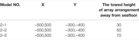
TABLE 3. The model parameters of the various towed heights of the array arrangement away from the seafloor that need to be compared in this group.

In this group of models, the array arrangement of Inline dipole-dipole is used, the electrode spacing a is 25 m, and the isolation coefficient n is 8.

The buried depth of the reservoir is 100 m; the length of the reservoir is 1000 m; the thickness of the reservoir is 100 m; the resistivity of the reservoir is 20 Ω m; the resistivity of marine sediments is 5 Ω·m; the resistivity of seawater is 0.33 Ω·m; and the total length of the survey line is 5,000 m. The towed height in this group is 30, 50, and 70 m, respectively.

3.2.2 Results

The resistivity inversion and hydrate saturation estimation of the variable array arrangement model (Model 2–1, 2-2, and 2–3) are shown in Figure 5D-I, respectively. The high resistivity range and the high saturation range obtained by the resistivity inversion are basically consistent with the reservoir range in the synthetic model. The resistivity value of the hydrate reservoir varies from 12 to 18 Ω·m in the resistivity inversion results and the anomalies of submarine gas hydrate are reflected with different accuracy.

FIGURE 5

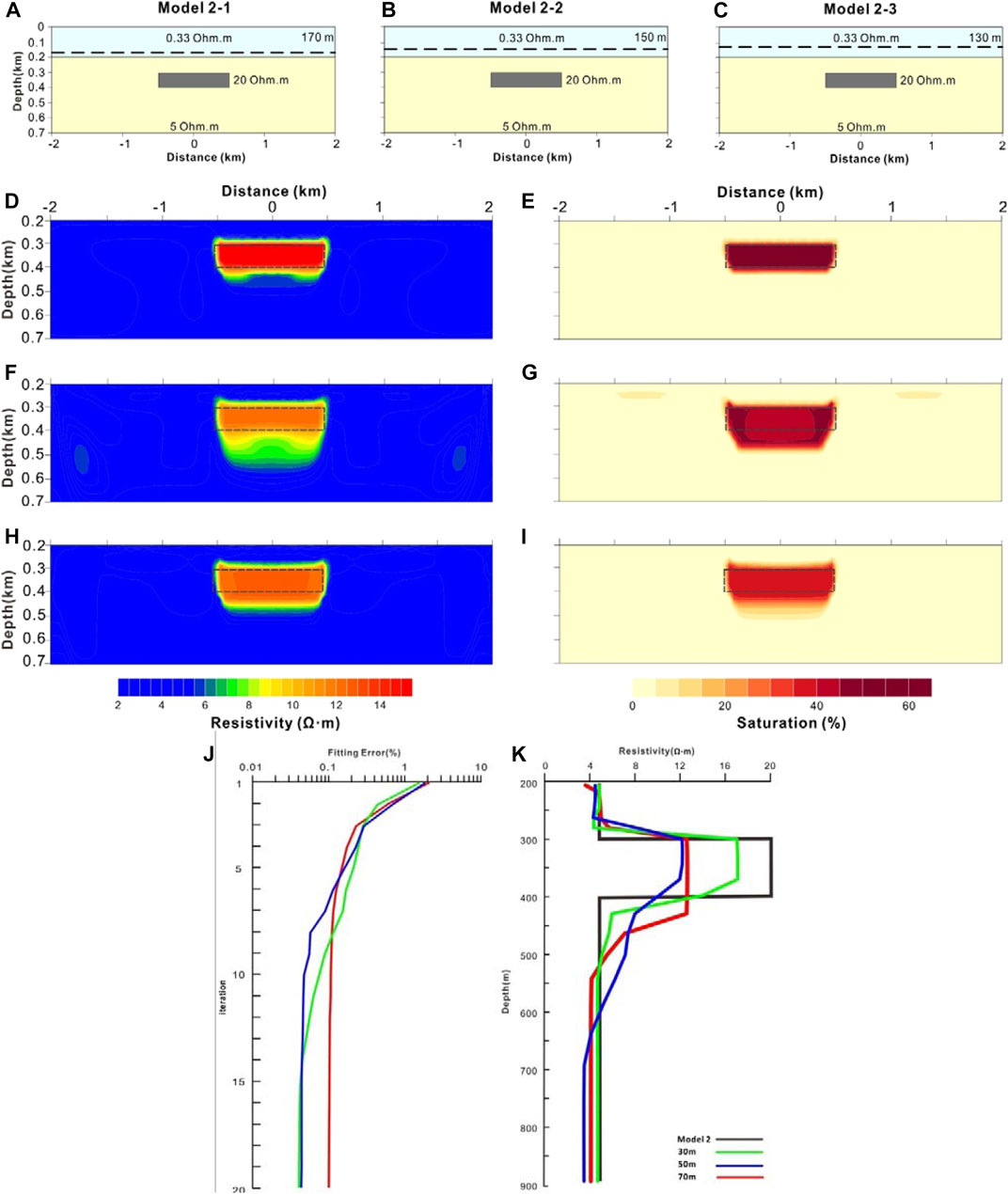
FIGURE 5. Resistivity inversion and hydrate saturation estimation of variable towed height model of the array arrangement away from the seafloor. (A)–(C): In the schematic diagram of Model 2–1, 2-2, and 2-3 respectively, light blue indicates seawater, light yellow indicates marine sediments, gray block indicates hydrate reservoirs, dotted line indicates the track of the towed DCR array arrangement; (D), (F) and (H): the inversion resistivity of Model 2–1, 2-2, and 2-3 respectively; (E), (G) and (I): the hydrate saturation estimation of Model 2–1, 2-2, and 2-3 respectively (J): the inversion iteration convergence of Model 2–1(green), 2–2(blue) and 2–3 (red), respectively (K): the resistivity profile with depth at the center x position of hydrate reservoir of Model 2–1(green), 2–2(blue) and 2–3 (red), respectively.

The depth of the high resistivity area also basically corresponds to the depth range of the hydrate reservoir (300–400 m). However, there are still slight differences in the inversion results of these various array arrangements. Among them, the inversion of the towed height 30 and 50 m (Model 2-1 and 2–2) is 300–370 m, and the depth range of high resistivity area obtained from the inversion results of the towed height of 70 m (Model 2–3) are 300–425 m.

The inversion iteration convergence of the towed height 30, 50, and 70 m (Model 2–1, 2–2, and 2–3) are shown in Figure 5J. The fitting error of the inversion iteration for Model 2–1 and 2–2 has converged below 0.1% after the 8th and 12th iterations, which meets the requirements of inversion accuracy. The fitting error of the inversion iteration for Model 2–3 has decreased rapidly after eight iterations and then maintained at about 0.17% through many iterations, which also meets the inversion accuracy.

We have extracted the resistivity curve of the central position of the hydrate reservoir with depth from the inversion resistivity imaging map, so as to intuitively see the variation of gas hydrate resistivity in depth (Figure 5K). The resistivity value of the hydrate reservoir varies from 12 to 17 Ω·m in the resistivity inversion results and the anomalies of submarine gas hydrate are reflected with various accuracy.

3.2.3 Discussion

From the comparison between the inversion and the truth resistivity, it can be seen that when the towing height is 30 m, the inversion resistivity of the reservoir is the closest to the truth. Moreover, the accuracy of inversion results increases with the decrease of towing altitude. When the towing height is 30 m, the inversion reservoir thickness is about 100 m and the reservoir resistivity is 16 Ω·m, which is the closest to the truth resistivity (Figure 5K).

The inversion becomes better with the decrease of towing height. The inverted reservoir boundary is closer to the truth. Seawater is a good conductor compared with marine sediments. When electrical methods are used in the marine environment, seawater has a strong attraction to current. If the measurement is too far from the seabed, the emitted current may rarely penetrate the seabed sediments, and the signal from the deep seabed is very weak. This is unfavorable for the inversion of highly resistive reservoirs in marine sediments.

3.3 Comparison of various reservoir depth

We have compared the inversion results of the resistivity inversion and the hydrate saturation to the synthetic models with the various buried depths of the reservoir.

3.3.1 Model parameters

Various buried depths at the top of the hydrate reservoir of the reservoir need to be compared in this group is shown in Table 4.

TABLE 4

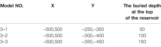
TABLE 4. The model parameters of various buried depth at the top of the reservoir that needs to be compared.

In this group of models, the array arrangement of Inline dipole-dipole is employed, the electrode spacing a is 25 m, and the isolation coefficient n is 8.

The length of the reservoir is 1000 m; the thickness of the reservoir is 100 m; the resistivity of the reservoir 20 Ω·m; the resistivity of marine sediments is 5 Ω·m; the resistivity of seawater is 0.33 Ω·m; and the length of the survey line is 5,000 m. The buried depth at the top of the reservoir in this group is 50, 100, and 150 m, respectively.

3.3.2 Results

The resistivity inversion and hydrate saturation estimation of variable buried depth at the top of the reservoir (Model 3–1, 3–2, and 3–3) are shown in Figure 6D-I, respectively. The high resistivity range and the high saturation range obtained by the resistivity inversion are consistent with the synthetic model’s reservoir range.

FIGURE 6

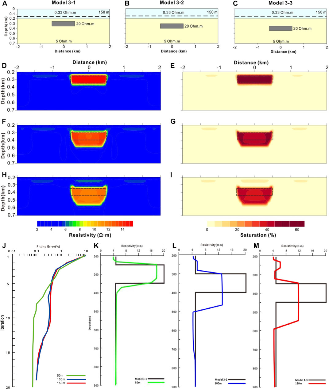
FIGURE 6. Resistivity inversion and hydrate saturation estimation of various buried depths at the top of the reservoir. (A)–(C): the schematic diagram of Model 3–1, 3-2, and 3-3 respectively, light blue indicates seawater, light yellow indicates marine sediments, gray block indicates hydrate reservoirs, dotted line indicates the track of the towed DCR array; (D), (F) and (H): the inversion resistivity of Model 3–1, 3-2, and 3-3, respectively; (E), (G) and (I): the hydrate saturation of Model 3–1, 3–2, and 3–3, respectively (J): the inversion iteration convergence of Model 3–1(green), 3–2(blue) and 3–3 (red), respectively (K)–(M): the resistivity profile with depth at the center x position of hydrate reservoir of Model 3–1(green), 3–2(blue) and 3–3 (red), respectively.

The depth of the high resistivity area basically corresponds to the depth range of the hydrate reservoir. However, there are still differences in the inversion results of these different models. Among them, the inversion depth of the hydrate reservoir in Model 3–1 (50–120 m) was closest to the truth (50–150 m). The inversion depth of the hydrate reservoir in Model 3–2 (100–270 m) was closer to the truth (100–200 m). The inversion depth of the hydrate reservoir in Model 3–3 (150–350 m) basically corresponded to the true depth (150–250 m).

The inversion iteration convergence of the buried depth 50, 100, and 150 m (Model 3–1, 3-2, and 3–3) are shown in Figure 6 (j). The RMS fitting errors of all model calculation results have met the convergence requirements. However, the inversion fitting in Model 3-1 was the best of all models. The fitting error reached 0.1% in the 8th iteration and remained at about 0.07% after the 10th iteration in Model 3–1. The fitting in Model 3-2, and Model 3-3 is poor, and their fitting error converges to 0.1% at the 18th iteration.

We have extracted the resistivity curve of the central position of the hydrate reservoir with depth from the inversion resistivity imaging map, so as to intuitively apprehend the variation of gas hydrate resistivity in depth (Figure 6K-M). The resistivity value of the hydrate reservoir varies from 12 to 19 Ω m in the resistivity inversion results and the anomalies of submarine gas hydrate are reflected with different accuracy.

3.3.3 Discussion

From the comparison between the inversion and the true resistivity, it can be seen that when the reservoir depth is 50 m, the inversion resistivity of the reservoir is the closest to the truth. Moreover, the accuracy of inversion results increases as the reservoir depth increases. When the reservoir size is fixed and the reservoir depth becomes larger, the distribution range of the inversion reservoir will be excessively expanded and the resistivity value will be underestimated (Figure 6K-M).

Therefore, it is suggested that when using DCR to detect marine hydrate reservoirs, the true range may be smaller than the inversion result after the reservoir depth increases. We suggest increasing the electrode distance of the detection device, the distance between the transmitting and receiving electrodes, and the intensity of the emitted current to improve the detection effect of deep reservoirs.

3.4 Comparison of various reservoir lengths

We have compared the inversion results of the resistivity inversion and the hydrate saturation to the synthetic models with various lengths of the reservoir.

3.4.1 Model parameters

The location of various lengths of hydrate reservoir that need to be compared in this group is shown in Table 5.

TABLE 5

TABLE 5. The model parameters of various lengths of the reservoir that need to be compared in this group.

In this group of models, the array arrangement of Inline dipole-dipole is used, the electrode spacing a is 25 m, the isolation coefficient n is 8, and the towed height is 30 m. The buried depth at the top of the reservoir is 100 m; the thickness of the reservoir is 100 m; the resistivity of the reservoir is 20 Ω m; The resistivity of marine sediments is 5 Ω·m; the resistivity of seawater is 0.33 Ω·m; the length of the survey line is 5,000 m. The length of the reservoir in this group is 500, 1000, and 1500 m, respectively.

3.4.2 Results

The resistivity inversion and hydrate saturation estimation of various length models of gas hydrate reservoir (Model 4–1, 4–2, and 4–3) are shown in Figure 7D-I, respectively. The high resistivity range and the high saturation range obtained by the resistivity inversion are basically consistent with the reservoir range in the synthetic model.

FIGURE 7

FIGURE 7. Resistivity inversion and hydrate saturation estimation of the various length model of hydrate reservoir. (A)–(C): the schematic diagram of Model 4–1, 4-2, and 4-3 respectively, light blue indicates seawater, light yellow indicates marine sediments, gray block indicates hydrate reservoirs, dotted line indicates the track of the towed DCR array arrangement; (D), (F) and (H): the inversion resistivity of Model 4–1, 3–2, and 4-3 respectively; (E), (G) and (I): the hydrate saturation estimation of Model 4–1, 4–2, and 4-3 respectively (J): the inversion iteration convergence of Model 4–1(green), 4–2(line) and 4–3 (red), respectively (K): the resistivity profile with depth at the center x position of hydrate reservoir of Model 4–1(green), 4–2(blue) and 4–3 (red), respectively.

The length of the high resistivity area basically corresponds to the length range of the reservoir. However, there are still differences in the inversion results of these different models. Among them, the inversion buried depth the reservoir in Model 4–1 (100–220 m) was closest to the truth (100–200 m). The inversion buried depth of the reservoir in Model 4–2 (100–220 m) was closer to the truth (100–200 m). The inversion buried depth of the reservoir in Model 4–3 (100–290 m) basically corresponds to the truth (150–200 m).

The inversion iteration convergence of the reservoir length 500 m, 1000 m, and 1500 m (Model 4–1, 4-2, and 4–3) are shown in Figure 7J. The RMS fitting errors of all model calculation results have met the convergence requirements. However, the inversion fitting in Model 4-1 reached 0.1% in the 8th iteration and remained at about 0.07% after the 12th iteration. The fitting error in Model 4-2, and Model 4-3 converged to 0.1% at the 15th iteration.

We have extracted the resistivity curve of the central position of hydrate reservoir with depth from the inversion resistivity imaging map, so as to intuitively see the variation of gas hydrate resistivity with depth (Figure 7K). The resistivity value of the hydrate reservoir varies from 12 to 17 Ω·m in the resistivity inversion results and the anomalies of submarine gas hydrate are reflected with various accuracy.

3.4.3 Discussion

From the comparison between the inversion and the truth resistivity, it can be seen that when the reservoir length is 500 m, the inversion resistivity of the reservoir is the closest to the truth. Moreover, the accuracy of inversion results increases with the decrease of the reservoir length. Model 4–1, 4–1 and 4–3 accurately identify reservoir distribution by resistivity inversion, including reservoir thickness and length (Figure 7). When the reservoir thickness is fixed and the reservoir length becomes shorter, the resistivity of the reservoir will increase, especially in the minimum reservoir length model (Model 4–1).

The actual range may be smaller than the inversion result of DCR detecting marine hydrate reservoirs when the reservoir depth increases. DCR can detect hydrate reservoirs with various lengths. It is necessary to ensure that the survey line covers the extension of the reservoir for exploration.

3.5 Comparison of various reservoir thickness

We have compared the inversion results of the resistivity inversion and the hydrate saturation to the synthetic models with various thicknesses of the reservoir.

3.5.1 Model parameters

Various thicknesses of hydrate reservoir that need to be compared in this group is shown in Table 6.

TABLE 6

TABLE 6. The model parameters of various thicknesses of hydrate reservoir that need to be compared in this group.

In this group of models, the array arrangement of the Inline dipole-dipole is used, the electrode spacing a is 25 m, the isolation coefficient n is 8, and the towed height is 30 m. The length of the hydrate reservoir is 1000 m; the thickness of the reservoir 100m; the buried depth at the top of the reservoir is 100 m; the resistivity of the reservoir is 20 Ω·m; the resistivity of marine sediments is 5 Ω·m; the resistivity of seawater 0.33 Ω·m The length of the survey line 5,000 m. The thickness of the hydrate reservoir in this group is 100, 150, and 200 m, respectively.

3.5.2 Results

The resistivity inversion and hydrate saturation estimation of various thickness models of gas hydrate reservoirs (Model 5–1, 5-2, and 5–3) are shown in Figure 8D-I, respectively. The high resistivity range and the high saturation range obtained by the resistivity inversion are basically consistent with the reservoir range in the synthetic model.

FIGURE 8

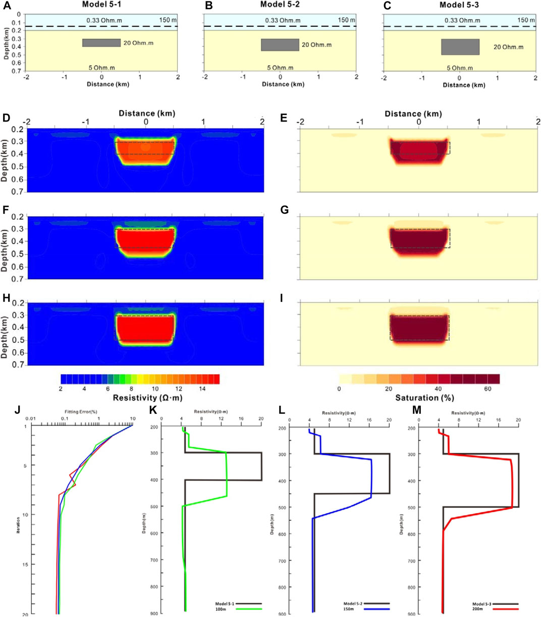
FIGURE 8. Resistivity inversion and hydrate saturation estimation of various thickness models of hydrate reservoir. (A)–(C): the schematic diagram of Model 5–1, 5–2, and 5–3 respectively, light blue indicates seawater, light yellow indicates marine sediments, gray block indicates hydrate reservoirs, dotted line indicates the track of the towed DCR array arrangement; (D), (F) and (H): the inversion resistivity of Model 5–1, 3–2, and 5–3 respectively; (E), (G) and (I): the hydrate saturation estimation of Model 5–1, 5–2, and 5–3 respectively (J)d: the inversion iteration convergence of Model 5–1(green), 5–2(blue) and 5–3 (red), respectively (K)–(M): the resistivity profile with depth at the center x position of hydrate reservoir of Model 5–1(green), 5–2(blue) and 5–3 (red), respectively.

The depth of the resistivity area basically corresponds to the depth range of the hydrate reservoir. However, there are still differences in the inversion results of these different models. Among them, the inversion thickness of the hydrate reservoir in Model 5–3 (220 m) was closest to the model thickness (200 m). The inversion thickness of the hydrate reservoir in Model 5–2 (170 m) was closer to the model thickness (150 m). The inversion buried depth at the top of the reservoir in Model 5–1 (170 m) basically corresponds to the truth (100 m).

The iteration convergence of the inversion (Model 5–1, 5-2, and 5–3) is shown in Figure 8J. The RMS fitting errors of all model calculation results have met the convergence requirements. The RMS fitting errors in all models were converged to 0.1% at the eighth iteration.

We have extracted the resistivity curve of the central position of the hydrate reservoir with depth on the inversion resistivity imaging map, so as to intuitively see the variation of gas hydrate resistivity in depth (Figure 8K-M). The resistivity value of the hydrate reservoir varies from 14 to 19 Ω·m in the resistivity inversion results and the anomalies of submarine gas hydrate are reflected with different accuracy.

3.5.3 Discussion

From the comparison between the inversion and the truth resistivity, it can be seen that when the reservoir thickness is 200 m (Model 5–3), the inversion resistivity of the reservoir is the closest to the truth. The range of inversion resistivity is the best match with that of the truth. Moreover, the accuracy of inversion results increases with the increase of the reservoir thickness. When the reservoir length is fixed and the reservoir thickness becomes thicker, the resistivity of the reservoir will increase, especially in the thickest reservoir model (Model 5–3) (Figure 8).

DCR can detect hydrate reservoirs of various thicknesses. When the reservoir thickness increases, the inversion is in good agreement with the truth, which indicates that this method can identify thicker reservoirs.

3.6 Comparison of various reservoir tilt

We have compared the inversion results of the resistivity inversion and the hydrate saturation to the synthetic models with various dips in the hydrate reservoir.

3.6.1 Model parameters

The location of various tilts of the reservoir that need to be compared in this group is shown in Table 7.

TABLE 7

TABLE 7. The model parameters of various dips of the hydrate reservoir that need to be compared in this group.

In this group of models, the DCR array arrangement of the Inline dipole-dipole is used, the electrode spacing a is 25 m, the isolation coefficient n is 8, and the towed height is 30 m. The length of the reservoir is 1000 m; the thickness of the reservoir 100 m; the buried depth at the top of the reservoir is 100 m; the resistivity of the reservoir is 20 Ω·m; the resistivity of marine sediments is 5 Ω·m; the resistivity of seawater is 0.33 Ω·m; the length of the survey line is 5,000 m. The tilt of the hydrate reservoir in this group is 0 and 45, respectively.

3.6.2 Results

The resistivity inversion and hydrate saturation estimation of various dip models of hydrate reservoir (Model 6-1 and 6–2) are shown in Figure 9D-I, respectively. The high resistivity range and the high saturation range obtained by the resistivity inversion are basically consistent with the reservoir range in the synthetic model. The effect of the model of the reservoir tilt = 0 (Model 6–1) is the best.

FIGURE 9

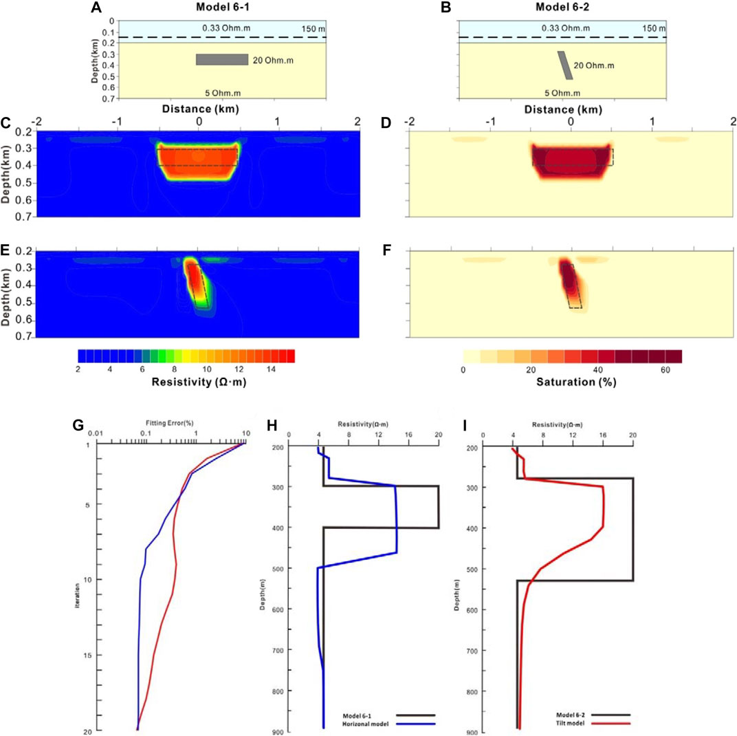
FIGURE 9. Resistivity inversion and hydrate saturation estimation of the various thickness model of hydrate reservoir. (A)–(B): the schematic diagram of Model 6-1 and 6-2 respectively, light blue indicates seawater, light yellow indicates marine sediments, gray block indicates hydrate reservoirs, dotted line indicates the track of the towed DCR array arrangement; (C) and (I) the inversion resistivity of Model 6-1and 6-2 respectively; (D) and (F): the hydrate saturation estimation of Model 6-1 and 6-2 respectively; (G): the inversion iteration convergence of Model 6–1 (blue) and 6–2 (red), respectively; (H)–(I): the resistivity profile with depth at the center x position of hydrate reservoir of Model 6–1 (blue) and 6–2 (red), respectively.

The depth of the resistivity area basically corresponds to the depth range of the hydrate reservoir. However, there are still variations in the inversion results of these models.

The distribution inversion of the reservoir dip = 0 (Model 6–1) is the best among them. The inversion iteration convergence of the reservoir dip = 0, 45 (Model 6−1 and 6–2) are shown in Figure 9G. The RMS fitting errors of all model calculation results have met the convergence requirements.

We have extracted the resistivity curve of the central position of the hydrate reservoir with depth on the inversion resistivity imaging map, so as to intuitively see the variation of gas hydrate resistivity in depth (Figure 9H-I). The resistivity value of the hydrate reservoir varies from 12 Ω.m in the resistivity inversion results and the anomalies of submarine gas hydrate are reflected with various accuracy.

3.6.3 Discussion

From the comparison between the inversion and the truth resistivity, it can be seen that the inversion of the tilt model is consistent with the truth. This method can identify the reservoirs with inclined conditions, but horizontal reservoirs are better in terms of their inversion effect.

3.7 Horizontal resolution

We have compared the resistivity inversion and the hydrate saturation with the numerical horizontal distribution combination model, which is to evaluate the ability to distinguish two different reservoirs in the horizontal distribution.

3.7.1 Model parameters

The location of various horizontal distribution combination models of hydrate reservoirs that need to be compared in this group is shown in Table 8. In this group of models, the DCR array arrangement of Inline dipole-dipole is used, the electrode spacing a is 25 m, the isolation coefficient n is 8, and the towed height is 30 m.

TABLE 8

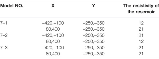
TABLE 8. The model parameters of various horizontal distribution combination models of hydrate reservoirs that need to be compared in this group.

The length of the reservoir is 1000 m; the thickness of the reservoir 100 m; the buried depth at the top of the reservoir is 50 m; the resistivity of marine sediments is 5 Ω·m; the resistivity of seawater is 0.33 Ω·m; the length of the survey line 5,000 m. And the resistivity of the combination reservoirs in this horizontal distribution is 12 and 21 Ω·m, respectively.

3.7.2 Results

The resistivity inversion and hydrate saturation estimation of various horizontally discontinuous reservoir models hydrate reservoir (Model 7–1, 7–2, and 7–3) are shown in Figure 10, respectively. We have compared the inversion results of the resistivity inversion and the hydrate saturation to the synthetic models with various dips of the hydrate reservoir. The high resistivity range and the high saturation range obtained by the resistivity inversion are basically consistent with the reservoir range in the synthetic model.

FIGURE 10

FIGURE 10. Resistivity inversion and hydrate saturation estimation of various horizontal distribution combination models of hydrate reservoir. (A)–(C): the schematic diagram of Model 7–1, 7–2, and 7–3 respectively, light blue indicates seawater, light yellow indicates marine sediments, gray block indicates hydrate reservoirs, dotted line indicates the track of the towed DCR array arrangement; (D), (F) and (H): the inversion of Model 7–1, 7–2, and 7–3 respectively; (E), (G) and (I): the hydrate saturation of Model 7–1, 7–2, and 7–3 respectively (J) the inversion iteration convergence of Model 7–1(green), 7–2(blue) and 7–3 (red), respectively (K)–(M): the resistivity profile with depth at the center x position of hydrate reservoir of Model 7–1(green), 7–2(blue) and 7–3 (red), respectively.

The depth of the resistivity area basically corresponds to the depth range of the hydrate reservoir. However, there are still differences in the inversion results of these different models. Among them, the distribution inversion of the reservoir in the Model 7-3 was closest to the model distribution.

The inversion iteration convergence of the horizontally discontinuous reservoirs (Model 7-1, Model 7-2, and Model 7–3) are shown in Figure 10J. The RMS fitting errors of all model calculation results have met the convergence requirements.

We have extracted the resistivity curve of the central position of the hydrate reservoir in depth on the inversion resistivity imaging map, so as to intuitively see the variation of gas hydrate resistivity with depth (Figure 10K-M). The resistivity value of the hydrate reservoir varies from 8 to 18 Ω·m in the resistivity inversion results, the anomalies of gas hydrates are reflected with different accuracy.

3.7.3 Discussion

From the comparison between the inversion and the truth resistivity, it can be seen that this method can distinguish between laterally interrupted reservoirs. When the reservoirs have a certain horizontal spacing and different resistivity values, all reservoirs will have a high resistivity response, which indicates that this method has a good ability to distinguish high saturation area from low saturation area. In the horizontal direction, the inversion shows that the response of the high saturation area is concentrated, while the response of the low saturation area is relatively scattered.

After analyzing the response of the marine CSEM, Harinarayana et al. (2012) found that its amplitude curve had a highly resistive response at the horizontal position and depth of the highly resistive anomaly model, which can reflect the center of the two reservoir anomalies. We have used the corrected hydrate saturation equation to set the resistivity threshold for inversion. The threshold is set using this equation, making the inversion reservoir boundary more intuitive and easier to identify in actual exploration.

Therefore, we believe that this method can distinguish two various reservoirs with an interval in the horizontal direction, and the horizontal resolution of reservoirs, which meets the requirement of horizontal identification capability of hydrate reservoirs.

3.8 Vertical resolution

We have compared the resistivity inversion and the hydrate saturation to the numerical vertical distribution combination model to evaluate the ability to distinguish two different reservoirs in the vertical distribution.

3.8.1 Model parameters

The location of various vertical distribution combination models of hydrate reservoirs that need to be compared in this group is shown in Table 9.

TABLE 9

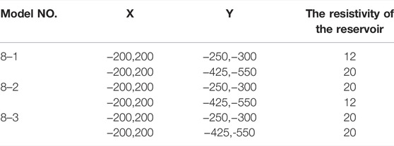
TABLE 9. The model parameters of various vertical distribution combination models of hydrate reservoirs that need to be compared in this group.

In this group of models, the DCR array arrangement of Inline dipole-dipole is used, the electrode spacing a is 25 m, the isolation coefficient n is 8, and the towed height is 30 m. The length of each reservoir is in combination models 400m, and the thickness of the shallower and the deeper reservoir is 50 and 125 m, respectively. The buried depth at the top of the shallower and the deeper reservoir is 100 and 275 m, respectively. The resistivity of marine sediments is 5 Ω·m, and the resistivity of seawater is 0.33 Ω·m. The length of the survey line is 5,000 m. The resistivity of the shallower and the deeper reservoir is the alternating combinations of 12 Ω·m and 20 Ω·m.

3.8.2 Results

The resistivity inversion and hydrate saturation estimation of various dip models of hydrate reservoir (Model 8–1, 8-2, and 8–3) are shown in Figure 11D-I, respectively. The high resistivity range and the high saturation range obtained by the resistivity inversion are basically consistent with the reservoir range in the synthetic model.

FIGURE 11

FIGURE 11. Resistivity inversion and hydrate saturation estimation of various vertical distribution combination models of hydrate reservoir. (A)–(C): the schematic diagram of Model 8–1, 8-2, and 8-3 respectively, light blue indicates seawater, light yellow indicates marine sediments, gray block indicates hydrate reservoirs, dotted line indicates the track of the towed DCR array arrangement; (D), (F) and (H): the inversion resistivity of Model 8–1, 8-2, and 8-3 respectively; (E), (G) and (I): the hydrate saturation estimation of Model 8–1, 8-2, and 8-3 respectively (J): the inversion iteration convergence of Model 8–1(green), 8–2(blue) and 8–3 (red) respectively (K)–(M): the resistivity profile with depth at the center x position of hydrate reservoir of Model 8–1(green), 8–2(blue) and 8–3 (red), respectively.

The depth of the resistivity area basically corresponds to the depth range of the hydrate reservoir. However, there are still differences in the inversion results of these different models. The distribution inversion of the reservoir in Model 8-3 is the best among them. The inversion effect of Model 8-1 is better than that of Model 8–2.

The inversion iteration convergence of the models (Model 8–1, 8-2, and 8–3) are shown in Figure 11J, respectively. The RMS fitting errors of all model calculation results have met the convergence requirements. The fitting iterative in Model 8-2 is not as good as in other models.

We have extracted the resistivity curve of the central position of the hydrate reservoir with depth on the inversion resistivity imaging map, so as to intuitively see the variation of gas hydrate resistivity with depth (Figure 11K-M). The resistivity of hydrate reservoir (12 and 18 Ω·m) in the resistivity inversion results, the anomalies of gas hydrates are reflected with different accuracy.

3.8.3 Discussion

From the comparison between the inversion and the truth resistivity, it can be seen that this method can distinguish between vertically interrupted reservoirs. All reservoirs have a highly resistive resistivity response when the reservoirs have a certain vertically spacing and different resistivity values, which shows that this method has a good ability to distinguish high saturation area from low saturation area.

In the case of the same saturation of shallow and deep reservoirs, the inversion saturation of the shallow reservoir is higher than that of the deep reservoir. If the resistivity of the shallow and deep reservoirs is not consistent, the imaging results can distinguish the presence of upper and lower layers of hydrate on the seafloor, but the saturation and lower boundary may have some bias.

4 Conclusion

(1) After comparing the resistivity imaging results by considering different aspects of the model inversion close to the actual situation, we have found that all these parameters have an impact on reservoir imaging: (a) the DCR array arrangement of the instruments; (b) the towed height of the array arrangement away from the seafloor; (c) the buried depth at the top of the reservoir; (d) the length of gas hydrate reservoir; (e) the thickness of gas hydrate reservoir; (f) the dip of gas hydrate reservoir; (g) the horizontal resolution; (h) the vertical resolution. In practical exploration, we should try to choose more favorable parameters to improve the imaging effect.

(2) The observation of actual resistivity values may be influenced by many factors, so it is not easy to directly evaluate the distribution characteristics of hydrate through resistivity alone. We have proposed to analyze the imaging results using a corrected hydrate saturation equation, which can further improve the ability to evaluate hydrate identification.

(3) After comparing various DCR array arrangements, we have found that a dipole-dipole array arrangement is best suited for identifying the layered structure of hydrate deposits on the seafloor in practical survey operations.

(4) The smaller the distance between the array and the seafloor, the better the exploration effect. Therefore, the towing device should be placed as close to the seafloor as possible in the actual exploration.

Data availability statement

The original contributions presented in the study are included in the article/supplementary material, further inquiries can be directed to the corresponding authors.

Author contributions

NQ: Conceptualization, Data interpretation, Writing, Funding acquisition. QF: Data interpretation, Writing, LY: Data interpretation, Writing, YC: Supervision, Data interpretation, ZS: Supervision, Data interpretation, Funding acquisition. BD: Writing, Funding acquisition.

Funding

This study was funded by Key Special Project for Introduced Talents Team of Southern Marine Science and Engineering Guangdong Laboratory (GML2019ZD0104, 2019BT02H594), Guangdong Basic and Applied Basic Research Foundation (Natural Science Foundation of Guangdong Province) (2021A1515011526), Key Laboratory of Geophysical Electromagnetic Probing Technologies of Ministry of Natural Resources (KLGEPT202001), and Hainan Key Laboratory of Marine Geological Resources and Environment (HNHYDZZYHJKF010).

Conflict of Interest

The authors declare that the research was conducted in the absence of any commercial or financial relationships that could be construed as a potential conflict of interest.

Publisher’s Note

All claims expressed in this article are solely those of the authors and do not necessarily represent those of their affiliated organizations, or those of the publisher, the editors and the reviewers. Any product that may be evaluated in this article, or claim that may be made by its manufacturer, is not guaranteed or endorsed by the publisher.

References

Andreassen, K., Hart, P. E., and Mackay, M. (1997). Amplitude versus Offset Modeling of the Bottom Simulating Reflection Associated with Submarine Gas Hydrates. Mar. Geol. 137, 25–40. doi:10.1016/S0025-3227(96)00076-X

CrossRef Full Text | Google Scholar

Archie, G. E. (1942). The Electrical Resistivity Log as an Aid in Determining Some Reservoir Characteristics. Trans. Am. Inst. Min. Metallurgical Eng. 146, 54–62. doi:10.2118/942054-G

CrossRef Full Text | Google Scholar

Attias, E., Amalokwu, K., Watts, M., Falcon-Suarez, I. H., North, L., Hu, G. W., et al. (2020). Gas Hydrate Quantification at a Pockmark Offshore Norway from Joint Effective Medium Modelling of Resistivity and Seismic Velocity. Mar. Petroleum Geol. 113, 104151. doi:10.1016/j.marpetgeo.2019.104151

CrossRef Full Text | Google Scholar

Becker, K., Davis, E. E., Heesemann, M., Collins, J. A., and Mcguire, J. J. (2020). A Long-Term Geothermal Observatory across Subseafloor Gas Hydrates, IODP Hole U1364A, Cascadia Accretionary Prism. Front. Earth Sci. (Lausanne). 8. doi:10.3389/feart.2020.568566

CrossRef Full Text | Google Scholar

Candansayar, M. E. (2008). Two-dimensional Inversion of Magnetotelluric Data with Consecutive Use of Conjugate Gradient and Least-Squares Solution with Singular Value Decomposition Algorithms. Geophys. Prospect. 56, 141. doi:10.1111/j.1365-2478.2007.00668.x

CrossRef Full Text | Google Scholar

Collett, T. (2013). A Review of Well-Log Analysis Techniques Used to Assess Gas-Hydrate-Bearing Reservoirs, 189–210. 9780875909820.

CrossRef Full Text | Google Scholar

Collett, T. S., and Kuuskraa, V. A. (1998). Hydrates Contain Vast Store of World Gas Resources. Oil Gas J. 96, 90–95.

Google Scholar

Collett, T. S., and Ladd, J. (2000). “19. Detection of Gas Hydrate with Downhole Logs and Assessment of Gas Hydrate Concentrations (Saturations) and Gas Volumes on the Blake Ridge with Electrically Resistivity Log Data,” in Proceedings of the Ocean Drilling Program, Scientific Results, 164. TX, USA: Texas A&M university, college station.

Google Scholar

Cook, A. E., Paganoni, M., Clennell, M. B., Mcnamara, D. D., Nole, M., Wang, X., et al. (2020). Physical Properties and Gas Hydrate at a Near-Seafloor Thrust Fault, Hikurangi Margin, New Zealand. Geophys. Res. Lett. 47. doi:10.1029/2020gl088474

CrossRef Full Text | Google Scholar

Duan, S., Hoelz, S., Dannowski, A., Schwalenberg, K., and Jegen, M. (2021). Study on Gas Hydrate Targets in the Danube Paleo-Delta with a Dual Polarization Controlled-Source Electromagnetic System. Mar. Petroleum Geol. 134, 105330. doi:10.1016/j.marpetgeo.2021.105330

CrossRef Full Text | Google Scholar

Gorman, A. R., and Senger, K. (2010). Defining the Updip Extent of the Gas Hydrate Stability Zone on Continental Margins with Low Geothermal Gradients. J. Geophys. Res. 115, B07105. doi:10.1029/2009jb006680

CrossRef Full Text | Google Scholar

Gundogdu, N. Y., and Candansayar, M. E. (2018). Three-dimensional Regularized Inversion of DC Resistivity Data with Different Stabilizing Functionals. Geophysics 83, E399–E407. doi:10.1190/Geo2017-0558.1

CrossRef Full Text | Google Scholar

Guo, X., Nian, T., Zhao, W., Gu, Z., Liu, C., Liu, X., et al. (2021). Centrifuge Experiment on the Penetration Test for Evaluating Undrained Strength of Deep-Sea Surface Soils. Int. J. Min. Sci. Technol. 32, 363–373. doi:10.1016/j.ijmst.2021.12.005

CrossRef Full Text | Google Scholar

Harinarayana, T., Hardage, B., and Orange, A. (2012). Controlled-source Marine Electromagnetic 2-D Modeling Gas Hydrate Studies. Mar. Geophys. Res. 33, 239–250. doi:10.1007/s11001-012-9159-z

CrossRef Full Text | Google Scholar

Haroon, A., Swidinsky, A., Hoelz, S., Jegen, M., and Tezkan, B. (2020). Step-on versus Step-Off Signals in Time-Domain Controlled Source Electromagnetic Methods Using a Grounded Electric Dipole. Geophys. Prospect. 68, 2825–2844. doi:10.1111/1365-2478.13016

CrossRef Full Text | Google Scholar

Hyndman, R. D., and Spence, G. D. (1992). A Seismic Study of Methane Hydrate Marine Bottom Simulating Reflectors. J. Geophys. Res. 97, 6683. doi:10.1029/92jb00234

CrossRef Full Text | Google Scholar

Jackson, P. D., Taylorsmith, D., and Stanford, P. N. (1978). Resistivity-Porosity-Particle Shape Relationships for Marine Sands. Geophysics 43, 1250–1268. doi:10.1190/1.1440891

CrossRef Full Text | Google Scholar

Kars, M., Greve, A., and Zerbst, L. (2021). Authigenic Greigite as an Indicator of Methane Diffusion in Gas Hydrate-Bearing Sediments of the Hikurangi Margin, New Zealand. Front. Earth Sci. (Lausanne). 9. doi:10.3389/feart.2021.603363

CrossRef Full Text | Google Scholar

Key, K. (2012). Marine Electromagnetic Studies of Seafloor Resources and Tectonics. Surv. Geophys. 33, 135–167. doi:10.1007/s10712-011-9139-x

CrossRef Full Text | Google Scholar

Kvenvolden, K. A. (2000). “Gas Hydrate and Humans,” in Gas Hydrates: Challenges for the Future. Editors G. D. Holder, and P. R. Bishnoi, 17–22. doi:10.1111/j.1749-6632.2000.tb06755.x

CrossRef Full Text | Google Scholar

Lee, M.W., and Collett, T.S. (2006). A method of shaly sand correction for estimating gas hydrate saturations using downhole electrical resistivity log data. Reston, VA: U.S. Geological Survey Scientific Investigations Report 2006-5121, 10.

CrossRef Full Text | Google Scholar

Li, X.-S., Xu, C.-G., Zhang, Y., Ruan, X.-K., Li, G., Wang, Y., et al. (2016). Investigation into Gas Production from Natural Gas Hydrate: A Review. Appl. Energy 172, 286–322. doi:10.1016/j.apenergy.2016.03.101

CrossRef Full Text | Google Scholar

Liu, J., Zhang, J., Ma, F., Wang, M., and Sun, Y. (2017). Estimation of Seismic Velocities and Gas Hydrate Concentrations: a Case Study from the Shenhu Area, Northern South China Sea. Mar. Petroleum Geol. 88, 225–234. doi:10.1016/j.marpetgeo.2017.08.014

CrossRef Full Text | Google Scholar

Liu, P., Huang, H., Hu, L., Mao, S., Tian, Z., Shen, Y., et al. (2022). Hydrate Attenuation Characteristics Based on the Patchy-Saturation Model. Front. Earth Sci. (Lausanne). 10. doi:10.3389/feart.2022.831405

CrossRef Full Text | Google Scholar

Liu, T., Liu, X., and Zhu, T. (2020). Joint Analysis of P-Wave Velocity and Resistivity for Morphology Identification and Quantification of Gas Hydrate. Mar. Petroleum Geol. 112, 104036. doi:10.1016/j.marpetgeo.2019.104036

CrossRef Full Text | Google Scholar

Merle, S. G., Embley, R. W., Johnson, H. P., Lau, T.-K., Phrampus, B. J., Raineault, N. A., et al. (2021). Distribution of Methane Plumes on Cascadia Margin and Implications for the Landward Limit of Methane Hydrate Stability. Front. Earth Sci. (Lausanne). 9. doi:10.3389/feart.2021.531714

CrossRef Full Text | Google Scholar

Oldenburg, D. W., and Li, Y. G. (1994). Inversion of Induced Polarization Data. Geophysics 59, 1327–1341. doi:10.1190/1.1443692

CrossRef Full Text | Google Scholar

Pearson, C. F., Halleck, P. M., Mcguire, P. L., Hermes, R., and Mathews, M. (1983). Natural-Gas Hydrate Deposits - a Review of Insitu Properties. J. Phys. Chem. 87, 4180–4185. doi:10.1021/J100244a041

CrossRef Full Text | Google Scholar

Schwalenberg, K., Gehrmann, R. a. S., Bialas, J., and Rippe, D. (2020). Analysis of Marine Controlled Source Electromagnetic Data for the Assessment of Gas Hydrates in the Danube Deep-Sea Fan, Black Sea. Mar. Petroleum Geol. 122, 104650. doi:10.1016/j.marpetgeo.2020.104650

CrossRef Full Text | Google Scholar

Schwalenberg, K., Haeckel, M., Poort, J., and Jegen, M. (2010a). Evaluation of Gas Hydrate Deposits in an Active Seep Area Using Marine Controlled Source Electromagnetics: Results from Opouawe Bank, Hikurangi Margin, New Zealand. Mar. Geol. 272, 79–88. doi:10.1016/j.margeo.2009.07.006

CrossRef Full Text | Google Scholar

Schwalenberg, K., Wood, W., Pecher, I., Hamdan, L., Henrys, S., Jegen, M., et al. (2010b). Preliminary Interpretation of Electromagnetic, Heat Flow, Seismic, and Geochemical Data for Gas Hydrate Distribution across the Porangahau Ridge, New Zealand. Mar. Geol. 272, 89–98. doi:10.1016/j.margeo.2009.10.024

CrossRef Full Text | Google Scholar

Sloan, E. D., and Koh, C. A. (2007). Clathrate Hydrates of Natural Gases. Boca Raton, FL: CRC Press.0429129149

Google Scholar

Wang, W., Ba, J., Carcione, J. M., Liu, X., and Zhang, L. (2021). Wave Properties of Gas-Hydrate Bearing Sediments Based on Poroelasticity. Front. Earth Sci. (Lausanne). 9. doi:10.3389/feart.2021.640424

CrossRef Full Text | Google Scholar

Wang, X. J., Wu, S. G., and Liu, X. W. (2006). Factors Affecting the Estimation of Gas Hydrate and Free Gas Saturation. Chin. J. Geophys. 49, 441–449. doi:10.1002/cjg2.853

CrossRef Full Text | Google Scholar

Weitemeyer, K. A., Constable, S., and Trehu, A. M. (2011). A Marine Electromagnetic Survey to Detect Gas Hydrate at Hydrate Ridge, Oregon. Geophys. J. Int. 187, 45–62. doi:10.1111/j.1365-246X.2011.05105.x

CrossRef Full Text | Google Scholar

Xu, W., and Ruppel, C. (1999). Predicting the Occurrence, Distribution, and Evolution of Methane Gas Hydrate in Porous Marine Sediments. J. Geophys. Res. 104, 5081–5095. doi:10.1029/1998jb900092

CrossRef Full Text | Google Scholar

Yao, H., Panieri, G., Lehmann, M. F., Himmler, T., and Niemann, H. (2021). Biomarker and Isotopic Composition of Seep Carbonates Record Environmental Conditions in Two Arctic Methane Seeps. Front. Earth Sci. (Lausanne). 8. doi:10.3389/feart.2020.570742

CrossRef Full Text | Google Scholar

Yu, G., Jin, H., and Kong, Q. (2022). Study on Hydrate Risk in the Water Drainage Pipeline for Offshore Natural Gas Hydrate Pilot Production. Front. Earth Sci. (Lausanne). 9. doi:10.3389/feart.2021.816873

CrossRef Full Text | Google Scholar

Zhang, Q., Yang, Z., He, T., Lu, H., and Zhang, Y. (2021). Growth Pattern of Dispersed Methane Hydrates in Brine-Saturated Unconsolidated Sediments via Joint Velocity and Resistivity Analysis. J. Nat. Gas Sci. Eng. 96, 104279. doi:10.1016/j.jngse.2021.104279

CrossRef Full Text | Google Scholar

Zhang, X., Sun, Z., Wang, L., Zhang, X., Zhai, B., Xu, C., et al. (2020). Distribution and Discharge of Dissolved Methane in the Middle Okinawa Trough, East China Sea. Front. Earth Sci. (Lausanne). 8. doi:10.3389/feart.2020.00333

CrossRef Full Text | Google Scholar