Sensitivity of Tropical Cyclone Intensity Variability to Different Stochastic Parameterization Methods

Proper representations of stochastic processes in tropical cyclone (TC) models are critical for capturing TC intensity variability in real-time applications. In this study, three different stochastic parameterization methods, namely, random initial conditions, random parameters, and random forcing, are used to examine TC intensity variation and uncertainties. It is shown that random forcing produces the largest variability of TC intensity at the maximum intensity equilibrium and the fastest intensity error growth during TC rapid intensification using a fidelity-reduced dynamical model and a cloud-resolving model (CM1). In contrast, the random initial condition tends to be more effective during the early stage of TC development but becomes less significant at the mature stage. For the random parameter method, it is found that this approach depends sensitively on how the model parameters are randomized. Specifically, randomizing model parameters at the initial time appears to produce much larger effects on TC intensity variability and error growth compared to randomizing model parameters every model time step, regardless of how large the random noise amplitude is. These results highlight the importance of choosing a random representation scheme to capture proper TC intensity variability in practical applications.

1 Introduction

The application of stochastic physics parameterizations to weather and climate models is a rapidly advancing and important topic in current modeling systems (Palmer, 2001; Christensen et al., 2015; Dorrestijn et al., 2015). Palmer (2012) argued from the theoretical and practical bases that all comprehensive weather and climate models, no matter how complex they are, should be stochastic in nature. From this perspective, although the governing equations are formally deterministic, the best predictions should be based on models that could capture the uncertainty of the atmosphere, whether for climate on long time scales or weather on time scales of days to weeks. Developing practical tools for estimating such uncertainty of model forecasts would require the knowledge of random error effects, which then allows us to investigate the relative impacts of different types of uncertainties in models.

In general, TC intensity forecast errors in any numerical model are caused by several factors, including model errors, vortex initial uncertainties, global boundary guidance errors, random environmental forcings, and/or the intrinsic nature of TC intensity variability (Gopalakrishnan et al., 2011; Tallapragada et al., 2012; Kieu et al., 2018; Halperin and Torn, 2018; Trabing and Bell, 2020; Kieu et al., 2021, NKF). While these factors are technically non-separable in practice due to the nonlinear nature of TC dynamics and thermodynamics, it is possible to examine their relative roles under some specific conditions. For example, real-time verification of TC intensity forecast shows that model errors tend to be more important at a longer lead time compared to vortex initial condition errors (Du et al., 2013; Kieu et al., 2021). Likewise, uncertainties in global lateral boundary conditions could result in a wrong track forecast, which can lead to large intensity errors for incorrect landfalling storms or TCs under rapidly changing environments, even in perfect regional models with perfect initial conditions as discussed in Kieu et al. (2021).

Among those sources of intensity errors, the impacts of different random types on TC intensity variability appear to be the least examined. Even under the most idealized conditions with no other sources of model or initial condition errors, the atmospheric random fluctuation always exists and introduces uncontrollable uncertainties into TC development. While these random fluctuations are often small and probably less important than other types, such as model or initial condition errors, the nonlinearity of TC dynamics could amplify random fluctuations during TC development and eventually lead to noticeable variability in TC intensity that is currently not fully understood.

Despite such an inherent random nature of the atmosphere, examining how it affects TC intensity, especially the relative importance of different stochastic representations during TC intensification, is still an open question due to how random noise is parameterized in TC models. Using a low-order TC model (Nguyen et al., 2020, hereinafter NKF), recently examined the effects of random noise in terms of the Wiener process at the maximum intensity equilibrium. By analyzing the invariant intensity distribution at the mature stage, they showed that the stochastic forcing associated with tangential wind and warm-core anomaly has the largest contribution to TC intensity variability. This theoretical result is consistent with previous modeling studies, which captured strong sensitivity of TC intensity to vortex initialization schemes and warm-core retrieval in TC models (Kurihara et al., 1995; Liu et al., 2000; Van Nguyen and Chen, 2011; Rappin et al., 2013; Zou and Tian, 2018). How the effects of stochastic forcing are compared to those caused by random parameters or the vortex initial condition have not been addressed.

In this study, we wish to examine how different methods of representing atmospheric random noise will affect the variability of TC intensity and the intensity error growth during TC rapid intensification. Understanding the relative roles of stochastic parameterization approaches in TC intensity variability will help quantify an intensity error limit that one can achieve with numerical models in the future. Likewise, examining the error growth during the intensifying stage will help evaluate how the accuracy of the TC intensity forecast evolves during TC development for operational applications. For this purpose, we will use both a fidelity-reduced TC model (Kieu, 2015; Kieu and Wang, 2017, hereinafter KW17) and the cloud-resolving (CM1 Bryan and Fritsch, (2002)) model to study the effectiveness of different stochastic representation methods in capturing TC intensity fluctuations.

The structure of the article is organized as follows: Section 2.1 presents a brief introduction of the TC-scale dynamical model, its extension for a stochastic system, and different types of random representations. Section 2.2 discusses the application of stochastic parameterization for the CM1 model. A detailed algorithm to calculate the error growth during the rapid intensification is provided in Section 2.3. The results from the fidelity-reduced model are presented in Section 3, while error saturation at the mature stage and error growth for the CM1 model are discussed in Section 4. Finally, some concluding remarks are given in Section 5.

2 Methodology

2.1 Fidelity-Reduced TC Model

Given the complex nature of TC dynamics, a complete investigation of different stochastic mechanisms in full-physics TC models is generally not feasible. This is because full-physics models are highly nonlinear with various parameterization schemes that not only require a large computational resource to conduct stochastic simulations but also introduce insurmountable difficulty in analyzing nonlinear interactions among different physical components.

As a first step to examine the effects of different stochastic parameterizations on TC intensity, a simple model for TC development is needed. Among several existing low-order TC models, the TC-scale model proposed by Kieu (2015) and modified further by KW17 (hereinafter referred to as the modified TC-scale dynamics, or MSD, model) is of specific interest. Using TC scales as dynamical variables in the axisymmetric framework, the scale analyses of the governing equation can be reduced to a set of ordinary differential equations that contain only a few TC basic scales, including the maximum tangential wind (v), the maximum radial wind at the surface (u), and the warm anomaly in the TC central region (b). With the wind-induced surface heat exchange feedback closure, these non-dimensional scale equations are given as follows:

$\dot{u}=p{v}^2-\left(p+1\right)b-C_{d}u|v|,(1)$

$\dot{v}=-uv-C_{d}v|v|,(2)$

$\dot{b}=bu+su+T_s|v|-rb.(3)$

This MSD model includes several parameters (p, s, r, C _d , T _s ) that characterize the TC dynamics, where p is a constant proportional to the squared ratio of the depth of the troposphere to the depth of the boundary layer, s denotes the effective tropospheric static stability, r represents the Newtonian cooling, and C _d and T _s are non-dimensional parameters representing the surface drag coefficient and sea surface temperature (SST). Note that, unlike the original MSD system in KW17, for which C _d and T _s are scaled to have a value of 1, we retain their explicit role in this study such that the sensitivity of TC intensity and the error growth to these parameters can be explored.

While the MSD model is simple, it has some properties that are attractive for our investigation of random representations in this study. First, this system is explicitly time-dependent, which is required to examine the evolution of TC intensity and related error growth during TC intensification. Second, the model contains the maximum potential intensity (MPI) limit as its unique stable point in the phase space of (u, v, b), as discussed in KW17. The existence of such a stable point is vital because it allows us to quantify how the variability of TC intensity at the mature stage depends on different random parameterization methods, as discussed in NKF.

While the MSD system could describe both cyclonic and anticyclonic flows as discussed in Kieu and Wang (2018), we will limit our consideration hereinafter to cyclonic TCs in the Northern Hemisphere such that the absolute signs in Eqs 1–3 can be removed. In the next sections, we will describe three different random mechanisms and how to implement them for the MSD system. These mechanisms include 1) random forcing, 2) random initial condition, and 3) random parameters, which are the most commonly used methods in the current numerical weather prediction models.

2.1.1 Random Forcing (RF) Representation

We first examine a type of random representation in which the model forcing is augmented by stochastic processes, often known also as physical stochastic parameterization (Palmer, 2001; Christensen et al., 2015; Dorrestijn et al., 2015). According to this method, random noise is added to prognostic variable tendencies or model states with different spatial and temporal scales (Palmer, 2001; Weisheimer et al., 2011; Zhang et al., 2015; Christensen, 2020). This approach is equivalent to adding random noise to model forcing (NKF, Fan et al., 2021a), which will be hereinafter referred to as the random forcing (RF) method.

Following NKF, we introduce additive driving noise in terms of the Wiener process to the MSD system (1–3) and obtain the following stochastic differential equations:

$d{U}_t=\left(p{V}_t^2-\left(p+1\right)B_t-C_d{U}_t{V}_t\right)dt+{\sigma }_{u}d{W}_t^{\left(u\right)},(4)$

$d{V}_t=\left(-U_t{V}_t-C_d{V}_t{V}_t\right)dt+{\sigma }_{v}d{W}_t^{\left(v\right)},(5)$

$d{B}_t=\left(B_t{U}_t+s{U}_t+T_s{V}_t-r{B}_t\right)dt+{\sigma }_{b}d{W}_t^{\left(b\right)},(6)$

where {W ^(u), W ^(v), W ^(b)} are independent Wiener processes and (σ _u , σ _v , σ _b ) are the corresponding noise amplitude. While parameterizing stochastic forcings by the Wiener process appears to be reasonable, we note that the assumption of stochastic forcings as state-independent noise requires some justification because real stochastic forcings may be functions of atmospheric states instead of having a constant variance. Because our focus here is on the relative roles of different stochastic parameterization methods in TC intensity rather than the physical nature of each forcing term, we will choose this constant-variance stochastic forcing as a protocol for the RF method to compare with the other random methods. More detailed discussion of this assumption can be found in (NKF) Fan et al. (2021b).

With the RF representation in terms of the Wiener process, the numerical solution of Eqs (4–6) can be easily obtained using Monte Carlo simulations. In this study particularly, the Runge–Kutta fourth-order scheme is applied to the deterministic part of Eqs (4–6) with a discretized time-step Δt, identical to that used in NKF. The stochastic part is then added to the model forcing at each time step, using a Gaussian random variable with variance $(\mathrm{\Delta }t){\sigma }_i^2$ for each state variable i ∈ {u, v, b}. Because of the constant variance for the stochastic forcings, this approach is essentially equivalent to the Euler–Maruyama first-order scheme. So long as the time step Δt is sufficiently small, this first-order accuracy suffices for representing the random processes as expected.

2.1.2 Random Parameter (RP) Representation

The second common method for parameterizing stochastic processes in numerical models is to randomize model parameters based on a prior probability distribution of the parameters. A rationale behind this approach is that model parameters cannot be known accurately due to measurement uncertainties, incomplete understanding of physical processes, or the stochastic nature of phase transitions. For example, Zhang et al. (2015) implemented a mechanism that allows random fluctuation in the convective triggering function in an operational ensemble system, which is simply a numerical flag in the convection parameterization of the Hurricane Weather Research and Forecasting (HWRF) model. Similarly, other studies have applied the RP approach to, for example, the boundary parameterization to reflect the unknown variations in the land surface and/or boundary processes (Song et al., 2007; Plant and Craig, 2008; Doblas-Reyes, 2009; Breil and Schädler, 2017). This RP scheme has been shown to improve the model overall ensemble spread, thus capturing better the uncertainties of model physics than deterministic ensembles.

Given these inherent uncertainties of model parameters, we implement a scheme for the MSD model in which three key model parameters, including the tropospheric static stability (s), the sea surface temperature T _s , and the surface drag coefficient (C _d ), are randomized around a given mean value. Generally, such model parameter randomization can be carried out in two different ways. In the first approach, random noise is introduced to model parameters at the beginning of the model integration and kept unchanged during the entire integration (hereinafter referred to as the initial RP approach). In the second approach, random noise is added to model parameters every time step during the integration to reflect the variability of these model parameters with time (hereinafter referred to as the time-varying RP approach).

While both the initial and time-varying RP approaches are practical and can be compared with each other, their mathematical and physical interpretations are quite different and require detailed examinations. For the initial RP approach, the uncertainties in the model parameters enter the system only as measurement errors, which prevent one from determining the model parameters accurately. Thus, model parameters take random values at the initial time but are fixed during the course of the model integration. In contrast, the time-varying RP method accounts for the fact that model parameters are itself a random function of time that must have a statistical distribution. An example of this is the convective triggering function in cumulus parameterization, which determines if deep convective plumes can occur or not (Arakawa and Schubert, 1974; Kain and Fritsch, 1990; Song et al., 2007; Suhas and Zhang, 2014; Zhang et al., 2015). This triggering function often depends on vertical motion, CAPE, or some other ambient variables, so it is inherently a random function of time. In this regard, the outcome from the initial RP and time-varying RP representation could bring different insights into the variability of TC intensity that we wish to explore herein.

To be specific for our implementation in this study, the three model parameters (s, T _s , C _d ) are assumed to be Gaussian random variables with known means and standard deviations. In non-dimensional units, the mean and standard deviation values are $\bar{s}=0.1$ and σ _s = 0.01 for the static stability s, $\bar{T}=1$ and ${\sigma }_{T_s}=0.1$ for SST T _s , and $\bar{C}=1$ and ${\sigma }_{C_d}=0.1$ for the surface drag coefficient C _d . These mean values are based on their observed magnitude in real TC-force wind environment (Kieu, 2015; Zhang, 2010), while the standard deviations are assumed to be 10% of the mean values based on the typical observational errors for TCs (Zhang, 2010; Richter et al., 2021). Because we wish to examine the relative importance of RF and RP approaches, no random noise is added to the model forcings in both the initial and time-varying RP implementations.

2.1.3 Random Initial Condition (RIC) Representation

The last approach to consider stochastic processes is to randomize model initial conditions, which is by far the most common method to account for uncertainties in operational models (Hamill et al., 2011; Aksoy et al., 2013; Aberson et al., 2015; Zhang and Weng, 2015; Tong et al., 2018). Often known as ensemble forecasting, the RIC approach introduces noise with a given probability distribution to reflect the initial condition uncertainties. This probability distribution comes from various pathways such as a prior background covariance matrix (cold-start), ensemble cycling (breeding), or an analysis covariance matrix (data assimilation), which are generally given at all model grid points.

Following the common practice of implementing random initial uncertainties in previous studies, our RIC method adds white noise to the MSD model initial conditions, using a Gaussian distribution with a given variance and zero mean. In the non-dimensional unit, the white noise for the RIC method with the MSD model has a standard deviation of 0.01 for all (u, v, b) components. In full physical dimension, this standard deviation respectively corresponds to $\sim 1m{s}^{-1}$ for wind and $\sim 0.5K$ for temperature, which are reasonable for the random wind and temperature noise in real atmospheric conditions (Zhang, 2010; Zhang et al., 2010). Note that, unlike the RF or time-varying RP method for which the randomness is realized at every time step, the RIC representation introduces random noise only at the initial time, similar to the initial RP method. Therefore, conditioned on the realization of the random initial condition, the MSD model is deterministic at all time for the RIC method.

Given the above approaches to represent stochastic processes in the MSD model, Monte Carlo simulations of 1,000 members are then carried out to examine the variability of TC intensity and the error growth rate for each random representation method. In our range of Monte Carlo experiments, we observe that an ensemble of $>$ 100 realizations is generally sufficient for a stable statistical distribution and significance. Given the cheap computational cost of the MSD model, a fixed number of 1,000 realizations is therefore used for all the RIC, RP, and RF methods in this study such that the ensemble-size sensitivity analyses are not necessary.

2.2 CM1 Model Experiments

While the MSD system could allow detailed examinations of the relative impacts of different random representations due to its efficient computation and low order, real TCs are much more complex, with various nonlinear feedback between different dynamics and thermodynamics components that are not accounted for in the MSD model. In addition, TC dynamics may contain chaotic behaviors at the MPI equilibrium, which can mask the stochastic effects that the MSD model could not capture (Kieu et al., 2018; Keshavamurthy and Kieu, 2021, NKF).

To further evaluate the relative effects of random representations on TC intensity, the cloud model (CM1, Bryan and Fritsch (2002)) is therefore employed in this study. By implementing different random mechanisms in the CM1 model, one can verify what results obtained from the MSD system are valid in a more complete full-physics model and thus applicable to real TCs. For our herein study, the axisymmetric setting of the CM1 model was used such that the results from the CM1 model can be used to verify those obtained from the MSD model under the same axisymmetric framework. Comparing analyses from the low-order MSD model and the full-physics CM1 model can therefore provide more understanding of the impacts of random noise on the variability and the error growth of TC intensity.

Because of the large computational requirement and the numerical stability of the CM1 model, it is noted that our implementation of the RF method for the CM1 model is slightly different from that for the MSD model. Specifically, we apply additive white noise to the momentum and temperature equations with a constant standard deviation of [0.1–0.5]m s ⁻¹ min⁻¹ for wind and [10^–3 − 10^–2]K min⁻¹ for temperature, respectively (Zhang, 2010; Zhang et al., 2010). The constant variance design is to ensure the closest possible resemblance to the RF implementation for the MSD system described in the previous section. It also helps maintain the same order of the finite difference accuracy for the deterministic part, which is based on the Runge–Kutta scheme in the CM1 model. However, no random noise is added to the model moisture state variable due to unknown probability distributions of moist variables/graupel species. Our attempt to add random noise to moist variables did not show any significant difference in terms of model intensity output. However, the noise decreases the stability of the CM1 model and prevents examining a range of noise amplitude dependence. Thus, no random perturbations are applied to the moist equations in all of our CM1 experiments herein.

Regarding the RIC method, our approach for the CM1 model is identical to that for the MSD model. In other words, white noise with a range of standard deviations from 0.01 to 0.1 ms ⁻¹ is added to the CM1 model’s initial conditions. Likewise, the implementation of the RP method for the CM1 model is also identical to that used in the MSD model. Nonetheless, it should be noted that CM1 has many model parameters that can be randomized. For comparison with the MSD model, two specific parameters that are directly relevant to the TC intensity in CM1, including the sea surface temperature (T _s ) and the surface drag (C _d ), are chosen in our RP experiments with the CM1 model. These parameters are assumed to be random variables with a standard derivation of 1 K for T _s and 10^–4 for C _d , respectively. The mean values for these parameters are then varied in the range of [298–305 K] for T _s and [10^–3 − 3 × 10^–3] for C _d such that the dependence of TC intensity variability on different mean values of model parameters can also be studied. Note that tropospheric stratification is a parameter in the MSD model, but it is a diagnostic variable in CM1. Therefore, its random parameterization cannot be implemented in the CM1 model.

Due to the computational limit and a large number of model output, a fixed number of 100 realizations are conducted for each random noise amplitude in the CM1 experiments, regardless of the random representation method. Our ad hoc sensitivity analyses for ensemble members ranging from 100 to 200 show again insignificant differences in terms of statistics when the number of realizations changes. Thus, no ensemble size sensitivity experiment for CM1 will be provided.

2.3 An Error Growth Algorithm

To evaluate the effects of random noise on TC intensity error growth, we follow the approach of Kieu et al. (2018) and introduce small noise along a reference state at different stages of TC development. This type of state-dependent error growth rate mimics the real-time forecast cycles by which the TC intensity forecasts are re-initialized every 6 or 12 h. As TCs evolve, their intensity changes and TC intensity errors may therefore evolve differently, even with the same initial error. Examining how such an intensity error growth rate changes with time will allow forecasters to estimate how the accuracy of their intensity forecast varies during TC development.

In quantifying the dependence of intensity error growth on the stage of TC development, it is important to note that all environmental conditions must be fixed so that such dependence can be well-defined because any change in environmental conditions would cause not only changes in TC intensity along the trajectory but also a shift in the MPI equilibrium, which produces an unexpected intensity error variability. This is a subtle point in studying TC intensity errors, yet it has not been sufficiently emphasized in previous studies that we wish to emphasize again here.

With this approach, our algorithm for computing TC intensity error growth in the MSD model includes the following steps.

1) Select any initial state x ₀ = (u ₀, v ₀, b ₀), where v ₀ > 0 and generate a reference orbit x _f (t) = (u _f (t), v _f (t), b _f (t)) during a given interval t ∈ [0, T], based on the deterministic MSD system (1–3) (see the thick black line in Figure 1A);

2) Choose a given time τ and its corresponding reference state x _f (τ) at the time τ to add a random perturbation vector ξ to x _τ , where ξ = (ξ _u , ξ _v , ξ _b ) are independent Gaussian variables with zero mean and standard deviations {σ _u , σ _v , σ _b }, respectively. This process gives us an initially perturbed state x _f (τ) + ξ at time τ (see the crosses in Figure 1A);

3) Denote the components of the perturbed state at τ as (u′(τ), v′(τ), b′(τ)) ≡ x _f (τ) + ξ; we then choose a lead time Δ and integrate (u′(τ), v′(τ), b′(τ)) from 0 to Δ, using the same MSD model as for the reference integration;

4) For each pair (τ, Δ), repeat steps 2–3 several times (e.g., N = 1,000 times) to generate an ensemble of integration from the initially perturbed state (u′(τ), v′(τ), b′(τ)). Note that different realizations of the Gaussian distribution will give different ξ, even with the same values of mean and standard deviation. Store all of these integrated states and denote their corresponding states at t = τ + Δ as (u _i (τ + Δ), v _i (τ + Δ), b _i (τ + Δ)), i = 1..N (see the triangles in Figure 1B);

5) Compute the root mean square error err (τ, Δ) for the v _i (τ + Δ) component with respect to the reference component v _f (τ + Δ) for each time τ and lead time Δ as follows:

$err\left(\tau ,\mathrm{\Delta }\right)=\sqrt{\frac{1}{N}\sum _{i=1}^N{\left(\frac{v_i\left(\tau +\mathrm{\Delta }\right)-v_f\left(\tau +\mathrm{\Delta }\right)}{\mathrm{\Delta }}\right)}^2},(7)$

which is defined hereafter as the intensity error growth rate corresponding to the lead time Δ at the forecast cycle τ.

6) Repeat steps 1–5 for different values of τ and Δ to obtain the distribution of the error growth rate as a function of (τ, Δ).

FIGURE 1

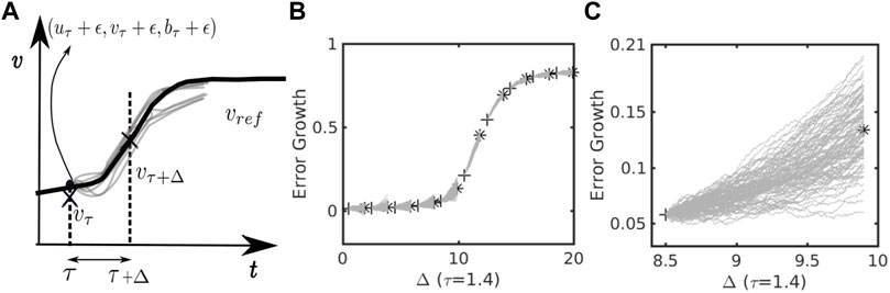
FIGURE 1. A schematic diagram illustrating the algorithm for calculating TC intensity error growth at different stages of TC development for (A) a reference orbit (solid black) and an ensemble of perturbed stages at the beginning time τ and the end of the perturbation integration τ + Δ (crosses); (B) time series for a range of stages starting from τ and ending at τ + Δ for N = 1,000 realization; and (C) a magnified version of (B) for one specific stage. Note that pluses and asterisks in (B,C) show the points on the deterministic orbit at time τ when perturbations are added and at time τ + Δ where the error growth rate is computed, respectively.

By varying τ, the error growth calculation as outlined above can capture the characteristics of TC intensity error at different stages of TC development. Likewise, varying Δ will allow us to examine how TC intensity error growth changes with forecast lead times similar to what is carried out in real-time intensity verification. Note that our definition of the intensity error growth in Eq. 7 is relative to a given reference state v _f (τ + Δ). If one replaces this reference state with the corresponding ensemble mean, Eq. 7 would give us an ensemble spread instead of the absolute intensity errors. As our focus here is on the growth of the absolute error rather than the ensemble mean, definition (7) is therefore adopted here.

Although the same steps are carried out for all three random representation methods, we should mention that different realizations of ξ are added to the initial state only for the RIC method because the MSD system (1)–(3) is deterministic. For the RF method, stochastic forcing varies every time step, so there is no need to randomize the initial state. For the RP method, whether one applies different realizations of the initial perturbation ξ would depend on what RP scheme (i.e., the initial or time-varying) is used, as discussed in the previous section.

3 Fidelity-Reduced Model Results

In this section, we present first the analyses of different random representation methods for TC intensity in the MSD model, using two key measures, including 1) TC intensity variability at the maximum equilibrium and 2) intensity error growth. The first measure provides insights into TC intensity error saturation at long forecast lead times, which plays a key role in estimating TC intensity predictability, as discussed by Kieu and Moon (2016) and Kieu et al. (2018). The second measure focuses on how the characteristics of TC intensity error growth change during TC development, relevant to the reliability of the operational forecast. These two aspects of TC intensity can be thoroughly examined within the low-order MSD model and compose the main results of this section.

3.1 Intensity Variability at the Mature Stage

To have a broad picture of TC intensity in our stochastic MSD model, Figure 2 shows the time series of the v-component in the MSD system as obtained from the Monte Carlo simulations with the RF method. These simulations have the same numerical procedure and settings as in NKF, which are summarized in Table 1. Note that the v component represents the maximum tangential wind near the surface in the TC-scale dynamics. Thus, it can be used as a proxy to examine TC intensity and related variability in all following analyses.

FIGURE 2

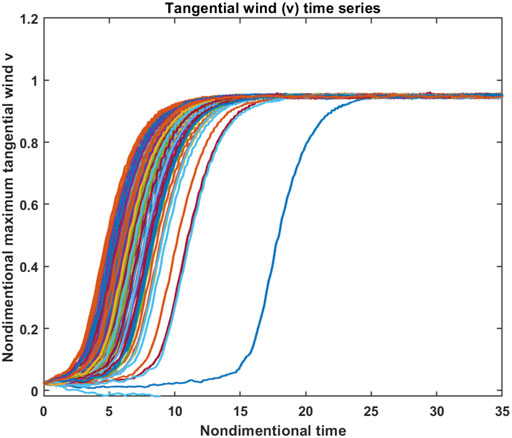
FIGURE 2. Time series of the tangential wind component v as obtained from 1,000 Monte Carlo simulations of the MSD system, using the random forcing representation with noise amplitude σ = 0.01. Model initial condition is set as (−0.01, 0.01, 0.01), and other model parameters are p = 200, s = 0.1, r = 0.25, C _d = 1.0, T _s = 1.0.

TABLE 1

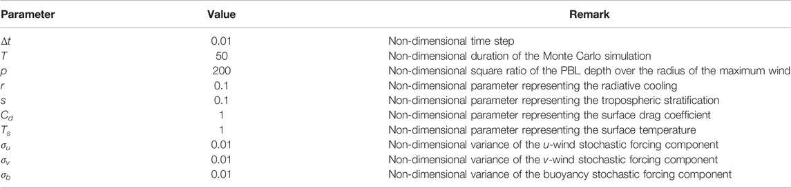
TABLE 1. Configuration of Monte Carlo simulations for the stochastic MSD model (4)–(6). Details of physical interpretations and scaling analyses of these parameters can be found in KW17.

As shown in Figure 2, the Monte Carlo simulations of Eqs 4–6 overall capture expected TC development, with three distinct phases in all realizations, including a pre-condition (genesis) period, rapid intensification, and finally, the maximum intensity equilibrium stage. While the exact onset moment of rapid intensification highly varies among realizations (Fan W.-T. et al. 2021), these three stages are well displayed and reflect the inherent TC development in the MSD model under an idealized environment, even in the presence of random noise. Despite a similar intensification rate among all realizations, the stochastic nature of the MSD model is manifested in Figure 2 as non-smooth fluctuations of TC intensity every time step along any trajectory. So long as the model parameters are fixed, the random forcing affects only fluctuations around the main trajectory but not the averaged state of TC development. As the RF amplitude increases, TC mean state is no longer maintained and the intensification rate or MPI will differ. In this regard, these Monte Carlo simulations confirm not only the main characteristics of TC development but also the stochastic property of the MSD system (4)–(6) with the RF representation as expected.

However, of more interest for our analyses is the variability of TC intensity at the maximum intensity equilibrium due to stochastic forcing, which dictates the limit in our ability to reduce TC intensity forecast errors. To examine how this variability depends on the amplitude of each RF in Eqs 4–6, Figure 3 shows the standard deviation of v (denoted hereinafter as Γ) as a function of (σ _u , σ _v , σ _b ) during the equilibrium stage (i.e., t = 25–50 in Figure 2). Consistent with the results of Nguyen et al. (2020) (Figure 4), TC intensity fluctuations increase almost linearly with σ _u and σ _v , so long as these RF amplitudes are sufficiently small (<0.05 in non-dimensional unit). Such an asymptotically linear increase of Γ for the small noise can be proven rigorously based on the stationary distribution, as shown in NKF.

FIGURE 3

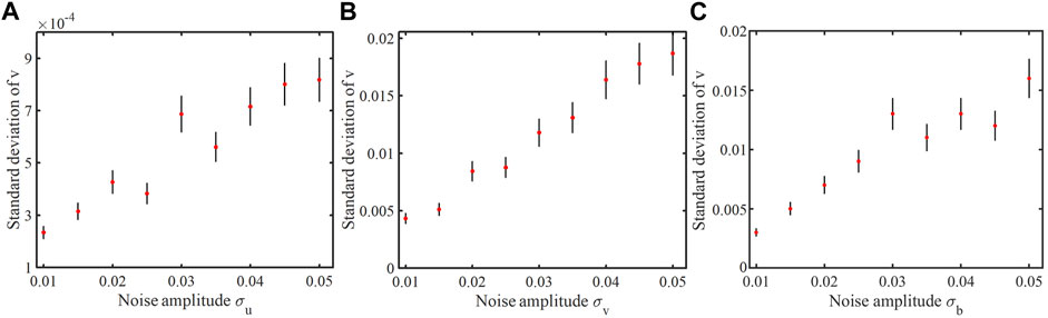
FIGURE 3. The standard deviation of the v component for the RF representation method as a function of the stochastic forcing standard deviation added to (A) the u forcing, (B) the v forcing, (C) and the b forcing in the MSD system.

FIGURE 4

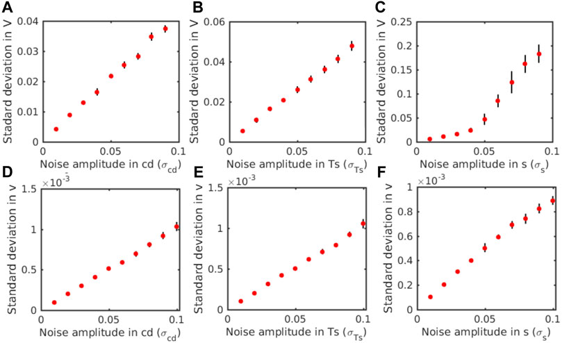
FIGURE 4. Similar to Figure 3 but for the RP representation as a function of the random standard deviation for (A–C) initial RP and (D–F) time-varying RP method.

For the stochastic forcing component σ _b , we note that Γ differs somewhat from a linear function because it is possible that TC intensity deviates far away from the equilibrium when σ _b is sufficiently large, and the underlying stability assumption for the MSD system is thus no longer valid. Consistent with the finding in NKF, we also notice that the stochastic forcing for tangential wind or warm-core anomaly has the most impact on overall TC intensity variability (Figures 3B,C), which produces intensity fluctuation one order of magnitude larger than that caused by the radial wind stochastic forcing (Figure 3A).

Relative to the RF method, Figure 4 shows a similar dependence of Γ on each model parameter at the MPI equilibrium obtained from the initial and time-varying RP methods. Overall, intensity fluctuation increases with the magnitude of the parameter variance for both the RP implementations, similar to that with the RF method. However, one notices a fundamental difference between the RP and RF methods in terms of the magnitude of Γ. Particularly in the initial RP method (Figures 4A–C), Γ is of the same order of magnitude as in the RF method. In contrast, the time-varying RP method (Figures 4E,F) captures almost one order of magnitude smaller regardless of model parameters. This is a noteworthy point because it suggests that the randomness of the model parameters during TC development plays a less important role in TC intensity variability than the initial uncertainty in these model parameters. From a practical standpoint, this non-trivial result implies that our efforts in improving model parameters at the initial time will have more effects on TC intensity variability than randomly sampling model parameters during the course of model integration.

From the mathematical standpoint, such different behaviors of intensity variation between the initial and the time-varying RP approaches can be understood if one analyzes the intensity probability distribution at the equilibrium as in NKF. Indeed, sensitivity analyses of the intensity variance for the initial RP method at the MPI limit (Supplementary Appendix S1) show that the tropospheric static stability parameter s plays a smaller role in the overall variability of TC intensity when s is small. As s becomes sufficiently large ( $>$ 0.04), the MSD system becomes bifurcated Kieu and Wang (2018) and the deviation around the MPI equilibrium becomes much larger, thus resulting in larger Γ as seen in Figure 4C. On the contrary, the SST and surface drag coefficient parameters do not possess any bifurcation point. Therefore, Γ increases almost linearly with the random noise amplitude for the initial RP representation ¹ . This result highlights the critical role of the tropospheric static stability in determining TC intensity variability compared to C _d or SST (KW17, Kieu et al., 2021).

Unlike the initial RP method, for which the MPI may settle down to different equilibria for different parameters, the time-varying RP method has a much more intriguing behavior. Herein, we study an important property of a linear stochastic system with time-varying random parameters, for which the fluctuation of the system around its stable point approaches zero as the numerical time step becomes finer (see Supplementary Appendix S2). This counter-intuitive behavior in the presence of pure random parameters is because a finer time step prevents the model state from deviating too far from its equilibrium at each iteration, leading to an overall smaller fluctuation with time when the time step decreases. While the MSD system is far from linear, the MSD system, under random forcing, captures smaller Γ for a smaller time step in our series of experiments, much like a linear system (not shown). This particular property of the time-varying RP indicates the subtle dependence of TC intensity variability on the way one implements the RP representation in TC models, as shown in Figure 4.

Although the initial and time-varying RP methods result in a different response of TC intensity to random parameters, it is of interest to note that Γ is somewhat the same among the three model parameters for each method in terms of magnitude. This indicates that the random fluctuation of each parameter could equally induce TC intensity variability that one has to consider. Of course, these relative roles among these parameters, as shown in Figure 4, are very specific to the MSD model. Therefore, it is necessary to further verify these properties in full physics models, as shown in Section 4.

Unlike the RF or RP approach, for which the stochasticity can take place at every time step, the RIC method is different due to the deterministic nature of the underlying model. We note again that the MSD model contains a single stable point that corresponds to the MPI equilibrium, as shown in KW17. Thus, regardless of initial conditions, all trajectories will eventually converge to a single MPI point after a sufficiently long time. In the absence of stochastic forcing or random parameters, the intensity variability at the MPI equilibrium in the MSD model must therefore approach zero irrespective of the initial random components, as confirmed in Figure 5. Apparently, this deterministic characteristic of the MSD system prevents it from modeling TC intensity variability at the MPI limit unless stochastic forcing or random parameters are used.

FIGURE 5

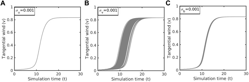
FIGURE 5. Time series of tangential wind v for a fixed noise amplitude σ _u,v,b = 0.001 that is added to initial condition (A) u ₀, (B) v ₀, (C) b ₀, respectively, where the initial condition (u ₀, v ₀, b ₀) = (−0.01, 0.01, 0.01), and other model parameters are p = 200, s = 0.1, r = 0.25, C _d = 1.0, T _s = 1.0.

We wish to mention at this point that real TC dynamics is far more complex than a single stable point at the equilibrium captured by the MSD system, as shown in Figure 5. As discussed in previous studies (Hakim, 2011; Brown and Hakim, 2013; Kieu and Moon, 2016), long simulations of any full-physics TC model always display a quasi-stationary equilibrium instead of a stable fixed point as in the MSD system or the theoretical MPI framework. Such intensity fluctuation at the MPI limit in real TC models could be attributed to several factors, such as process noises, truncation errors, or the existence of low-dimensional chaotic dynamics, none of which is captured by the MSD system. To better compare the relative effects of the RIC, RF, and RP methods in representing random effects on TC intensity, one must ultimately employ full physics models. For the MSD system, we could at least conclude that the RF method produces the largest impact on TC intensity variability at the long lead times, followed by the initial RP method. To what extent this can be realized in full-physics CM1 models will be presented in Section 4.

3.2 Error Growth During RI

Along with the variability of TC intensity at the equilibrium, it is necessary to examine also how intensity fluctuation varies during TC development. In this regard, Figure 6 shows the TC intensity error growth rate err (τ, Δ) as a function of forecast lead time τ for the RF method. Recall that the error growth rate is computed along a reference trajectory with a prescribed lead time Δ. Thus, err (τ, Δ) depends on both the integration time (τ) and the lead time Δ, as discussed in Section 2.3.

FIGURE 6

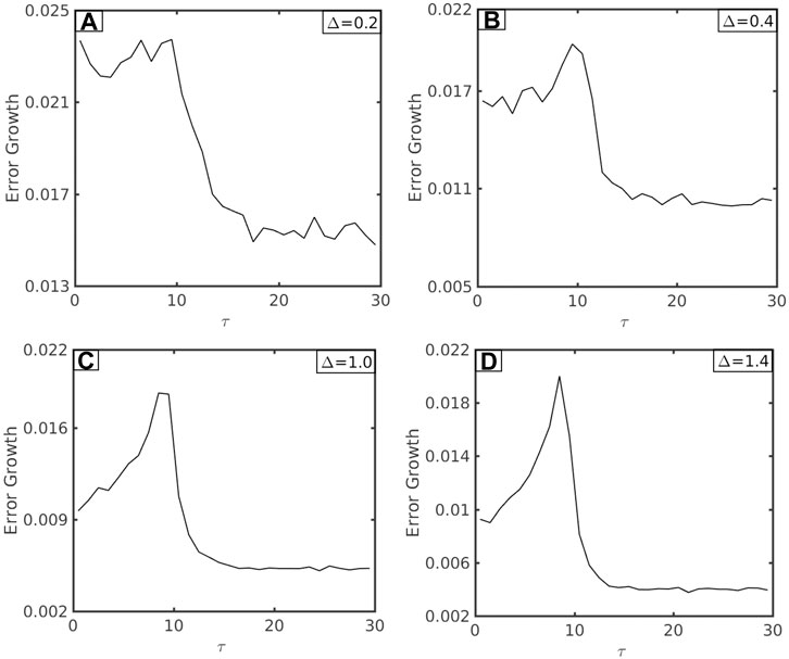
FIGURE 6. The intensity error growth rate err (τ, Δ) for different values of the forecast lead time Δ and the stage of development (τ) as obtained from the RF method, using the same set of model parameters as in Figure 3 with σ _u = σ _v = σ _b = 0.01. For (A) Δ = 0.2, (B) Δ = 0.4, (C) Δ = 1.0, and (D) Δ = 1.4. Here, fixed perturbation amplitude ϵ = 0.001 and N = 1,000 realizations are used for all error growth integration.

Regardless of the forecast lead time Δ, one can see in Figure 6 a very specific pattern of err (τ, Δ), with the most rapid growth during the pre-conditioning stage, followed by a quick decrease during the intensification period and eventually approaching a constant growth rate at the MPI equilibrium. err (τ, Δ) as maximum prior to rapid intensification reflects the fact that the onset moment of TC rapid intensification highly varies among different realizations in the MSD system (cf. Figure 2; see also Fan et al. (2021b) for a rigorous treatment), thus resulting in large intensity errors. As the vortex enters its intensification period, TC dynamics becomes more consistent among all realizations, which explains the decrease in error growth. In contrast, the growth rate is minimum when the TC vortex reaches its equilibrium stage because this equilibrium is highly stable and resilient to random fluctuation (Kieu, 2015, NKF). As a result, err (τ, Δ) subsides and levels off for τ > 16. These behaviors of the intensity error growth rate accord with a previous study using a full-physics model (Kieu et al., 2018) and highlight the unique properties of TC intensity errors.

Of further significance is that the overall error growth characteristics of err (τ, Δ) appear to be less sensitive to the forecast lead time Δ, so long as Δ is not too large. However, note for the RF method that err (τ, Δ) is smaller for a longer lead time Δ, as shown in Figure 6. This smaller error growth rate for a longer lead time is because TC intensity is bounded by the maximum equilibrium. Therefore, a long forecast lead time Δ must eventually result in a reduced error growth rate, as seen from Eq. 7 as TC intensity approaches the MPI limit Kieu et al. (2018), consistent with what was shown in Figure 6.

For the RIC method, a very similar behavior of err (τ, Δ) is captured, with the maximum rate during the pre-conditioning period, followed by a decrease during rapid intensification and a stable value at the MPI limit (Figure 7). This similar behavior between the RIC and RF representations suggests that different error growth rates at different stages of TC development are inherent to TC dynamics, regardless of the presence of random noise in the initial condition or forcing.

FIGURE 7

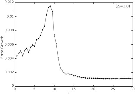
FIGURE 7. Similar to Figure 6 but for the RIC method, assuming the same set of model parameters as in Figure 6 and a fixed lead time Δ = 1.0.

Regarding the RP method, one notices somewhat different behaviors of err (τ, Δ) compared to the RIC or RF methods, depending on which model parameters are used and whether the RP method employs the initial or time-varying implementation (Figure 8). For the initial RP approach, the overall properties of err (τ, Δ) for the static stability parameter s are almost the same as those with the RF or RIC method. In other words, the maximum error growth rate occurs during the pre-conditioning period, followed by a decreasing period and level off at the MPI equilibrium (Figure 8A). In contrast, both SST and surface drag parameters show a quick increase in the error growth rate at first but then maintain a large error growth rate during the entire subsequent stage of TC development, instead of subsiding over time as for the RF or RIC method. This unique behavior of err (τ, Δ) for T _s and C _d is because the uncertainty magnitude of these parameters is much larger than that of s at the equilibrium, even though the relative percentage is the same. One can see this directly by looking at the sensitivity analyses for the initial RP method (see Supplementary Appendix S1). Apparently, the same 10% variability of each parameter would give a different absolute magnitude in the RP method. That is, a 10% variability of s would give an absolute uncertainty magnitude of 0.01, whereas the same 10% variability of T _s or C _d would result in an absolute uncertainty magnitude of 0.1. This explains the difference in the error growth rate at the mature stage, as shown in Figure 8 for the initial RP implementation.

FIGURE 8

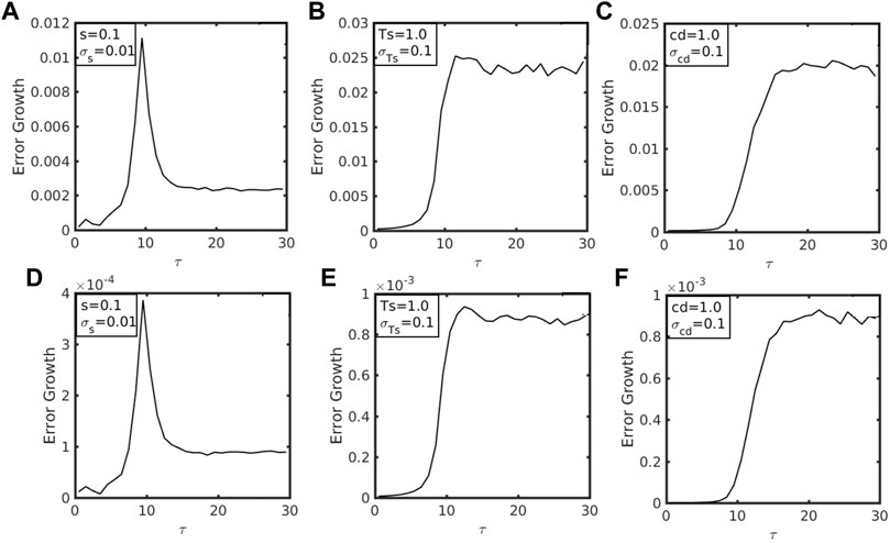
FIGURE 8. Similar to Figure 6 but for the random parameter approach with (A–C) initial RP method and (D–F) time-varying RP method.

For the time-varying RP implementation, err (τ, Δ) is about one order of magnitude smaller than what was obtained from the initial RP method. Recall that such a large difference of err (τ, Δ) between the initial and time-varying RP approaches is not unique to the rapid intensification period. However, it is, in fact, true for the MPI equilibrium as well (cf. Figure 4). This is noteworthy because it suggests that both the RF and the initial RP methods produce more intensity errors than randomizing model parameters during the course of TC development. Again, this conclusion should be cautioned because it is drawn from a simple MSD system that may or may not fully reflect real TC development. Further verification of these results in the full-physics CM1 model will be presented in the following section.

4 CM1 Model Results

Although the results obtained from the low-order MSD system are significant, various simplifications in the MSD model naturally raise the question of how much these results can be realized in real TCs. In this section, we examine similar properties of TC intensity error growth and saturation for the CM1 model, using the same random representation methods as for the MSD system. Unlike the MSD model, it should be emphasized that the CM1 model does not converge to a single MPI equilibrium (Figure 9A), even with the axisymmetric setting. Instead, CM1 reaches a statistical quasi-equilibrium state due to the possible existence of low-dimensional chaos at the MPI limit that the MSD model cannot capture, as mentioned in Section 2.2 (Kieu and Moon, 2016; Kieu et al., 2018). Thus, the MPI equilibrium must be now understood in a statistical sense for all analyses in this section.

FIGURE 9

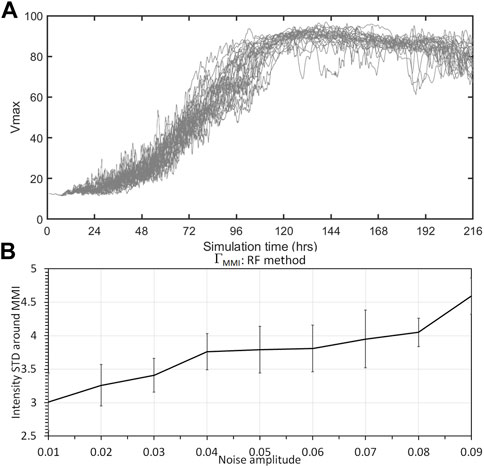
FIGURE 9. (A) Time series of the maximum tangential wind (V _MAX, unit ms ⁻¹) as obtained from 100 20-day simulations of the CM1 model that is implemented with the RF method; and (B) the standard deviation of V _MAX (unit, ms ⁻¹) at the maximum intensity equilibrium (day 9–18 into integration) as a function of the random forcing standard deviation. Error bars denote 95% confidence intervals.

4.1 Intensity Variability at the MPI Equilibrium

Figure 9B shows the standard deviation of TC intensity fluctuation (hereinafter denoted as Γ _MMI to distinguish from Γ obtained from the MSD system) as a function of noise amplitudes in the RF simulation, which is averaged during the CM1 quasi-stationary maximum intensity (MMI ² ) stage. With more realistic physics, in Figure 9B, one notices that the intensity variability tends to increase with the amplitude of stochastic forcing, similar to what was obtained from the MSD model. This result may seem at first somewhat trivial, but it is very noteworthy. Indeed, such an increase in Γ _MMI indicates that stochastic forcing can actually introduce further variability to TC intensity, even in the presence of possible low-dimensional chaos at the MMI equilibrium. Sugihara et al. (1994) (NKF) discussed that stochastic and chaotic variability are generally different because deterministic chaos can exist without any stochastic forcing. The fact that Γ _MMI increases with random noise amplitude, as shown in Figure 9B, suggests that stochastic forcing could contribute to intensity errors at long lead times beyond the chaotic dynamics if the stochastic forcing is sufficiently large.

For the RP method, different intensity variability between T _s and C _d is captured (Figure 10). For T _s , both MMI and Γ _MMI increase with SST, consistent with previous studies (Keshavamurthy and Kieu, 2021). While the increase in MMI with T _s is well understood, the increase in Γ _MMI with T _s is of note here, as it indicates that a warmer SST would also result in higher uncertainty for intensity forecast (Kieu and Moon, 2016; Keshavamurthy and Kieu, 2021).

FIGURE 10

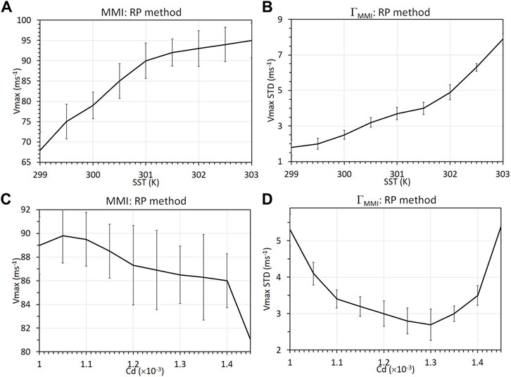
FIGURE 10. Dependence of V _MAX (left panels) and its corresponding standard deviation (right panels) on (A,B) SST and (C,D) C _d with a fixed noise amplitude in the time-varying RP method.

In contrast, the surface drag coefficient shows a decrease of MMI for a larger C _d as generally expected, yet Γ _MMI first decreases and then increases with C _d (Figure 10D). This unique behavior of intensity variability in the C _d experiment is due to the dual role of C _d in determining both the MMI and the uncertainty. In other words, when C _d increases from a small value, it will reduce both MMI and the fluctuation around the MMI due to the nature of the frictional forcing against motion. When C _d is sufficiently large, MMI is, however, too weak; it is no longer able to “trap” the intensity fluctuation. Therefore, the fluctuation of intensity around the MMI equilibrium becomes larger, as discussed in NKF.

Given such dependence of MMI and the variability around MMI on T _s and C _d in the RP method, Figures 11B–C show how Γ _MMI depends on the random noise amplitude of T _s and C _d in the CM1 model. Herein, we present results only for the initial RP approach because the time-varying RP method produces a much smaller intensity variability compared to the initial RP method in the CM1 model.

FIGURE 11

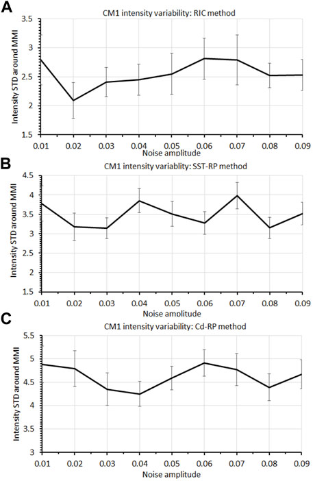
FIGURE 11. Similar to Figure 9B but for (A) the RIC method, (B) the initial RP method with a random SST parameter, and (C) the initial RP method with a random C _d parameter obtained from the CM1 model.

Unlike the MSD model, Γ _MMI does not seem to increase with the noise amplitude for the initial RP method. The same is true for the RIC method when increasing the random noise amplitude of initial conditions, capturing no change in Γ _MMI , as seen in Figure 11A. Such resilience of the intensity variability at the MMI equilibrium for both the RIC and RP methods reflects the fact that this equilibrium is not a point-like equilibrium as in the MSD model. However, it may contain a chaotic attractor of TC dynamics that randomizing model parameters or initial conditions does not help. Consequently, the fluctuation of MMI at the equilibrium is no longer linearly dependent on the random fluctuation of initial conditions or model parameters as in the MSD system. In this regard, the CM1 results shown in Figure 11 imply that long-term intensity errors in full-physics models may be subject to less of an impact caused by vortex initialization uncertainties or random model parameters/truncation errors, compared to the intrinsic variability of TC dynamics (Du et al., 2013; Kieu et al., 2021).

4.2 Intensity Error Growth

Along with the intensity error saturation, it is important to also validate the characteristics of the intensity error growth obtained from the MSD model. Unlike the MSD model, in which one can add random noise for any representation method in studying error growth, the CM1 model has strong constraints on the model design and numerical stability that prevent one from adding random noise arbitrarily. Therefore, we examine in this section the error growth in the CM1 model only for the RF and RIC methods.

Figure 12A shows the error growth rate for the RF method obtained from the CM1 model between 48 and 180 h into integration (cf. Figure 9). For this RF method, the CM1 error growth rate confirms what was obtained from the MSD model, with a larger error growth rate during rapid intensification and much slower growth during the quasi-stationary stage. Detailed comparison of Figures 9, 12 shows that the peak in the error growth rate occurs, however, around t = 72h in the CM1 model, which is after the onset of TC rapid intensification, whereas the maximum error growth in the MSD model is prior to the onset of rapid intensification (cf. Figure 7). Although this behavior of error growth in the CM1 model is difficult to be explained due to the more complex nature of TC nonlinear dynamics, it could reflect the fact that the onset of TC rapid intensification in the full-physics model is generally less well-defined than that in the MSD model in the presence of stochastic forcing. Thus, any perturbation introduced into the model may be smoothed out until the model vortex enters its rapid intensification period. Of course, this is more or less speculation at this point because there is no effective way to isolate the smoothing effect in the CM1 model. However, it highlights some difficulty when analyzing error growth in full-physics models such as CM1, which is absent in the MSD model.

FIGURE 12

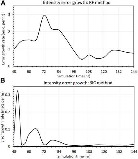
FIGURE 12. (A) Dependence of the error growth rate (unit ms ⁻¹perhr) on the stage of TC development for the 12 h lead time obtained from the RF implementation for the CM1 model; and (B) similar to (A) but for the RIC implementation.

In contrast to the RF method, the error growth in the RIC method captures somewhat more consistent growth rate characteristics compared to the MSD model, with the largest growth rate prior to the onset of rapid intensification (Figure 12B). Moreover, the growth rate also subsides over time and becomes stabilized during the MMI stage. This result also accords with the idealized experiments and real-time intensity verification presented in Kieu et al. (2018) and Keshavamurthy and Kieu (2021), thus supporting 1) larger uncertainty of intensity forecast during TC rapid intensification and 2) the existence of chaotic attractor at the MMI stage.

It should be noted again that the implementation of the RIC method in the CM1 model, by design, does not include stochastic forcing as in the RF method. Thus, the error growth in the RIC experiments with either the CM1 or the MSD model resulted merely from the spread of perturbations under the TC deterministic dynamics, which possesses more well-defined onset of rapid intensification compared to the RF implementation. In this regard, the intensity error growth in the RIC experiment shown in Figure 11 could truly reflect the behaviors of intensity variability related to the initial condition uncertainty prior to, during, and after TC rapid intensification, similar to the TC dynamics in the MSD model.

5 Conclusion

This study examined different methods to represent stochastic processes in TC development, using a fidelity-reduced TC model and a full-physics model. With the focus on TC intensity variability at the equilibrium and the intensity error growth during TC rapid intensification, several significant results have been obtained from both the theoretical and numerical perspectives.

First, our series of Monte Carlo simulations for the fidelity-reduced model based on the TC-scale dynamics (MSD) showed that the random forcing method in which the model forcing is augmented by a stochastic term results in the largest fluctuation of TC intensity at the maximum potential intensity (MPI) limit compared to randomizing either initial conditions or model parameters. In addition, the response of TC intensity to the random forcing method increases with the random noise amplitude, and it is dominated by the tangential wind and warm-core anomaly components, as reported in NKF.

Second, a similar response of TC intensity variability to random noise was also observed for the random parameter method, but the response depends sensitively on how one randomizes model parameters. For the initial random parameter approach in which the model parameters are randomized only at the initial time, TC intensity variability at the MPI limit increases almost linearly with the noise amplitude. For the time-varying random parameter method in which the model parameters are randomized every time step, the intensity fluctuation is one order of magnitude smaller than the initial random parameter method. Such behaviors of TC intensity variability at the MPI limit are consistent with those obtained from stochastic linear models and reveal the importance of how one implements random model parameters in TC models.

Regarding the intensity error growth during TC development, it was found that the error growth rate in the MSD model peaks right before the onset of rapid intensification and then gradually subsides during the intensification period before leveling off at the MPI equilibrium. This characteristic of TC intensity error growth was captured for all random representation methods, except for the initial random parameter methods with two specific parameters T _s (sea surface temperature) and C _d (the surface drag coefficient), due to their unique role in the MPI equilibrium. Specifically the random variation of these two parameters produces an overall larger intensity error growth rate at the MPI limit, which is not applied to other parameters or random methods.

Third, to verify the results obtained from the fidelity-reduced MSD model, cloud-resolving simulations with the CM1 model were conducted. By implementing the same random representation methods for the CM1 axisymmetric configuration, it was confirmed that random forcing plays the most significant role in the overall variability of TC intensity and the intensity error growth during TC development. The CM1 model experiments also confirmed that the random initial condition tends to be more effective during the early stage of TC development but becomes less significant relative to either the random parameter or random forcing method at the later stage of TC development. The findings obtained from both the MSD and CM1 models highlight the importance of choosing a proper random forcing method to represent the variability of TC intensity in operation.

Two major differences between the MSD and the CM1 model that could strongly affect the analyses of TC intensity variability should be noted here. First, unlike the MSD model, which contains a single stable MPI point with no chaos, CM1 possesses some classical chaotic behaviors at the MPI equilibrium similar to other full-physics models (Kieu and Moon, 2016; Keshavamurthy and Kieu, 2021, NKF). While the existence of this chaotic MPI attractor is still elusive, its potential existence is needed to explain the larger intensity variability in the CM1 model, even in the absence of all stochastic forcings. The results shown in Figure 11 may therefore display the variability of TC intensity due mostly to chaotic dynamics rather than purely random noise as discussed in NKF. The relative contribution between chaotic and stochastic variability is unknown at present, as the CM1 model does not allow for large random noise amplitudes.

The second difference between MSD and CM1 is that the maximum intensity equilibrium in CM1 is sensitive to model configuration and physical parameterizations that may or may not be maintained during arbitrarily long simulation. Unlike the low-order MSD model for which a fixed environment is always assumed, CM1 simulates a TC vortex in a finite domain. Without proper physical schemes such as radiative parameterization or lateral boundary condition adjustment, the model domain will be eventually affected by the subsidence warming in the outer region, thus changing the TC environment and causing the model to spin down. In this regard, the analyses of TC intensity at the maximum intensity equilibrium contain some uncertainty that one has to resolve in future studies before a more definite conclusion of intrinsic TC intensity variability can be obtained.

Data Availability Statement

The original contributions presented in the study are included in the article/Supplementary Material. Further inquiries can be directed to the corresponding author.

Author Contributions

CK perceived the idea and designed experiments. W-TLF carried out mathematical analyses. MP performed simulations and analyses. All authors contributed to the writing of the manuscript.

Funding

This research was partially supported by ONR Awards N000141812588.

Conflict of Interest

The authors declare that the research was conducted in the absence of any commercial or financial relationships that could be construed as a potential conflict of interest.

Publisher’s Note

All claims expressed in this article are solely those of the authors and do not necessarily represent those of their affiliated organizations or those of the publisher, the editors, and the reviewers. Any product that may be evaluated in this article, or claim that may be made by its manufacturer, is not guaranteed or endorsed by the publisher.

Acknowledgments

CK wishes to thank the NOAA Geophysical Fluid Dynamics Laboratory and Princeton University for their support and hospitality during the sabbatical period that this work was prepared. The authors wish to also thank two anonymous reviewers for their suggestions and comments, which have helped improve this work.

Supplementary Material

The Supplementary Material for this article can be found online at: https://www.frontiersin.org/articles/10.3389/feart.2022.893781/full#supplementary-material

Footnotes

¹ Technically, this property is related to the fact that the MSD model can be treated as an extended Markov system (u, v, b, s, T _s , C _d ). For this extended system, one first obtains the stationary distribution μ by solving the equation ${\mathcal{L}}^{\ast }\mu =0$ for the stationary distribution μ, where ${\mathcal{L}}^{\ast }$ is the adjoint of the generator $\mathcal{L}$ of the Markovian system. Then, the error growth at a large time limit can be approximated by the standard deviation of the v-component under the stationary distribution.

² It should be noted that the actual CM1 model maximum intensity (MMI) is generally different from the theoretical MPI value.

References

Aberson, S. D., Aksoy, A., Sellwood, K. J., Vukicevic, T., and Zhang, X. (2015). Assimilation of High-Resolution Tropical Cyclone Observations with an Ensemble Kalman Filter Using HEDAS: Evaluation of 2008–11 HWRF Forecasts. Mon. Wea. Rev. 143, 511–523. doi:10.1175/mwr-d-14-00138.1

CrossRef Full Text | Google Scholar

Aksoy, A., Aberson, S. D., Vukicevic, T., Sellwood, K. J., Lorsolo, S., and Zhang, X. (2013). Assimilation of High-Resolution Tropical Cyclone Observations with an Ensemble Kalman Filter Using NOAA/AOML/HRD’s HEDAS: Evaluation of the 2008–11 Vortex-Scale Analyses. Mon. Wea. Rev. 141, 1842–1865. doi:10.1175/mwr-d-12-00194.1

CrossRef Full Text | Google Scholar

Arakawa, A., and Schubert, W. H. (1974). Interaction of a Cumulus Cloud Ensemble with the Large-Scale Environment, Part I. J. Atmos. Sci. 31, 674–701. doi:10.1175/1520-0469(1974)031<0674:ioacce>2.0.co;2

CrossRef Full Text | Google Scholar

Breil, M., and Schädler, G. (2017). Quantification of the Uncertainties in Soil and Vegetation Parameterizations for Regional Climate Simulations in Europe. J. Hydrometeorol. 18, 1535–1548. doi:10.1175/JHM-D-16-0226.1

CrossRef Full Text | Google Scholar

Brown, B. R., and Hakim, G. J. (2013). Variability and Predictability of a Three-Dimensional Hurricane in Statistical Equilibrium. J. Atmos. Sci. 70, 1806–1820. doi:10.1175/JAS-D-12-0112.1

CrossRef Full Text | Google Scholar

Bryan, G. H., and Fritsch, J. M. (2002). A Benchmark Simulation for Moist Nonhydrostatic Numerical Models. Mon. Wea. Rev. 130, 2917–2928. doi:10.1175/1520-0493(2002)130<2917:absfmn>2.0.co;2

CrossRef Full Text | Google Scholar

Christensen, H. M. (2020). Constraining Stochastic Parametrisation Schemes Using High‐resolution Simulations. Q.J.R. Meteorol. Soc. 146, 938–962. doi:10.1002/qj.3717

CrossRef Full Text | Google Scholar

Christensen, H. M., Moroz, I. M., and Palmer, T. N. (2015). Stochastic and Perturbed Parameter Representations of Model Uncertainty in Convection Parameterization*. J. Atmos. Sci. 72, 2525–2544. doi:10.1175/jas-d-14-0250.1

CrossRef Full Text | Google Scholar

Doblas-Reyes, F. J., Weisheimer, A., Déqué, M., Keenlyside, N., McVean, M., Murphy, J. M., et al. (2009). Addressing Model Uncertainty in Seasonal and Annual Dynamical Ensemble Forecasts. Q. J. R. Meteorol. Soc. 135, 1538–1559. doi:10.1002/qj.464

CrossRef Full Text | Google Scholar

Dorrestijn, J., Crommelin, D. T., Siebesma, A. P., and Jonker, H. J. J. (2015). Stochastic Parameterization of Convective Area Fractions with a Multicloud Model Inferred from Observational Data. J. Atmos. Sci. 72, 854–869. doi:10.1175/jas-d-14-0110.1

CrossRef Full Text | Google Scholar

Du, T. D., Ngo-Duc, T., Hoang, M. T., and Kieu, C. Q. (2013). A Study of Connection between Tropical Cyclone Track and Intensity Errors in the Wrf Model. Meteor. Atmos. Phys. 122, 55–64. doi:10.1007/s00703-013-0278-0

CrossRef Full Text | Google Scholar

Fan, W.-T., Jolly, M., and Pakzad, A. (2021a). Three-dimensional Shear Driven Turbulence with Noise at the Boundary. Nonlinearity 34, 4764–4786. doi:10.1088/1361-6544/abf84b

CrossRef Full Text | Google Scholar

Fan, W.-T., Kieu, C., Sakellariou, D., and Patra, M. (2021b). Hitting Time of Rapid Intensification Onset in Hurricane-like Vortices. Phys. Fluids 33, 096603. doi:10.1063/5.0062119

CrossRef Full Text | Google Scholar

Gopalakrishnan, S. G., Marks, F., Zhang, X., Bao, J.-W., Yeh, K.-S., and Atlas, R. (2011). The Experimental HWRF System: A Study on the Influence of Horizontal Resolution on the Structure and Intensity Changes in Tropical Cyclones Using an Idealized Framework. Mon. Wea. Rev. 139, 1762–1784. doi:10.1175/2010mwr3535.1

CrossRef Full Text | Google Scholar

Hakim, G. J. (2011). The Mean State of Axisymmetric Hurricanes in Statistical Equilibrium. J. Atmos. Sci. 68, 1364–1376. doi:10.1175/2010jas3644.1

CrossRef Full Text | Google Scholar

Halperin, D. J., and Torn, R. D. (2018). Diagnosing Conditions Associated with Large Intensity Forecast Errors in the Hurricane Weather Research and Forecasting (HWRF) Model. Weather Forecast. 33, 239–266. doi:10.1175/WAF-D-17-0077.1

CrossRef Full Text | Google Scholar

Hamill, T. M., Whitaker, J. S., Kleist, D. T., Fiorino, M., and Benjamin, S. G. (2011). Predictions of 2010's Tropical Cyclones Using the GFS and Ensemble-Based Data Assimilation Methods. Mon. Wea. Rev. 139, 3243–3247. doi:10.1175/mwr-d-11-00079.1

CrossRef Full Text | Google Scholar

Kain, J. S., and Fritsch, J. M. (1990). A One-Dimensional Entraining/detraining Plume Model and its Application in Convective Parameterization. J. Atmos. Sci. 47, 2784–2802. doi:10.1175/1520-0469(1990)047<2784:aodepm>2.0.co;2

CrossRef Full Text | Google Scholar

Keshavamurthy, K., and Kieu, C. (2021). Dependence of Tropical Cyclone Intrinsic Intensity Variability on the Large‐scale Environment. Q.J.R. Meteorol. Soc. 147, 1606–1625. doi:10.1002/qj.3984

CrossRef Full Text | Google Scholar

Kieu, C., Evans, C., Jin, Y., Doyle, J. D., Jin, H., and Moskaitis, J. (2021). Track Dependence of Tropical Cyclone Intensity Forecast Errors in the COAMPS-TC Model. Weather Forecast. 36, 469–485. doi:10.1175/waf-d-20-0085.1

CrossRef Full Text | Google Scholar

Kieu, C. (2015). Hurricane Maximum Potential Intensity Equilibrium. Q.J.R. Meteorol. Soc. 141, 2471–2480. doi:10.1002/qj.2556

CrossRef Full Text | Google Scholar

Kieu, C., Keshavamurthy, K., Tallapragada, V., Gopalakrishnan, S., and Trahan, S. (2018). On the Growth of Intensity Forecast Errors in the Operational Hurricane Weather Research and Forecasting (HWRF) Model. Q. J. R. Meteorol. Soc. 144, 1803–1819. doi:10.1002/qj.3344

CrossRef Full Text | Google Scholar

Kieu, C. Q., and Moon, Z. (2016). Hurricane Intensity Predictability. Bull. Amer. Meteor. Soc. 97, 1847–1857. doi:10.1175/BAMS-D-15-00168.1

CrossRef Full Text | Google Scholar

Kieu, C. Q., and Wang, Q. (2018). On the Scale Dynamics of the Tropical Cyclone Intensity. Discrete Continuous Dyn. Syst. - B 23, 3047. doi:10.3934/dcdsb.2017196

CrossRef Full Text | Google Scholar

Kieu, C., and Wang, Q. (2017). Stability of the Tropical Cyclone Intensity Equilibrium. J. Atmos. Sci. 74, 3591–3608. doi:10.1175/jas-d-17-0028.1

CrossRef Full Text | Google Scholar

Kurihara, Y., Bender, M. A., Tuleya, R. E., and Ross, R. J. (1995). Improvements in the GFDL Hurricane Prediction System. Mon. Wea. Rev. 123, 2791–2801. doi:10.1175/1520-0493(1995)123<2791:iitghp>2.0.co;2

CrossRef Full Text | Google Scholar

Liu, Q., Marchok, T., Pan, H., Bender, M., and Lord, S. (2000). Improvements in Hurricane Initialization and Forecasting at Ncep with Global and Regional (GFDL) Models. Proced. Bull. 472. NCEP/EMC. [Available at NOAA/NWS, 1325 East–West Highway, Silver Spring, MD 20910 at: http://205.156.54.206/om/tpb/472.htm.

Google Scholar

Nguyen, P., Kieu, C., and Fan, W.-T. L. (2020). Stochastic Variability of Tropical Cyclone Intensity at the Maximum Potential Intensity Equilibrium. J. Atmos. Sci. 77(9), 3105–3118. doi:10.1175/jas-d-20-0070.1

CrossRef Full Text | Google Scholar

Palmer, T. N. (2001). A Nonlinear Dynamical Perspective on Model Error: A Proposal for Non-local Stochastic-Dynamic Parametrization in Weather and Climate Prediction Models. Q.J R. Met. Soc. 127, 279–304. doi:10.1002/qj.49712757202

CrossRef Full Text | Google Scholar

Palmer, T. N. (2012). Towards the Probabilistic Earth-System Simulator: A Vision for the Future of Climate and Weather Prediction. Q.J.R. Meteorol. Soc. 138, 841–861. doi:10.1002/qj.1923

CrossRef Full Text | Google Scholar

Plant, R. S., and Craig, G. C. (2008). A Stochastic Parameterization for Deep Convection Based on Equilibrium Statistics. J. Atmos. Sci. 65, 87–105. doi:10.1175/2007jas2263.1

CrossRef Full Text | Google Scholar

Rappin, E. D., Nolan, D. S., and Majumdar, S. J. (2013). A Highly Configurable Vortex Initialization Method for Tropical Cyclones. Mon. Weather Rev. 141, 3556–3575. doi:10.1175/MWR-D-12-00266.1

CrossRef Full Text | Google Scholar

Richter, D. H., Wainwright, C., Stern, D. P., Bryan, G. H., and Chavas, D. (2021). Potential Low Bias in High-Wind Drag Coefficient Inferred from Dropsonde Data in Hurricanes. J. Atmos. Sci. 78, 2339–2352. doi:10.1175/JAS-D-20-0390.1

CrossRef Full Text | Google Scholar

Song, Y., Wikle, C. K., Anderson, C. J., and Lack, S. A. (2007). Bayesian Estimation of Stochastic Parameterizations in a Numerical Weather Forecasting Model. Mon. Weather Rev. 135, 4045–4059. doi:10.1175/2007MWR1928.1

CrossRef Full Text | Google Scholar

Sugihara, G., Grenfell, B. T., May, R. M., and Tong, H. (1994). Nonlinear Forecasting for the Classification of Natural Time Series. Phil. Trans. R. Soc. Lond. A 348, 477–495. doi:10.1098/rsta.1994.0106

CrossRef Full Text | Google Scholar

Suhas, E., and Zhang, G. J. (2014). Evaluation of Trigger Functions for Convective Parameterization Schemes Using Observations. J. Clim. 27, 7647–7666. doi:10.1175/jcli-d-13-00718.1

CrossRef Full Text | Google Scholar

Tallapragada, V., Bernardet, L., Gopalakrishnan, S., Kwon, Y., Liu, Q., Marchok, T., et al. (2012). Hurricane Weather Research and Forecasting (HWRF) Model: 2012 Scientific Documentation. Dev. Testbed Cent. 142(11), 4308–4325. doi:10.1175/MWR-D-13-00010.1

CrossRef Full Text | Google Scholar

Tong, M., Sippel, J. A., Tallapragada, V., Liu, E., Kieu, C., Kwon, I.-H., et al. (2018). Impact of Assimilating Aircraft Reconnaissance Observations on Tropical Cyclone Initialization and Prediction Using Operational HWRF and GSI Ensemble-Variational Hybrid Data Assimilation. Mon. Weather Rev. 146, 4155–4177. doi:10.1175/MWR-D-17-0380.1

CrossRef Full Text | Google Scholar

Trabing, B. C., and Bell, M. M. (2020). Understanding Error Distributions of Hurricane Intensity Forecasts during Rapid Intensity Changes. Weather Forecast. 35, 2219–2234. doi:10.1175/WAF-D-19-0253.1

CrossRef Full Text | Google Scholar

Van Nguyen, H., and Chen, Y.-L. (2011). High-resolution Initialization and Simulations of Typhoon Morakot (2009). Mon. Wea. Rev. 139, 1463–1491. doi:10.1175/2011mwr3505.1

CrossRef Full Text | Google Scholar

Weisheimer, A., Palmer, T. N., and Doblas-Reyes, F. J. (2011). Assessment of Representations of Model Uncertainty in Monthly and Seasonal Forecast Ensembles. Geophys. Res. Lett. 38, a–n. doi:10.1029/2011GL048123

CrossRef Full Text | Google Scholar

Zhang, F., and Weng, Y. (2015). Predicting Hurricane Intensity and Associated Hazards: A Five-Year Real-Time Forecast Experiment with Assimilation of Airborne Doppler Radar Observations. Bull. Amer. Meteor. Soc. 96, 25–33. doi:10.1175/bams-d-13-00231.1

CrossRef Full Text | Google Scholar

Zhang, J. A. (2010). Estimation of Dissipative Heating Using Low-Level In Situ Aircraft Observations in the Hurricane Boundary Layer. J. Atmos. Sci. 67, 1853–1862. doi:10.1175/2010jas3397.1

CrossRef Full Text | Google Scholar

Zhang, J. A., Marks, F. D., Montgomery, M. T., and Lorsolo, S. (2011). An Estimation of Turbulent Characteristics in the Low-Level Region of Intense Hurricanes Allen (1980) and Hugo (1989). Mon. Wea. Rev. 139, 1447–1462. doi:10.1175/2010MWR3435.1

CrossRef Full Text | Google Scholar

Zhang, Z., Tallapragada, V., Kieu, C., Trahan, S., and Wang, W. (2015). HWRF Based Ensemble Prediction System Using Perturbations from GEFS and Stochastic Convective Trigger Function. Trop. Cyclone Res. Rev. 3, 145–161. doi:10.6057/2014TCRR03.02

CrossRef Full Text | Google Scholar

Zou, X., and Tian, X. (2018). Hurricane Warm‐Core Retrievals from AMSU‐A and Remapped ATMS Measurements with Rain Contamination Eliminated. J. Geophys. Res. Atmos. 123, 829. doi:10.1029/2018JD028934

CrossRef Full Text | Google Scholar