Gradient normalized least-squares reverse-time migration imaging technology

Least-squares reverse-time migration (LSRTM) can overcome the problems of low resolution and unbalanced amplitude energy of deep formation imaging in reverse-time migration (RTM); hence, it can obtain a more accurate imaging profile. In the conventional conjugate gradient LSRTM, the gradient is obtained based on cross correlation without a precondition operator, and the source has a great influence on the gradient, causing the convergence rate to be slow. In the framework of conventional conjugate gradient LSRTM, a normalized cross-correlation of the source wavefield was used in this study to effectively weaken the influence of the source effect and reduce the low-frequency noise. The idea of normalized cross-correlation of the source wavefield was adopted to improve the steepest descent gradient to further accelerate the iterative convergence speed and complete the final migration imaging. Model and field data examples verify the advantages of the proposed methods over conventional methods in reducing source effects, improving convergence speed, and enhancing underground deep illumination.

Introduction

Reverse-time migration (RTM) is considered the most accurate imaging technology used in complex structure imaging (Baysal et al., 1983). It employs the numerical solution of the two-way wave equation to reverse continuation seismic records, and it can process imaging of strong velocity variation and steep dip angles. Because of the conventional RTM, cross-correlation imaging is the result of migration operator transposition rather than its inverse and limited acquisition aperture, complex underground structure, and limited seismic bandwidth. RTM can only provide fuzzy structural information, and therefore, it cannot obtain accurate imaging results (Claerbout, 1992), which cannot carry out fine imaging of complex oil and gas reservoirs. Least-squares reverse-time migration (LSRTM) is a true-amplitude imaging method based on linear inversion theory, which was first introduced into seismic inversion by Bamberger et al. (1982). Later, Tarantola (1984) proposed the theoretical framework of least-squares inversion. Furthermore, many experts and scholars have continuously improved the LSRTM and applied it to the field data. Nemeth et al. (1999) proposed the least-squares Kirchhoff migration method for irregular seismic data (such as trace missing and sampling irregular data) to eliminate the migration artifacts caused by irregular data. Although it has the above-mentioned advantage, the calculation accuracy of Kirchhoff wave field propagator is low and cannot meet the requirements of actual production. Kuehl and Sacchi (2001a, 2003) proposed the introduction of the least-squares migration into the wave field propagator, and subsequent studies mainly focused on the areas such as rapid calculation of the Hessian matrix, the improvement of imaging resolution, regularization constraints, and the improvement of computing efficiency. Yang and Zhang (2008) adopted Fourier finite-difference migration and forward operator to carry out post-stack least-squares migration, to eliminate imaging noise to a certain extent and improve resolution. Wang et al. (2009) developed a new iterative regularization model of migration inversion imaging and proposed a hybrid conjugate gradient algorithm to solve the model. Huang et al.(2013a, 2013b) achieved good inversion results by using least-squares Kirchhoff migration algorithm for model and field data testing. Furthermore, Guo et al. (2015) realized iterative LSRTM imaging by employing the research of error functional establishment, RTM data reconstruction algorithm, Hessian reverse regularization gradient calculation, and established the implementation process of LSRTM for field data. Huang et al. (2015) studied the theoretical method and the processing process of LSRTM based on static plane wave coding. The test results showed that this method could effectively suppress the low-frequency imaging noise and crosstalk noise, and compensate deep imaging energy, which was an effective amplitude-preserved imaging strategy.

Although the LSRTM has obvious advantages, there are still many problems encountered when it is applied to field data. On the one hand, the LSRTM is computationally inefficient. On the other hand, because the actual source wavelet is difficult to estimate, the conventional conjugate gradient method has a great influence on obtaining the source energy, and it is difficult to obtain the Hessian inverse, resulting in the imbalance of underground deep illumination (Zhang et al., 2013). To solve these problems, geophysicists began to construct preconditioned operators to approximate the Hessian inverse and to preprocess the gradient, including damping constraints (Tarantola, 1984), focusing or smoothness constraints of common imaging point gathers (Kuehl and Sacchi, 2001b; Prucha and Biondi, 2002), dip angle constraint condition (Prucha and Biondi, 2002), prediction operator (Wang et al., 2003), defuzzification operator (Aoki and Schuster, 2009), and sparse transform constraints, using the sparse distribution characteristics of imaging results in the wavelet or curvelet domains to constrain (Herrmann et al., 2019).

When there is no suitable precondition operator in the gradient computation of conventional conjugate gradient LSRTM, the source effect will lead to serious interference with the migration result, resulting in shallow energy concentration, insufficient illumination in deep layers, and slow convergence rate of the iterative process. Normalization can solve the source effect problem in RTM well. In this study, the source normalization was introduced into the gradient optimization process to weaken the influence of the source effect, accelerate the convergence speed of the algorithm, and obtain the final LSRTM imaging.

Methods

Born approximation

The constant density acoustic wave equation is

$\left({\mathbf{\nabla }}^2-\frac{\mathbf{1}}{{\mathit{v}}^{\mathbf{2}}\left(\mathit{X}\right)}\frac{{\mathbf{\partial }}^{\mathbf{2}}}{{\mathbf{\partial }}^{\mathbf{2}}\mathit{t}}\right)\mathit{p}=\mathit{\delta }\left(\mathit{X-}{\mathit{X}}_{\mathit{s}}\right)\mathit{\delta }\left(\mathit{t}\right)(1)$

where p is the wave field function, v(X) is the velocity at the X position, and the X_s and X are the position of the source and the geophone, respectively.

The actual velocity field can be composed of normal field and disturbance:

$\frac{\mathbf{1}}{{\mathit{v}}^{\mathbf{2}}\left(\mathit{X}\right)}=\frac{\mathbf{1}}{{\mathit{v}}_{\mathbf{0}}^{\mathbf{2}}\left(\mathit{X}\right)}\left(\mathbf{1}-\mathit{\alpha }\left(\mathit{X}\right)\right)(2)$

By expanding Taylor’s Eq. 2 at v₀ and removing the higher order term, we obtain the following result:

$\frac{\mathbf{1}}{{\mathit{v}}_{\mathbf{0}}^{\mathbf{2}}}-\frac{\mathbf{2}\mathbf{\Delta }\mathit{v}}{{\mathit{v}}_{\mathbf{0}}^{\mathbf{3}}}=\frac{\mathbf{1}}{{\mathit{v}}_{\mathbf{0}}^{\mathbf{2}}}\left(\mathbf{1}-\mathit{\alpha }\right)(3)$

where $\mathit{\alpha }=\frac{2\mathrm{\Delta }\mathit{v}}{{\mathit{v}}_0}$, α(X) is the disturbance. After applying Eq. 2 into (1), and transforming the equation into Fourier frequency domain, we have

$\left[{\mathit{\nabla }}^{\mathbf{2}}+\frac{{\mathit{\omega }}^{\mathbf{2}}}{{\mathit{v}}_{\mathbf{0}}^{\mathbf{2}}}\left(\mathbf{1}-\mathit{\alpha }\left(\mathit{X}\right)\right)\right]\mathit{P}\left(\mathit{X},{\mathit{X}}_{\mathit{S}},\mathit{\omega }\right)=\mathit{\delta }\left(\mathit{X}-{\mathit{X}}_{\mathit{S}}\right)(4)$

where $\mathit{P}\left(\mathit{X},{\mathit{X}}_{\mathit{S}},\mathit{\omega }\right)={\displaystyle \underset{-\mathit{\infty }}{\overset{\mathit{\infty }}{\int }}\mathit{p}\left(\mathit{X},{\mathit{X}}_{\mathit{S}},\mathit{t}\right)}{\mathit{e}}^{-\mathit{j\omega t}}\mathit{dt}$.

By expanding Eq. 4,

$\left({\mathit{\nabla }}^{\mathbf{2}}+\frac{{\mathit{\omega }}^{\mathbf{2}}}{{\mathit{v}}_{\mathbf{0}}^{\mathbf{2}}}\right)\mathit{P}\left(\mathit{X},{\mathit{X}}_{\mathit{S}},\mathit{\omega }\right)=\mathit{\delta }\left(\mathit{X}-{\mathit{X}}_{\mathit{S}}\right)+\frac{{\mathit{\omega }}^{\mathbf{2}}}{{\mathit{v}}_{\mathbf{0}}^{\mathbf{2}}}\mathit{\alpha }\left(\mathit{X}\right)\mathit{P}\left(\mathit{X},{\mathit{X}}_{\mathit{S}},\mathit{\omega }\right)(5)$

The total observed wavefield is the sum of the incident field and the scattered field:

$\mathit{P}\left(\mathit{X},{\mathit{X}}_{\mathit{S}},\mathit{\omega }\right)={\mathit{P}}_{\mathit{0}}\left(\mathit{X},{\mathit{X}}_{\mathit{S}},\mathit{\omega }\right)+{\mathit{P}}_{\mathit{S}}\left(\mathit{X},{\mathit{X}}_{\mathit{S}},\mathit{\omega }\right)(6)$

Applying Eq. 6 into (5) and decomposing it into two formulas:

$\left({\mathbf{\nabla }}^{\mathbf{2}}+\frac{{\mathit{\omega }}^{\mathbf{2}}}{{\mathit{v}}_{\mathbf{0}}^{\mathbf{2}}}\right){\mathit{P}}_{\mathit{0}}\left(\mathit{X},{\mathit{X}}_{\mathit{S}},\mathit{\omega }\right)=\mathit{\delta }\left(\mathit{X}-{\mathit{X}}_{\mathit{S}}\right)(7)$

$\left({\mathbf{\nabla }}^{\mathbf{2}}+\frac{{\mathit{\omega }}^{\mathbf{2}}}{{\mathit{v}}_{\mathbf{0}}^{\mathbf{2}}}\right){\mathit{P}}_{\mathit{S}}\left(\mathit{X},{\mathit{X}}_{\mathit{S}},\mathit{\omega }\right)=\frac{{\mathit{\omega }}^{\mathbf{2}}}{{\mathit{v}}_{\mathbf{0}}^{\mathbf{2}}}\mathit{\alpha }\left(\mathit{X}\right)\mathit{P}\left(\mathit{X},{\mathit{X}}_{\mathit{S}},\mathit{\omega }\right)(8)$

where P₀ is the background field and P_s is the scattering disturbance field. The total wavefield can be written as

$\mathit{P}\left(\mathit{X},{\mathit{X}}_{\mathit{S}},{\omega }\right)={\mathit{P}}_{\mathit{0}}\left(\mathit{X},{\mathit{X}}_{\mathit{S}},\mathit{\omega }\right)+{\displaystyle {\iiint }_{\mathit{V}}{\mathit{P}}_{\mathit{0}}\left(\mathit{X},\mathit{X}\prime ,\mathit{\omega }\right)}\frac{{\mathit{\omega }}^{\mathbf{2}}}{{\mathit{v}}_{\mathbf{0}}^{\mathbf{2}}}\mathit{\alpha }\left(\mathit{X}\right)\mathit{P}\left(\mathit{X},\mathit{X}\prime ,\mathit{\omega }\right)\mathit{dX}\prime (9)$

where V is the target region of velocity variation. Eq. 9 is the Lippmann–Schwinger integral formula. Assuming α is small, the scattering wave field under Born approximation (Liu, 2008) is expressed by:

${\mathit{P}}_{\mathit{S}}\left(\mathit{X},{\mathit{X}}_{\mathit{S}},\mathit{\omega }\right)={\displaystyle {\iiint }_{\mathit{V}}{\mathit{P}}_{\mathit{0}}\left(\mathit{X},\mathit{X}\prime ,\mathit{\omega }\right)}\frac{{\mathit{\omega }}^{\mathbf{2}}}{{\mathit{v}}_{\mathbf{0}}^{\mathbf{2}}}\mathit{\alpha }\left(\mathit{X}\right)\mathit{P}\left(\mathit{X},{X}\prime ,\mathit{\omega }\right)\mathit{dX}\prime (10)$

Defining $\mathit{m}\left(\mathit{X}\right)=\frac{2\mathrm{\Delta }\mathit{v}}{{\mathit{v}}_0^3}$ to replace α(X) in Eq. 10, the wavefield in Eq. 10 can be obtained from Eqs. 11 and 12 as

$\left({\mathbf{\nabla }}^{\mathbf{2}}+\frac{{\mathit{\omega }}^{\mathbf{2}}}{{\mathit{v}}_{\mathbf{0}}^{\mathbf{2}}}\right){\mathit{P}}_{\mathit{0}}\left(\mathit{X},{\mathit{X}}_{\mathit{S}},\mathit{\omega }\right)=\mathit{\delta }\left(\mathit{X},{\mathit{X}}_{\mathit{S}}\right)(11)$

$\left({\mathbf{\nabla }}^{\mathbf{2}}+\frac{{\mathit{\omega }}^{\mathbf{2}}}{{\mathit{v}}_{\mathbf{0}}^{\mathbf{2}}}\right){\mathit{P}}_{\mathit{S}}\left(\mathit{X},{\mathit{X}}_{\mathit{S}},\mathit{\omega }\right)={\mathit{\omega }}^{\mathbf{2}}\mathit{m}\left(\mathit{X}\right){\mathit{P}}_{\mathit{0}}\left(\mathit{X},{\mathit{X}}_{\mathit{S}},\mathit{\omega }\right)(12)$

The Born forward operator is represented by vector matrix:

$\mathit{d}=\mathit{Lm}(13)$

where m is the matrix form of migration profile or reflection coefficient model, d is the matrix form of simulation data, and L is the Born approximate forward operator matrix. The calculation of scattering wavefield can be obtained by forward simulation of Eqs. 11 and 12.

Conjugate gradient least-squares reverse-time migration

Conventional RTM can be expressed as

${\mathit{m}}_{\mathbf{0}}\left(\mathit{x},\mathit{z}\right)={\mathit{L}}^{\mathit{T}}\mathit{D}(14)$

where m₀ is the RTM profile, and L^T is the approximate migration operator. There are some errors when replacing the migration operator with the transpose of the forward modeling operator. To minimize the difference between the simulated data and the field data, the error function is defined as

$\mathit{f}\left(\mathit{m}\right)=\frac{\mathbf{1}}{\mathbf{2}}{\Vert \mathit{Lm}-\mathit{D}\Vert }^{\mathbf{2}}(15)$

After taking partial derivative with respect to m,

$\mathbf{g}=\frac{\mathbf{\partial }\mathit{f}\left(\mathit{m}\right)}{\mathbf{\partial }\mathit{m}}={\mathit{L}}^{\mathit{T}}\left(\mathit{Lm}-\mathit{D}\right)(16)$

When the gradient g is zero, the optimal solution of the least-squares problem is obtained:

$\mathit{m}={\left({\mathit{L}}^{\mathit{T}}\mathit{L}\right)}^{-\mathbf{1}}{\mathit{L}}^{\mathit{T}}\mathit{D}(17)$

where L^TL is the Hessian matrix. Because it is so large and difficult to obtain, the gradient is gradually close to zero by iteration to avoid getting the inverse of Hessian matrix.

The cross-correlation conjugate gradient method for solving Eq. 15 can be expressed as (Huang et al., 2016):

$\begin{array}{c}{\mathit{g}}^{\left(\mathit{k}+\mathbf{1}\right)}={\mathit{L}}^{\mathit{T}}\left[\mathit{L}{\mathit{m}}^{\left(\mathit{k}\right)}-\mathit{D}\right]\\ \mathit{\beta }=\frac{{\mathit{g}}^{\left(\mathit{k}+\mathbf{1}\right)}{\mathit{g}}^{\left(\mathit{k}+\mathbf{1}\right)}}{{\mathit{g}}^{\left(\mathit{k}\right)}{\mathit{g}}^{\left(\mathit{k}\right)}}\\ {\mathit{z}}^{\left(\mathit{k}+\mathbf{1}\right)}={\mathit{g}}^{\left(\mathit{k}+\mathbf{1}\right)}+\mathit{\beta }{\mathit{z}}^{\left(\mathit{k}\right)}\\ \mathit{\alpha }=\frac{{\left[{\mathit{z}}^{\left(\mathit{k}+\mathbf{1}\right)}\right]}^{\mathit{T}}{\mathit{g}}^{\left(\mathit{k}+\mathbf{1}\right)}}{{\left[\mathit{L}{\mathit{z}}^{\left(\mathit{k}+\mathbf{1}\right)}\right]}^{\mathit{T}}\mathit{L}{\mathit{z}}^{\left(\mathit{k}+\mathbf{1}\right)}}\\ {\mathit{m}}^{\left(\mathit{k}+\mathbf{1}\right)}={\mathit{m}}^{\left(\mathit{k}\right)}-\mathit{\alpha }{\mathit{z}}^{\left(\mathit{k}+\mathbf{1}\right)}\end{array}(18)$

The gradient g expansion based on the steepest descent method can be expressed as

$\mathit{g}={\displaystyle \sum _{\mathit{t}}\frac{\mathbf{\partial }{\mathit{S}}_{\mathit{s}}\left(\mathit{t},\mathit{x},\mathit{z}\right)}{\mathbf{\partial }\mathit{t}}}{\mathit{R}}_{\mathit{res}}\left(\mathit{t},\mathit{x},\mathit{z}\right)(19)$

where β is the correction factor of the conjugate gradient method, α is the update step, z is the conjugate gradient, $\mathit{g}$ is the steepest descent gradient, D is the field data, ${\mathit{S}}_{\mathit{s}}$ is the source forward wave field, and ${\mathit{R}}_{\mathit{res}}$ is the backward wavefield of the residual error between Born approximate forward data and field data.

It can be seen from Eq. 18 that the difficulty of conjugate gradient LSRTM method lies in gradient calculation and Born approximate forward modeling.

${\mathit{d}}_{\mathit{res}}=\mathit{L}{\mathit{m}}^{\left(\mathit{k}\right)}-\mathit{D}(20)$

d_res is the residual of Born approximate forward data and field data. The calculation of the steepest descent gradient is similar to the cross-correlation of conventional RTM, except that conventional RTM is the cross-correlation of field data and forward wavefield, while the steepest descent gradient is the cross-correlation of the forward modeling wave field. In the conventional cross-correlation RTM, because of the use of an imprecise migration operator, the unbalanced wave field energy affects the imaging results. When it is close to the source and geophone with strong energy, the signal may become blurred (Yang et al., 2018). To weaken the influence of energy imbalance, the imaging conditions of source-normalized cross-correlation RTM for compensating underground illumination were proposed. Considering that the preconditioner in LSRTM of conjugate gradient method is difficult to obtain and cannot approximate the Hessian matrix well, the source effect has a great impact on the gradient. Here, the normalization is used to improve the calculation process of the steepest descent gradient and weaken the influence of the source effect.

The source-normalized cross-correlation imaging condition of the RTM source is

${\mathit{m}}_{\mathbf{0}}\left(\mathit{x},\mathit{z}\right)=\frac{{\displaystyle {\sum }_{\mathit{t}}{\mathit{S}}_{\mathit{s}}\left(\mathit{t},\mathit{x},\mathit{z}\right)}{\mathit{R}}_{\mathit{s}}\left(\mathit{t},\mathit{x},\mathit{z}\right)}{{\displaystyle {\sum }_{\mathit{t}}{\left({\mathit{S}}_{\mathit{s}}\left(\mathit{t},\mathit{x},\mathit{z}\right)\right)}^{\mathbf{2}}}}(21)$

where R_S is the reverse propagation field of seismic record.

Likewise, the source-normalized steepest descent gradient formula of LSRTM is

${\tilde{\mathit{g}}}^{\left(\mathit{k}+\mathbf{1}\right)}=\frac{{\displaystyle {\sum }_{\mathit{t}}\frac{\mathbf{\partial }{\mathit{S}}_{\mathit{s}}\left(\mathit{t},\mathit{x},\mathit{z}\right)}{\mathbf{\partial }\mathit{t}}}{\mathit{R}}_{\mathit{res}}\left(\mathit{t},\mathit{x},\mathit{z}\right)}{{\displaystyle {\sum }_{\mathit{t}}{\left(\frac{\mathbf{\partial }{\mathit{S}}_{\mathit{s}}\left(\mathit{t},\mathit{x},\mathit{z}\right)}{\mathbf{\partial }\mathit{t}}\right)}^2}}(22)$

$\frac{\mathrm{\partial }{\mathit{S}}_{\mathit{s}}\left(\mathit{t},\mathit{x},\mathit{z}\right)}{\mathrm{\partial }\mathit{t}}$ is the first-order partial derivative of source forward propagation field, which is very important for obtaining the zero-phase imaging profile (Yao and Wu, 2015). Eq. 18 can be written as

$\begin{array}{c}{\tilde{\mathit{g}}}^{\left(\mathit{k}+1\right)}=\frac{{\mathit{L}}^{\mathit{T}}\left[\mathit{L}{\mathit{m}}^{\left(\mathit{k}\right)}-\mathit{D}\right]}{{\Vert {\mathit{L}}^{\mathit{T}}\left[\mathit{L}{\mathit{m}}^{\left(\mathit{k}\right)}-\mathit{D}\right]\Vert }_{\mathit{s}}}\\ \tilde{\mathit{\beta }}=\frac{{\tilde{\mathbf{g}}}^{\left(\mathit{k}+1\right)}{\tilde{\mathbf{g}}}^{\left(\mathit{k}+1\right)}}{{\tilde{\mathbf{g}}}^{\left(\mathit{k}\right)}{\tilde{\mathbf{g}}}^{\left(\mathit{k}\right)}}\\ {\tilde{\mathit{z}}}^{\left(\mathit{k}+1\right)}={\tilde{\mathbf{g}}}^{\left(\mathit{k}+1\right)}+\tilde{\mathit{\beta }}{\tilde{\mathit{z}}}^{\left(\mathit{k}\right)}\\ \tilde{\mathit{\alpha }}=\frac{{\left[{\tilde{\mathit{z}}}^{\left(\mathit{k}+1\right)}\right]}^{\mathit{T}}{\tilde{\mathbf{g}}}^{\left(\mathit{k}+1\right)}}{{\left[\mathit{L}{\tilde{\mathit{z}}}^{\left(\mathit{k}+1\right)}\right]}^{\mathit{T}}\mathit{L}{\tilde{\mathit{z}}}^{\left(\mathit{k}+1\right)}}\\ {\mathit{m}}^{\left(\mathit{k}+1\right)}={\mathit{m}}^{\left(\mathit{k}\right)}-\tilde{\mathit{\alpha }}{\tilde{\mathit{z}}}^{\left(\mathit{k}+1\right)}\end{array}(23)$

where $\tilde{\mathit{\beta }}$ is the normalized conjugate gradient correction factor, $\tilde{\mathit{\alpha }}$ is the update step, $\tilde{\mathit{z}}$ is the normalized conjugate gradient, and $\tilde{\mathit{g}}=\frac{{\mathit{L}}^{\mathit{T}}\left[\mathit{Lm}-\mathit{D}\right]}{{\Vert {\mathit{L}}^{\mathit{T}}\left[\mathit{Lm}-\mathit{D}\right]\Vert }_{\mathit{s}}}$ is the source-normalized steepest descent gradient. The LSRTM imaging is realized through the iterative calculation of the above equation.

Model trial

Simple model

The real velocity model and the Gaussian smoothed velocity model are shown in Figures 1A,B, which is used for RTM and LSRTM background velocity field. The lateral length of the model is 1,250 m and the depth is 1,000 m. It consisted of 250 traces with a trace interval of 5 m and 11 shots with a shot interval of 125 m. The receivers are fixed, and the shot point moves at equal intervals.

FIGURE 1

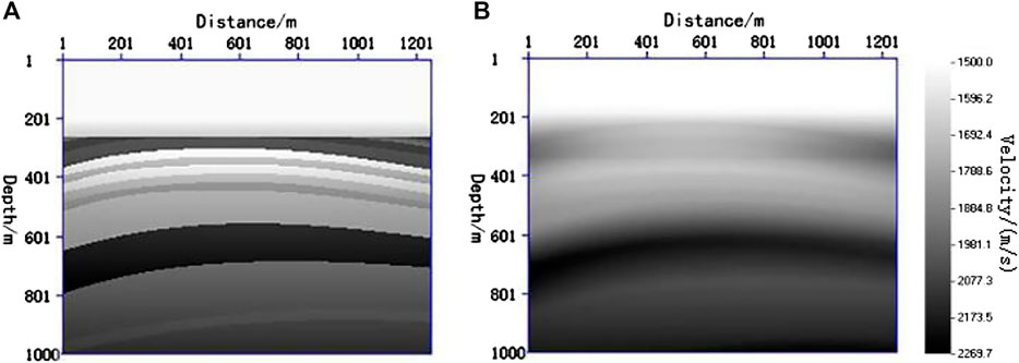
FIGURE 1. Velocity field of the simple model: (A) real velocity model; (B) Gaussian smooth velocity model.

It can be seen that conventional cross-correlation RTM results contain low-frequency noise (Figure 2A), coupled with strong near-surface energy caused by the source effect, resulting in unbalanced wave field energy, weak deep illumination, and unclear imaging. The LSRTM can solve the problems in RTM imaging. With an increase in the number of iterations, the data of Born forward simulation are gradually approaching the field data, and the migration profile is also gradually close to the reflection coefficient profile. As can be seen from the red arrows in Figures 2B,C, after 20 iterations, the noise in the shallow part of the migration profile gradually disappears, and the energy of the profile becomes more balanced, yielding clearer deep structure imaging. Under the same iteration times, the results of LSRTM processing by conjugate gradient normalization method are better than that by the conventional conjugate gradient method.

FIGURE 2

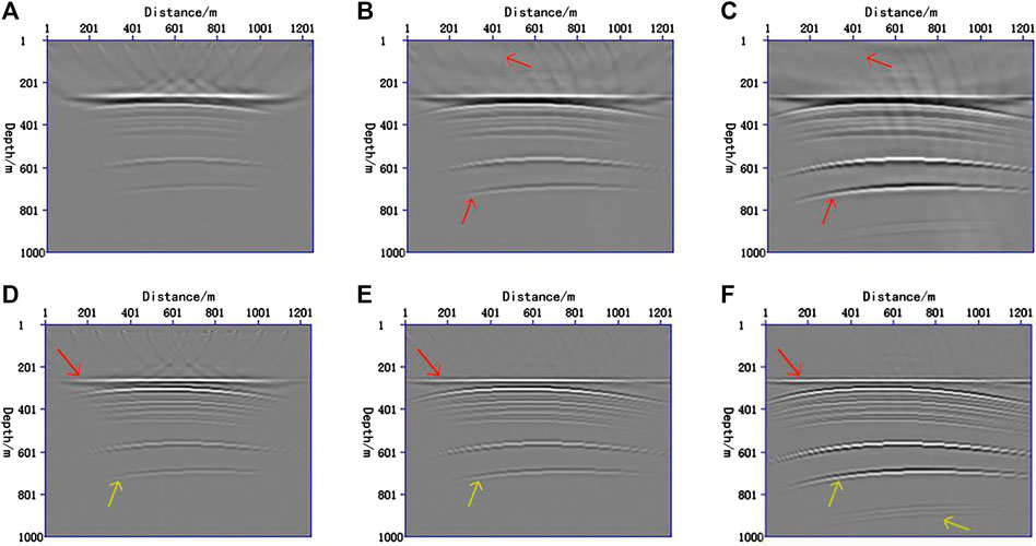
FIGURE 2. RTM and LSRTM migration profiles of a simple model. (A) cross-correlation RTM migration result; (B) result of cross-correlation conjugate gradient LSRTM with 20 iterations; (C) result of conjugate gradient normalized LSRTM with 20 iterations; (D) cross-correlation RTM following Laplace filtering; (E) cross-correlation conjugate gradient LSRTM following Laplace filtering; (F) conjugate gradient normalized LSRTM following Laplace filtering.

To eliminate low-frequency noise, Laplace filtering is performed on the profiles processed by RTM, cross-correlation conjugate gradient LSRTM, and conjugate gradient normalized LSRTM. From the comparison of red arrows in Figures 2D–F, it can also be seen that the amplitude of migration profile obtained by conjugate gradient LSRTM is more balanced than that obtained by RTM, and the imaging results of deep structure are better than that processed by RTM, while the migration profile obtained by conjugate gradient normalized LSRTM is better than that processed by the cross-correlation conjugate gradient LSRTM and RTM in both amplitude equalization and deep illumination (yellow arrow).

Complex model

To verify the applicability of the conjugate gradient normalized LSRTM for complex model, imaging experiments were carried out on the Marmousi model (Figure 3). The velocity model and the Gaussian smoothed velocity model are shown in Figures 3A,B. The lateral length of the model is 4,000 m and the depth is 2,495 m. It consisted of 650 traces with a trace interval of 5 m and 14 shots with a shot interval of 250 m. The receivers were fixed, and the shot point moved at equal intervals. The seismic records were obtained using finite-difference forward modeling (Figure 3C shows the single-shot record).

FIGURE 3

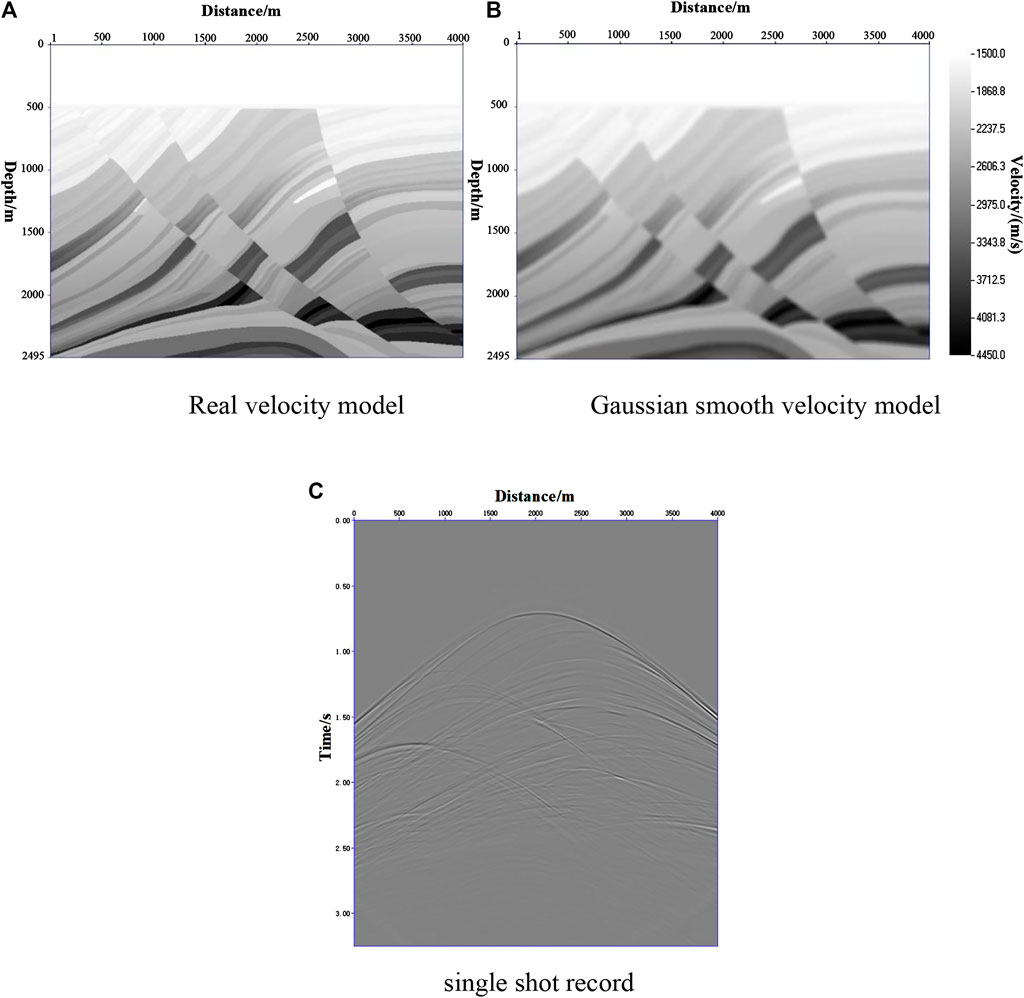
FIGURE 3. Velocity field and single-shot record of the Marmousi model. (A) real velocity model; (B) Gaussian smooth velocity model; (C) single-shot record.

The experimental work of the complex model was carried out on a workstation using the Intel(R) Xeon(R) Silver 4210R CPU @ 2.40 ghz, 128 GB memory, 64-bit operating system, and an X64-based processor. The graphics card was NVIDIA GeForce RTX3090 with 24 GB of video memory. In this computing environment, both the conventional LSRTM and conjugate gradient normalized LSRTM take approximately 3 min per iteration.

The real and Gaussian smoothed velocity field of Marmousi are shown in Figures 4A,B, which is used for the background velocity field of the RTM and LSRTM migration. From the migration results shown in Figures 4A,B, both cross-correlation RTM and normalized cross-correlation RTM will be contaminated by low-frequency noise (indicated by the yellow arrow). The low-frequency noise in the shallow part of the cross-correlation RTM is more serious. Normalized cross-correlation RTM is better in suppressing the noise in the shallow part, but there will be a small amount of low-frequency noise in the deep part. The main reason for this is that although the source-normalized imaging conditions suppress the shallow strong energy and enhance the deep illumination, they also enhance the wave field energy in the continuation process. The LSRTM can eliminate the low-frequency noise very well. It can be seen from Figures 4C,D (yellow arrow) that the low-frequency noise in the shallow part is obviously eliminated by least-squares processing, and as the number of iterations increases, the noise will continue to weaken. By comparing the low-frequency noise suppression results of the two imaging conditions, under the same number of iterations, the conjugate gradient normalized LSRTM is more significant for low-frequency suppression. In contrast, strong shallow low-frequency noise affects the imaging of underground structures by RTM. Figures 4E,F (red arrow) clearly show that reverse-time migration under different imaging conditions does not achieve accurate imaging of underground structures, some events cannot reflect accurate structure information well, and there are residual low-frequency noises in shallow parts. After the LSRTM processing, it can be seen from Figures 4G,H (red arrows) that the LSRTM can well eliminate low-frequency noise and realize accurate imaging of underground structures, and the overall amplitude of the profile is more balanced. Compare the underground illumination of the LSRTM under two different imaging conditions, it can be seen from the two enlarged images Figures 4I,J (corresponding to the two red dashed rectangular boxes in Figures 4G,H), the conjugate gradient normalized LSRTM is significantly stronger for the deep illumination than the result of the cross-correlation LSRTM. From the comparison of the whole section, we can also see that the conjugate gradient normalized LSRTM is better than the conventional LSRTM for noise suppression in the shallow part, illumination of the deep part, and imaging of the whole structure.

FIGURE 4

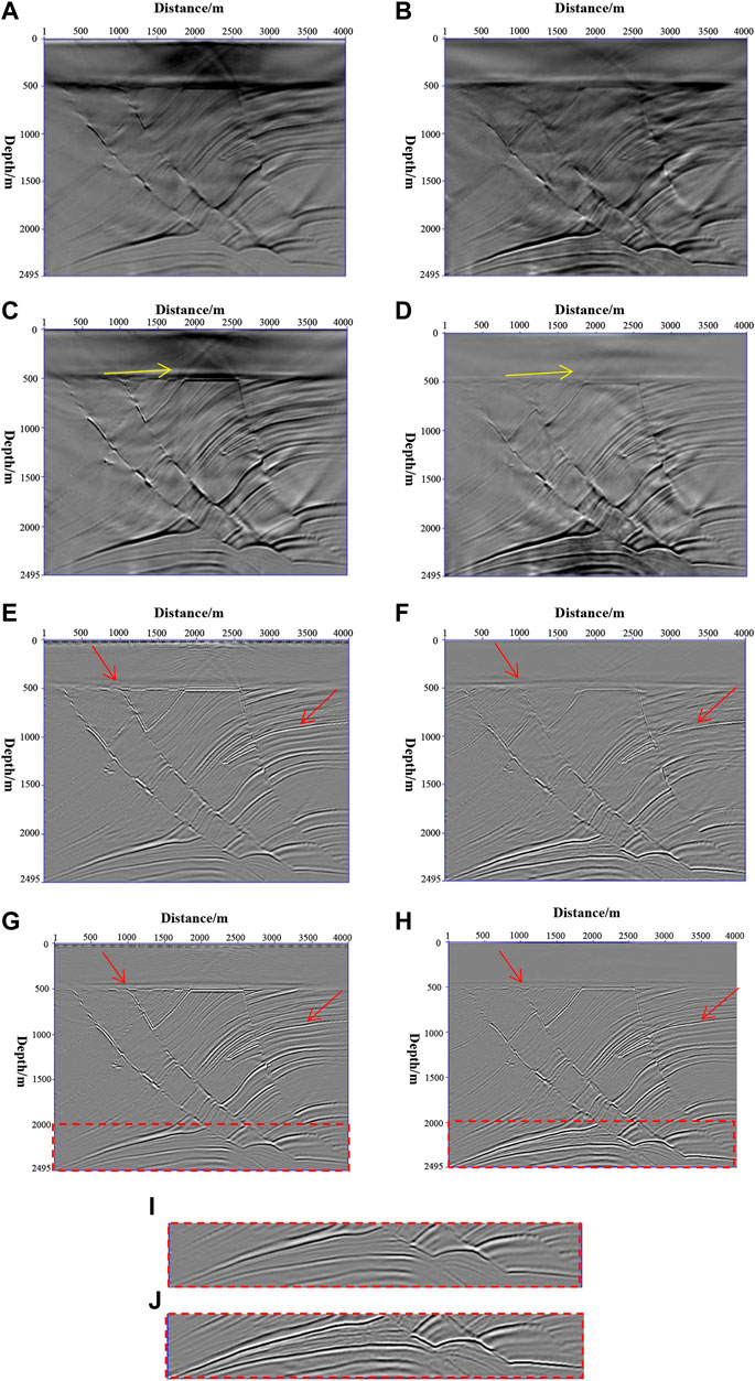
FIGURE 4. RTM and LSRTM of the Marmousi model. (A) RTM migration results; (B) normalized cross-correlation RTM migration results; (C) results of cross-correlation conjugate gradient LSRTM with 15 iterations; (D) results of conjugate gradient normalized LSRTM with 15 iterations; (E) Laplace filtering results of Figure 4 (A); (F) Laplace filtering results of Figure 4 (B); (G) Laplace filtering results of Figure 4 (C); (H) Laplace filtering results of Figure 4 (D); (I,J) are partial enlarged views of the red rectangular boxes in Figure 4 (G,H), respectively.

The spectrum of Figure 4G is shown in Figure 5A, and the spectrum of Figure 4H is shown in Figure 5B. Comparing Figures 5A,B, it can be seen that the conjugate gradient normalized LSRTM has a wider frequency band and more information. This also shows the superiority of conjugate gradient normalized LSRTM in the spectrum.

FIGURE 5

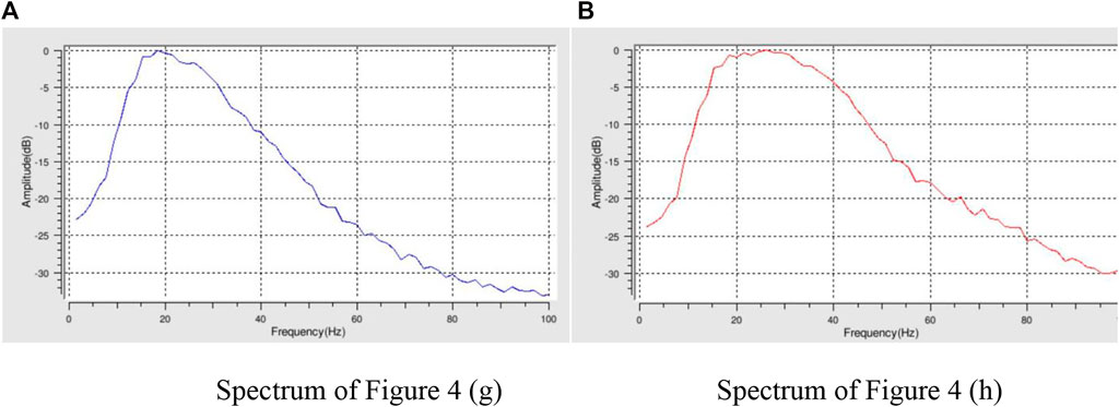
FIGURE 5. Spectrum of LSRTM. (A) spectrum of Figure 4 (g). (B) spectrum of Figure 4 (h).

Imaging efficiency comparison

To compare the convergence speed of conjugate gradient normalized LSRTM and conventional conjugate gradient cross-correlation LSRTM, Figure 6 shows the comparison between the seismic records of Born approximate simulation and the observation records under the same number of iterations for the same shot in the simple model.

FIGURE 6

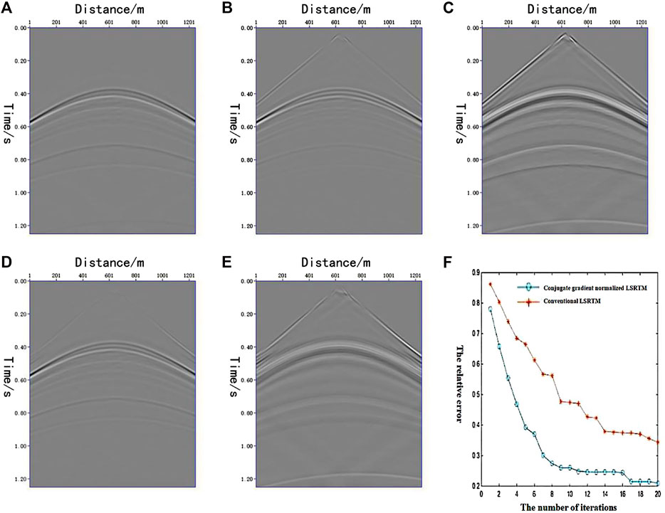
FIGURE 6. Seismic record and error curve of simple model. (A) the 6th observation seismic record; (B) the 6th simulation record of Born approximate forward modeling after 20 iterations by the conventional conjugate gradient cross-correlation LSRTM; (C) the difference between (A,B); (D) the 6th simulation record of Born approximate forward modeling after 20 iterations by conjugate gradient normalized LSRTM; (E) the difference between (A,D); (F) the normalized error reduction curve of the observation record and the simulation record.

Figure 6A shows the sixth observation seismic record. The sixth shot simulation records of Born approximate forward modeling after 20 iterations of conventional conjugate gradient cross-correlation LSRTM, and conjugate gradient normalized LSRTM are shown in Figures 6B,D. We calculated the difference between the simulation record and observation record of the two LSRTM methods (Figures 6C,E). From the comparison of Figures 6C,E, it can be seen that under the same number of iterations, the Born approximate forward modeling record using the conjugate gradient normalized LSRTM is closer to the observation.

The normalized error reduction curve of the observation record and the simulation is shown in Figure 6F. The abscissa is the number of iterations of the two LSRTM methods, and the ordinate is the relative error. The error formula can be expressed as

${\mathit{E}}_{\mathit{r}}=\frac{\left|{\mathit{R}}_{\mathit{o}}-{\mathit{R}}_{\mathit{s}}\right|}{{\mathit{R}}_{\mathit{o}}},(24)$

where E_r is the relative error, R_o denotes the observation record, and R_s denotes the simulation record. Figure 6F shows that compared to the conventional LSRTM, the conjugate gradient normalized LSRTM converges faster, and the residual error will eventually converge to a lower level. Therefore, it can be seen from the above results that the conjugate gradient normalized LSRTM converges faster than the conventional LSRTM, and its residual error is smaller after 20 iterations.

Trial processing of field data

To test the adaptability of the method to the field data, two-dimensional land-based real data were imaged using the conjugate gradient normalized LSRTM. The velocity model of the field data and single-shot record are presented in Figures 7A,B. The velocity field of these data has a horizontal length of 32,050 m and a depth of 7,560 m. The data consisted of 328 shots with the shot interval of 100 m. The time sampling was 6 s with the sampling rate at 4 ms. Figure 8A shows the result of conventional normalized cross-correlation RTM filtering of field data, and Figure 8B shows the result of 20 iterations of conjugate gradient normalized LSRTM filtering. The conjugate gradient normalized LSRTM is superior to the conventional normalized cross-correlation RTM method, in both the suppression of shallow low-frequency noise and the illumination of deep structures. The energy of the shallow and deep layers of the method in this study is more balanced, and the profile imaging is better, especially for the middle and shallow imaging (as shown in the red box). Thus, it is better than the conventional normalized cross-correlation RTM method.

FIGURE 7

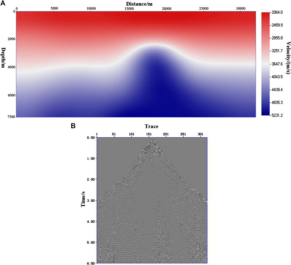
FIGURE 7. Velocity field of field seismic data and single-shot record.

FIGURE 8

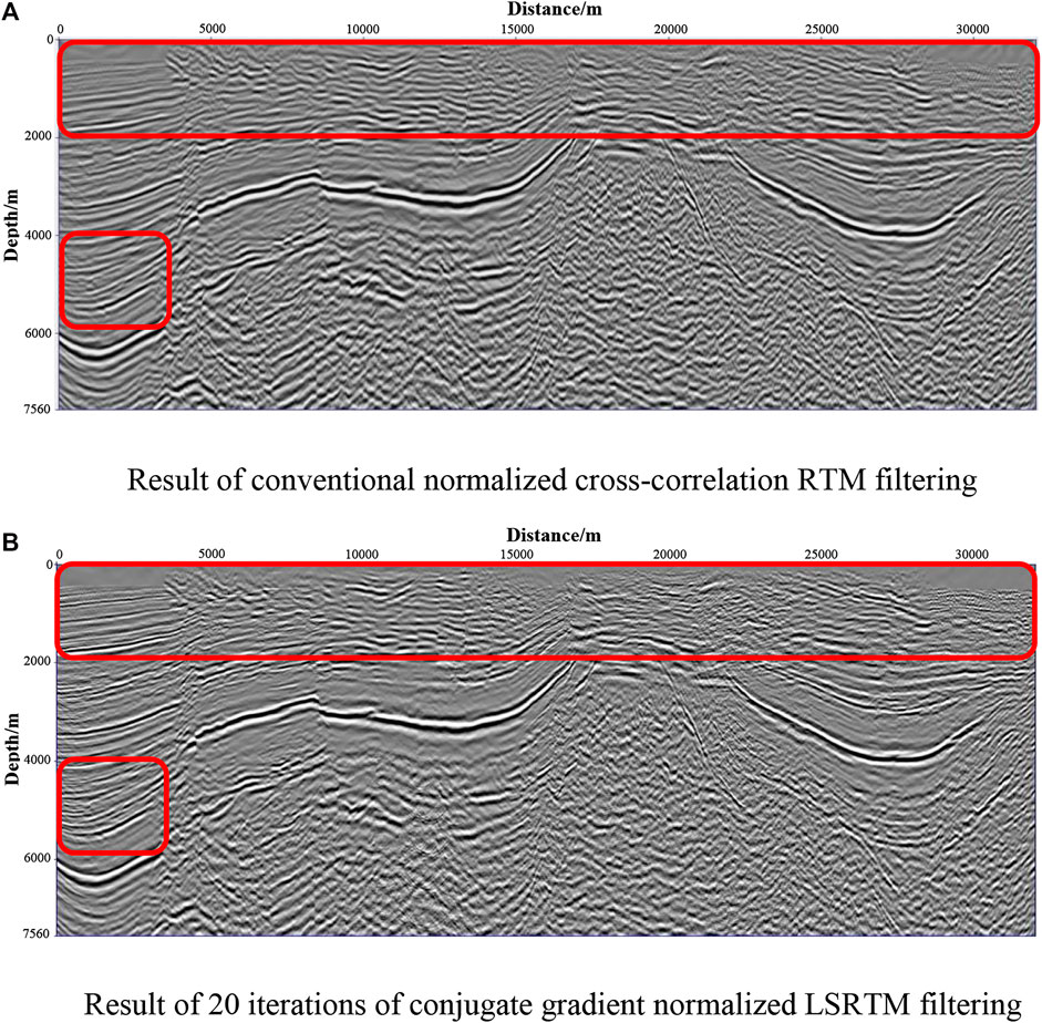
FIGURE 8. Comparison of imaging results by different methods. (A) results of conventional normalized cross-correlation RTM filtering; (B) results of 20 iterations of conjugate gradient normalized LSRTM filtering.

Conclusion and discussion

This study proposed an effective LSRTM method using the source-normalized steepest descent gradient. Examples of the model and field data were carried out, and the main conclusions are as follows:

1) Compared with the conventional conjugate gradient LSRTM, the normalized LSRTM can help to reduce shallow low-frequency noise, enhance underground deep illumination, and weaken the source effect, which thus improves the imaging quality of underground structures.

2) Under the same number of iterations, the Born approximation forward record of the gradient normalized LSRTM method is closer to the observation record than the conventional LSRTM method. The convergence speed of the gradient normalized LSRTM is faster, and its residual error eventually converges to a lower level.

3) In the present work, only P-waves were considered. The application of converted waves will be studied in the future (Nemeth et al., 1999; Kuehl and Scachi, 2001b; Huang et al., 2013b; Yang et al., 2018).

Data availability statement

The raw data supporting the conclusions of this article will be made available by the authors, without undue reservation.

Author contributions

All authors contributed to design of the study. YS and LT debugged the programs of RTM conventional LSRTM and conjugate gradient normalized LSRTM. XX analyzed the characteristics of the simulation data and field data. YS and XX wrote the first draft of the manuscript. All authors contributed to manuscript revision, read, and approved the submitted version.

Funding

The study is supported by the National Key R&D Program of the Ministry of Science and Technology of China (Intergovernmental Cooperation on Scientific and Technological Innovation, 2021YFE0108800) and the Open Fund Project of National Engineering Laboratory for Offshore Oil Exploration (CCL2020RCPS0419RQN).

Acknowledgments

The authors would like to thank the Shengli Geophysical Research Institute of Sinopec for providing the field data. They also thank the reviewers for their constructive comments and suggestions, which significantly improved the quality of this article.

Conflict of interest

The authors declare that the research was conducted in the absence of any commercial or financial relationships that could be construed as a potential conflict of interest.

Publisher’s note

All claims expressed in this article are solely those of the authors and do not necessarily represent those of their affiliated organizations, or those of the publisher, the editors, and the reviewers. Any product that may be evaluated in this article, or claim that may be made by its manufacturer, is not guaranteed or endorsed by the publisher.

References

Bamberger, A., Chavent, G., Hemon, C., and Lailly, P. (1982). Inversion of normal incidence seismograms. Geophysics 47 (5), 757–770. doi:10.1190/1.1441345

CrossRef Full Text | Google Scholar

Aoki, N., and Schuster, G. T. (2009). Fast least-squares migration with a deblurring filter. Geophysics 74 (6), WCA83–WCA93. doi:10.1190/1.3155162

CrossRef Full Text | Google Scholar

Baysal, E., Kosloff, D. D., and Sherwood, J. W. C. (1983). Reverse time migration. Geophysics 48 (11), 1514–1524. doi:10.1190/1.1441434

CrossRef Full Text | Google Scholar

Claerbout, J. F. (1992). Earth soundings analysis: Processing versus inversion. Boston: Blackwell Scientific Publications.

Google Scholar

Guo, S. J., Ma, F. Z., Duan, X. B., and Wang, L. (2015). Research of least-squares reverse-time migration migration imaging method and its application. Geophys. Prospect. Petroleum 54 (3), 301–308. doi:10.3969/j.issn.1000-1441.2015.03.008

CrossRef Full Text | Google Scholar

Herrmann, F. J., Brown, C. R., Erlangga, Y. A., and Moghaddam, P. P. (2009). Curvelet-based migration preconditioning and scaling. Geophysics 74 (4), A41–A46. doi:10.1190/1.3124753

CrossRef Full Text | Google Scholar

Huang, J. P., Li, Z. C., Liu, Y. J., Kong, X., Cao, X., and Xue, Z. (2013a). The least square pre-stack depth migration on complex media. Prog. Geophys 28 (06), 2977–2983. doi:10.6038/pg20130619

CrossRef Full Text | Google Scholar

Huang, J. P., Li, Z. C., Kong, X., Liu, Y., Cao, X. L., and Xue, Z. (2013b). A study on least-squares migration imaging method for fractured-type carbonate reservoir. Chin. J. Geophys 56 (5), 1716–1725. doi:10.6038/cjg20130529

CrossRef Full Text | Google Scholar

Huang, J. P., Li, C., Li, Q. Y., Guo, S. J., Duan, X. B., Li, J. G., et al. (2015). Least-squares reverse time migration with static plane-wave encoding. Chin. J. Geophys 58 (06), 2046–2056. doi:10.6038/cjg20150619

CrossRef Full Text | Google Scholar

Huang, J. P., Li, C., and Li, Q. Y. (2016). Theory and method of least squares migration imaging. Beijing: Science Press.

Google Scholar

Kuehl, H., and Scachi, M. D. (2001a). “Split step WKBJ least squares migration/inversion of incomplete,” in Expanded abstracts of 5th SEGJ international symposium imaging technology, 200–204.

Google Scholar

Kuehl, H., and Sacchi, M. D. (2001b). Generalized least‐squares DSR migration using a common angle imaging condition. Seg. Tech. Program Expand. Abstr. 20 (1), 1025. doi:10.1190/1.1816254

CrossRef Full Text | Google Scholar

Kuehl, H., and Sacchi, M. D. (2003). Least‐squares wave‐equation migration for AVP/AVA inversion. Geophysics 68 (1), 262–273. doi:10.1190/1.1543212

CrossRef Full Text | Google Scholar

Liu, X. W. (2008). Fundamentals of elastic wave field theory. Qingdao: Ocean University of China, 147–150.

Google Scholar

Nemeth, T., Wu, C., and Schuster, G. T. (1999). Least‐squares migration of incomplete reflection data. Geophysics 64 (1), 208–221. doi:10.1190/1.1444517

CrossRef Full Text | Google Scholar

Prucha, M. L., and Biondi, B. L. (2002). Subsalt event regularization with steering filters. in SEG technical program expanded abstracts 2002 (Society of Exploration Geophysicists), 1–17.

CrossRef Full Text | Google Scholar

Tarantola, A. (1984). Inversion of seismic reflection data in the acoustic approximation. Geophysics 49, 1259–1266. doi:10.1190/1.1441754

CrossRef Full Text | Google Scholar

Wang, J., Kuehl, H., and Sacchi, M. D. (2003). Least‐squares wave‐equation AVP imaging of 3D common azimuth data. Seg. Tech. Program Expand. Abstr. 22 (1), 1039. doi:10.1190/1.1817449

CrossRef Full Text | Google Scholar

Wang, Y. F., Yang, C. C., and Duan, Q. L. (2009). On iterative regularization methods for migration deconvolution and inversion in seismic imaging. Chin. J. Geophys 52 (06), 1615–1624. (in Chinese). doi:10.1002/cjg2.1392

CrossRef Full Text | Google Scholar

Yang, H., Liu, W., Xu, F., and Wang, F. (2018). “Reverse time migration with combined source-receiver illumination,” in SEG technical program expanded abstracts, 4448–4452. doi:10.1190/segam2018-2997690.1

CrossRef Full Text | Google Scholar

Yang, Q. Q., and Zhang, S. L. (2008). Least-squares Fourier finite-difference migration. Prog. Geophys. 23 (02), 433–437.

Google Scholar

Yao, G., and Wu, D. (2015). Least-squares reverse-time migration for reflectivity imaging. Sci. China Earth Sci. 58, 1982–1992. doi:10.1007/s11430-015-5143-1

CrossRef Full Text | Google Scholar

Zhang, Y., Duan, L., and Xie, Y. (2015). A stable and practical implementation of least-squares reverse time migration. Geophysics 80, V23–V31. doi:10.1190/geo2013-0461.1

CrossRef Full Text | Google Scholar