Estimating the Actual Evapotranspiration of Different Vegetation Types Based on Root Distribution Functions

Background and Aims: Evapotranspiration is an important part of the water cycle and energy cycle. However, even under the same climatic condition, there are spatial differences in actual evapotranspiration (ET_a) due to different land use and land cover. To characterize the influence of different vegetation types on ET_a in China, this study parameterized the vertical distribution of the root systems of different vegetation types.

Methods: A one-dimensional soil-plant-atmosphere continuum (SPAC) model was constructed, and these root distribution functions were used to improve the root water absorption modulus of the soil-plant-atmosphere continuum model. Based on the improved model, the actual evaporation actual transpiration and ET_a under different vegetation types were calculated, and the reasons for different ET_a of different vegetation types were analyzed.

Results: The results show that the root distribution of all vegetation types increases first and then decreases as the depth increases, and almost all the maximum values are in the range of 0–20 cm. The savanna has the shallowest root system, while the barren has the deepest root system. The average ET_a calculated in China was about 342.2 mm/y in 2015. The average ET_a of the broadleaf evergreen forests is the largest, about 773 mm/y and the barren is the smallest, about 151 mm/y. The average annual precipitation is the most important factor affecting the ET_a differences of different vegetation types.

Conclusion: The results provide solutions for estimating the ET_a of different vegetation types and are significant to water resources management and soil and water conservation.

1 Introduction

Evapotranspiration (ET) is an integral part of the hydrological cycle and the second most significant part of the water cycle in most terrestrial areas (after precipitation) (Allen et al., 1998; Liu et al., 2010). To correctly manage and allocate water resources, it is necessary to accurately assess ET under different climates, geographic regions and land use, espically actual evapotranspiration (ET_a) (Peters et al., 2011). However, the ET_a under different vegetation types is still challenging to distinguish quantitatively. Accurately distinguishing the ET_a under different vegetation types contributes to the rational allocation of water resources in different ecosystems and has an important guiding significance for agricultural water-efficient irrigation, combating desertification, and soil and water conservation (Li et al., 2017; Du et al., 2019; Sun et al., 2020). It is also crucial for the quantitative assessment of the hydrological cycles and climate change in different regions. For terrestrial ecological hydrology, climate change, and other models, estimating root water uptake is the key factor in quantifying vegetation transpiration, and the difference in root distribution is critical in distinguishing between the water uptake of different vegetation roots (Zeng et al., 1998; Zeng, 2001; Kumar et al., 2015).

When calculating the ET_a under different vegetation types, if the water uptake by plants in several soil layers is considered, the vertical distribution of the roots can represent the water uptake rate of the plant’s roots in different soil layers (Zeng, 2001). The ET_a of different vegetation types can be obtained by simulating the vertical distribution of different vegetation root systems. Therefore, in the relevant models of plant water absorption, the parameterization of root distribution is very important. However, as the root system grows in the soil, it is not easy to sample in a large area. Researchers often use different root distribution models for different land surface models, due to the lack of root distribution data to parameterize a global root distribution function (Nepstad et al., 1994; Jackson et al., 1996; Zeng, 2001).

The collection of a large amount of root data is a key to rebuild the root distribution of plants over a wide range. Some researchers supplement the parameterization of root distribution by collecting root distribution data from existing data. For example, Gale and Grigal (1987) summarized 123 root distribution data from 19 articles and fitted a single factor root distribution function. Jackson et al. (1997) and Canadell et al. (1996) integrated root data from over 200 documents worldwide. They built a comprehensive and significant database on maximum root depth, root distribution, biomass and other data of terrestrial biological communities. The root distribution parameters of 11 major terrestrial biological communities are obtained through single factor function fitting, which is widely used. Based on the database, Zeng (2001) improved the single factor root distribution function by considering the maximum root depth and obtained the two-factor root distribution function, which applies to the three most widely used land cover types with three sets of parameters. These root distribution data were used in the European Centre for Medium-Range Weather Forecasts (ECMWF) operational model and global reanalysis (Zeng, 2001). Schenk and Jackson (2002a) proposed a logistic dose-response curve (LDR), which collected 475 root profiles and fitted the root distribution parameters of 15 types of plants worldwide.

However, these global studies are extensive in scope, and the simulation of root distribution on a small scale is not accurate enough. More concentrated collection of target areas or target vegetation types is required. To obtain more precise vegetation root distribution parameters, some researchers collect and analyze data on the vegetation root of a specific type of vegetation or a particular area. For example, Fan et al. (2016) collected the root distribution data from temperate crops and used the LDR function to adjust them to obtain the root distribution parameters of 14 temperate crops. Yang et al. (2009) collected plant root samples from the Qinghai-Tibet Plateau and used a single factor function adjustment to obtain the parameter β (i.e., the parameter of the single factor function) of three alpine vegetation. The root distribution data of the area can be collected and parameterized to obtain the more accurate root distribution parameters with regional characteristics or vegetation characteristics, thus improving the accuracy of the eco-hydrological process simulation in the area. However, the study focused on the distribution of vegetation roots in the scale of the whole China is few. Furthermore, the three global root distribution models fit with limited data from China (Jackson et al., 1996; Zeng, 2001; Schenk and Jackson, 2002a). These models’ parameters are insufficient to replace the root distribution of Chinese vegetation. Therefore, China was selected as the study area.

Soil-plant-atmosphere continuum (SPAC) theory is a primary system theory in the field of ET evaluation. The SPAC system effectively integrates soil, plant and atmospheric systems. It suggests using a “water potential” energy unit to quantitatively study the energy change of water in each link to calculate water flux (Philip, 1966). A SPAC model based on this system can consider the effects of soil moisture and different vegetation cover types on ET. In the root water uptake module of the SPAC model, different root distribution functions can be used according to different vegetation types to distinguish the root water uptake of different vegetation types and then combined with the soil water stress function to obtain ET_a. In the SPAC model, the actual evaporation can also be calculated based on the topsoil evaporation module. Therefore, this study uses a one-dimensional SPAC model to estimate the ET_a under different vegetation coverage. Since the availability of meteorological date such as precipitation and temperature in 2015 is accessible, the ET_a in 2015 was calculated to analyze the impact of root distribution parameters of different vegetation on ET_a.

In summary, China was selected as the study area and 2015 was selected as the simulation period. There are two main goals: 1) to parameterize the vertical root distribution of different vegetation types in China’s terrestrial areas and obtain parameters that can more accurately simulate the vertical distribution of vegetation roots in China; 2) apply the root system distribution function to the one-dimensional SPAC model to explore the impact of different vegetation types in China on ET_a. In this study, a database of vegetation root distribution in China was constructed, and vertical root distribution parameters with characteristics of Chinese vegetation were obtained, which provides a theoretical basis for simulating ecological processes, hydrological processes and climate simulation of different vegetation coverage types in China. This study is an essential practical guide for agricultural water-efficient irrigation, soil and water conservation, desertification control, etc.

2 Materials and Methods

2.1 Root Data Sources

Based on the core collection of Web of Science (WoS) and China National Knowledge Infrastructure (CNKI), the research collected 277 articles related to the distribution of plant roots, including the vertical distribution data of plant roots at 281 research sites and 786 sections (Figure 1, references from Appendix). Among them, 20 (2.5%) sections are divided into two layers, 103 (13.1%) sections are divided into three layers, and 663 (84.4%) sections are divided into more than four layers. Among all sections, the maximum depth of 576 sections (73.3%) is less than 100 cm, and the maximum depth of 167 sections (21.2%) is between 100 and 200 cm. In addition to collecting and sorting out the root distribution data of each profile, this study also recorded other detailed information such as the geographic location (longitude, latitude, altitude), soil type, annual precipitation, annual average temperature, root measurement type (total, fine and thick), measurement methods, measurement items (root biomass, root length, root length density, etc.), sampling depth and others for each sample point. Because of the different measurement items of root distribution, this study will uniformly convert them into a proportional form to compare and analyze them.

FIGURE 1

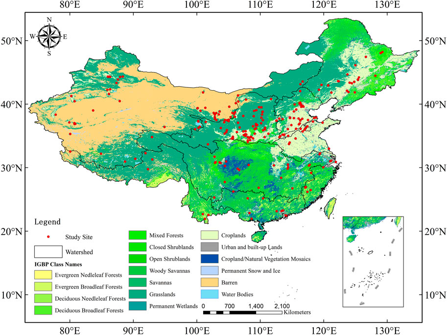
FIGURE 1. Land cover map (IGBP) and geographic locations of root profiles in the China database. Data from Appendix.

The classification of vegetation types adopts the International Geosphere-Biosphere Program (IGBP) (Sweeney, 1997; Zeng, 2001; Friedl et al., 2010). This program divides all land cover types into 17 categories, including 12 types of natural vegetation (including wasteland) and five types of no vegetation cover. In this study, a land cover type map was drawn based on Moderate Resolution Imaging Spectroradiometer (MODIS) remote sensing data products (Figure 1). All root profiles collected were classified according to the IGBP classification scheme. Classification results are evergreen needleleaf forests (n = 43), evergreen broadleaf forests (n = 46), deciduous needleleaf forests (n = 1), deciduous broadleaf forests (n = 176), mixed forests (n = 2), closed shrublands (n = 33), open shrublands (n = 63), woody savannas (n = 1), savannas (n = 10), grasslands (n = 54), croplands (n = 315) and barren (n = 41). It should be noted that, although parameters of these vegetation types have been optimized in this study, the ET_a of deciduous needleleaf forests, mixed forests, and woody savannas were not analyzed statistically due to the small number of samples (n < 3).

2.2 Root Vertical Distribution Model and Parameter Optimization Method

In this study, three cumulative root distribution functions were selected for parameter optimization, i.e., finding the optimal parameters of the root distribution function within a given range based on the measured data. These three functions are all fitted from global root distribution data and consider several types of vegetation (Jackson et al., 1996; Schenk and Jackson, 2002a; Zeng, 2001). The cumulative distribution functions of the three root systems are shown in Eqs 1–3. Eq. 1 is a single factor function of the vertical distribution of root systems of major terrestrial communities in the world (Gale and Grigal, 1987). This equation has simple parameters and wide applications and is widely cited (Jackson et al., 1996). Zeng (2001) developed Eq. 2 using the single factor function (Jackson et al., 1996), considering the depth of the root and refined it to obtain a two-factor function. This equation and associated parameters were used in the open ECMWF model and the global reanalysis dataset. Eq. 3 is the LDR curve proposed by Schenk and Jackson (2002a), based on the relationship between root system depth and root system distribution.

$Y=1-{\beta }^d(1)$

$Y=1-\frac{1}{2}\ast \left(e^{-a\ast D}+e^{-b\ast D}\right)(2)$

$r\left(\text{d}\right)=\frac{R_{max}}{1+{\left(\frac{d}{D_{50}}\right)}^c} (3)$

In the equation, Y is the cumulative root distribution ratio of the soil surface to the depth d (cm), the range is [0,1]; β is a single parameter with no physical significance; a and b are typical plant-related parameters, and the unit is m^{− 1}; D refers to the soil depth, in m; r(d) refers to the cumulative root number (or biomass, length) above the profile depth d, corresponding to the $R_{max}$ unit; $R_{max}$ refers to the total root number in the profile (or total biomass, total Length); $D_{50}$ refers to the depth when r(d) = 0.5 $R_{max}$, in cm; c refers to a dimensionless parameter, which is only related to plant types.

Since Eq. 3 describes the cumulative distribution function of the root system, the unit of r(d) in the equation will with the change in $R_{max}$. To unify the units of each function and make it easier to calculate the root distribution ratio of each layer of the plant, Eq. 3 is converted into a root cumulative distribution function, as shown in Eq. 4:

$Y=\frac{1}{1+{\left(\frac{d}{D_{50}}\right)}^c} (4)$

In Eq. 4, Y is the cumulative proportion of the root system, and the range is [0,1]; $D_{50}$ is the root system depth when Y = 0.5, in cm; the other parameters are the same as in Eq. 3.

Root Mean Square Error (RMSE) ranged from 0 to 1 was chosen as a quantitative index (Kennedy and Neville, 1986), which is given by:

$RMSE=\sqrt{\frac{{\displaystyle \sum {\left(P_i-O_i\right)}^2}}{n}}(5)$

In Eq. 5, $O_i$ and $P_i$ represent the proportion of observed and predicted roots in layer i, and n is the number of root layers. The optimization ranges of the parameters of the single factor function (Eq. 1) are fixed at [0.9,1] (Jackson et al., 1996). The range of the four parameters (a, b, $D_{50}$, c) in the two-factor function (Eq. 2) and LDR curve (Eq. 4) is defined between the maximum and minimum values, that is, the ranges of a, b, $D_{50}$, and c are 4.372 to 10.74, 0.978 to 2.614, 5 to 28, and -2.621 to -1.176, respectively (Zeng, 2001; Schenk and Jackson, 2002a).

In this study, each vegetation type will be fitted according to three root distribution models, and the three mean RMSE will be calculated according to the three fitting results. The root distribution model with the smallest mean RMSE was selected for each vegetation type.

2.3 Construction of One-Dimensional SPAC Model and Calculation of ET

A one-dimensional SPAC model was constructed in this study, including a soil infiltration module, a soil water movement module, a topsoil evaporation module, and a root water absorption module. The model’s basic assumption is that the water in the cell mainly moves vertically, and the water movement in the horizontal direction is ignored. The SPAC model concept diagram was shown in Figure 2.

FIGURE 2

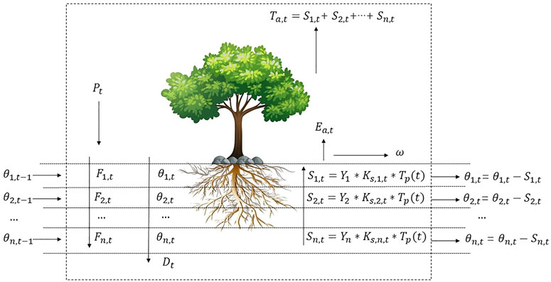
FIGURE 2. One-dimensional Soil Plant Atmosphere Continuum model concept diagram. $P_t$ is daily precipitation at the current time step. $T_{a,t}$ is daily actual transpiration at the current time step, which is the sum of root water uptake volume. $E_{a,t}$ is daily actual evaporation at the current time step. ${\theta }_{n,t-1}$ is soil moisture of nth layer before the current time step. $F_{n,t}$ is the infiltration volume of the nth layer at the current time step. $S_{n,t}$ is the root water uptake volume of the nth layer at the current time step. $Y_n$ is the root percent of the nth layer in this pixel. $K_{s,n,t}$ is the response coefficient of water stress in the nth layer at the current time step. $\omega$ is the amount of uninfiltrated water at the end of the current time step.

2.3.1 Soil Infiltration Module

The soil infiltration module adopts the Green-Ampt layered infiltration model modified by Fleechinger (2000) to calculate the cumulative infiltration amount in each layer:

$F_{\ast }=\frac{1}{2}\ast \left(t_{\ast }-2z_{\ast }+\sqrt{{\left(t_{\ast }-2z_{\ast }\right)}^2-8t_{\ast }}\right)(6)$

where $F_{\ast }$ is the dimensionless cumulative infiltration volume; $t_{\ast }$ is the dimensionless time; $z_{\ast }$ is the dimensionless depth.

2.3.2 Soil Moisture Movement Module

The soil water movement module uses the one-dimensional Richards equation, combined with the Van Genuchten model, to numerically simulate the soil water movement (Richards, 1931; Van Genuchten, 1980), which is given by:

$C\left(\psi \right)\frac{\partial \psi }{\partial \text{t}}=\frac{\partial }{\partial z}\left[K\left(\psi \right)\frac{\partial \psi }{\partial z}\right]-\frac{\partial K\left(\psi \right)}{\partial z}(7)$

where C is the specific water capacity; ψ is the soil matrix potential; is the soil moisture content, m³/m³; K is the soil unsaturated hydraulic conductivity, m³/d; t is the time, day; z is the vertical coordinate, down is positive.

2.3.3 Topsoil Evaporation Module

The evaporation modulus of the topsoil uses the empirical function proposed by Belmans et al. (1983). According to the extinction coefficient and leaf area index (LAI), the ET_p is divided into potential transpiration (T_p) and potential evaporation (E_p).

$E_P=E{T}_P\text{∗}{e}^{-kgr\ast LAI}(8)$

$T_P=E{T}_P-E_P(9)$

The actual surface evaporation (E_a) is calculated as follow:

$E_a=E_P\ast K_s(10)$

In Eqs 8–10, $E_P$ , $E_a$ , and $E{T}_P$ in mm/day; $K_s$ is the water stress coefficient (see section 2.3.4); $kgr$ is the reduction coefficient, set at 0.6 in this study.

2.3.4 Root Water Absorption Module

The root water absorption module calculates the layered stress of T_p to obtain the actual water absorption (i.e., T_a) of plant roots. This module is modified based on the Feddes model (Feddes and Zaradny, 1978). Considering the influence of soil moisture, root distribution functions of different vegetation can also be used to distinguish their root water absorption. For example, after determining that the vegetation coverage type is an evergreen coniferous forest, the corresponding root system distribution function and parameters can be obtained according to the root vertical distribution model and parameter optimization method. These root distribution functions and their parameters are used to calculate root water absorption. Finally, the ET of evergreen coniferous forest vegetation can be obtained. The modified equation is as follows:

$S\left(z,t\right)=K_s\ast Y\left[z\right]\ast T_p\left(t\right)(11)$

In Eq. 11, S(z, t) refers to the root water absorption in mm; $K_s$ is the response function of water stress; $Y\left[z\right]$ is the root density distribution function, which is replaced by Eqs 1–3. Different formulas are used for land cover types. See Supplementary Table S1 for details; $T_p$ in mm.

The water stress response function is a key function of soil moisture affecting ET_a, which is very important throughout the model. This study uses the water stress response function proposed in the FAO-56 (Allen et al., 1998). The equation is as follows:

$K_s=\frac{TAW-D_r}{TAW-RAW}=\frac{TAW-D_r}{\left(1-p\right)\ast TAW}(12)$

$TAW = 1000\ast \left({\theta }_{FC}-{\theta }_{WP}\right)\ast zr(13)$

$RAW=p\ast TAW(14)$

$D_{r,i-1}=1000\ast \left({\theta }_{FC}-{\theta }_{i-1}\right)\ast zr(15)$

In Eqs 12–15, $K_s$ refers to the coefficient of water stress, in the range [0,1]; TAW refers to the total available soil moisture in the root zone in mm; RAW refers to the soil moisture available in the root zone in mm; $D_r$ refers to the water consumption in the root zone, $D_{r,i-1}$ refers to the root water consumption of the i-1 layer in mm; p refers to the proportion of TAW that the crop can be extracted from the roots without being exposed to water stress, the fixed value is 0.5 in this model; ${\theta }_{WP}$ refers to the wilting point in m³/m³. In this study, the residual moisture content ${\theta }_r$ is used instead; ${\theta }_{FC}$ refers to the field water holding capacity in m³/m³; ${\theta }_{i-1}$ refers to the soil moisture content of the i-1 layer in m³/m³; zr is the root depth in m.

2.3.5 Boundary Conditions and Initial Conditions Setting

The upper boundary is defined as a free boundary, including ET, precipitation, and so on. The lower boundary condition is set as a free drainage state. The model simulation time step is 1 day, the simulation continues for 365 days, the only moisture source is precipitation, and the unit is mm/day. The soil layer selected in the model is 0–200 cm, divided into 20 layers; each layer is 10 cm. The initial soil water potential is set to -0.5 to -1.95 m with an interval of 0.1 m. Depending on the growing conditions of the plants, plants only have transpiration when the temperature is 10°C or above, and there is no transpiration when the temperature is less than 10°C.

2.3.6 Calculation of ET_a

This article aims to simulate the ET_a under different vegetation types. We chose 2015 as the simulation period and China as the study area. The study is divided into 10 km $\times$ 10 km grids based on the vegetation cover obtained from remote sensing data. Precipitation and daily average temperature data were used for simulating ET_a in 2015 on a grid-by-grid basis. The model uses the corresponding root distribution function to get the ET_a based on the vegetation cover type in each grid. The E_a is calculated through the topsoil evaporation module, and the T_a is estimated through the root water absorption module. The simulated ET_a for each vegetation type is distinguished based on IGBP vegetation classification in each grid. Finally, the spatial distribution of ET_a across the country is obtained by the inverse distance weighted interpolation method.

2.3.7 Meteorological Data and Soil Data Sources

The daily meteorological data used in this study has been taken from Yang and He. (2019). The dataset, named the China Meteorological Forcing Dataset (CMFD), is a high spatial-temporal resolution gridded near-surface meteorological dataset explicitly developed specifically for studies of land surface processes in China (Yang and He, 2019). The CMFD starts from January 1979 to December 2018, with a temporal resolution of 3 h and a spatial resolution of 0.1° (Yang and He, 2019). The daily potential evapotranspiration (ET_p) data is calculated based on the CMFD by Penman-Monteith methods (Allen et al., 1998). The soil parameters used the saturated water content ${\theta }_s$ (m³/m³), residual water content ${\theta }_r$ (m³/m³), field water holding capacity ${\theta }_{FC}$ (m³/m³), saturated hydraulic conductivity $K_s$ (m/day), model parameters n, m, α (1/m) and the Chinese soil attribute dataset published by Shangguan et al. (2013). Due to the lack of withering point ${\theta }_w$ (m³/m³) data, the residual moisture content ${\theta }_r$ data is temporarily used instead. Since the soil parameters of different soil depths are different, the surface soil parameters are used uniformly. Vegetation type data includes land cover type and LAI. The data has been taken from the MODIS remote sensing satellite data product of the National Aeronautics and Space Administration (NASA). The land cover type data uses the 2015 MCD12Q1 product, the temporal resolution is 1 year, and the resolution is 500 m. The LAI data uses the MCD15A2H product in 2015, with a temporal resolution of 8-days and a spatial resolution of 500 m.

3 Results

3.1 Root Distribution Parameterization

The root distribution of twelve vegetation types in China was parameterized based on three types of global-scale root cumulative distribution functions and root distribution data from 786 plant roots. The results are shown in Figure 3. The results show that there are four types of optimal functions as single factor functions, namely evergreen needleleaf forests (β = 0.967); deciduous needleleaf forests (β = 0.983); woody savannas (β = 0.912); savannas (β = 0.908). Among them, savannas have the smallest β, and deciduous needleleaf forests have the largest β. It is also evident from the results that there are five types of optimal functions as two-factor functions, namely evergreen broadleaf forests (a = 8.28, b = 2.45), deciduous broadleaf forests (a = 5.51, b = 1.66), mixed forests (a = 9.71, b = 2.61), crops (a = 7.78, b = 2.18) and barren (a = 5.89, b = 1.51). From the results, three types of optimal functions as LDR function, namely closed shrublands ($D_{50}$ = 20.21, c = -1.83), open shrublands ($D_{50}$ = 17.74, c = -1.85), and grasslands ($D_{50}$ = 13.47, c = -1.79). Among them, $D_{50}$ of grasslands is the smallest, and $D_{50}$ of closed shrublands is the largest. Based on the parameter optimization results, the average value of each vegetation type is taken as the vegetation type parameter (Supplementary Table S1).

FIGURE 3

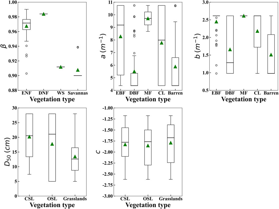
FIGURE 3. Root distribution parameters after optimization of 12 vegetation types (ENF = evergreen needleleaf forests, DNF = deciduous needleleaf forests, WS = woody savannas, savannas, EBF = evergreen broadleaf forests, DBF = deciduous broadleaf forests, MF = mixed forests, CL = Croplands, Barren = Barren, CSL = closed shrublands, OSL = open shrublands, Grasslands).

3.2 Vertical Distribution Characteristics of Root System of Twelve Vegetation Types

A statistical analysis of the data collected on the root distribution depth revealed that 94.5% of the plant root profile maximum depth is within 200 cm (Jackson et al., 1996; Schenk and Jackson, 2002a; Schenk and Jackson, 2002b). However, most of the collected articles did not specify the maximum root depth of the root profile (Schenk and Jackson, 2002a). Therefore, this study uses the maximum sampling depth of 200 cm as the maximum root depth to analyze the vertical distribution characteristics of the root system.

The processed data were compared to the root distribution curve obtained by optimizing the parameters of the root distribution ratio of 12 types of plantation in each layer (Figure 4). In general, the root distribution simulation curve (line) basically conforms to the changing trend of the measured data (point). The simulation curves are all single-peak curves. As the depth of the soil layer increases, the proportion of roots first increases and then decreases, and the peak value is often found at a depth of 10–20 cm. Although the proportion of roots of some vegetation in the measured data tends to decrease with increasing soil depth, a large number of research results show that the distribution of plant roots mainly increases with increasing soil depth, and the root distribution first increases and then decreases.

FIGURE 4

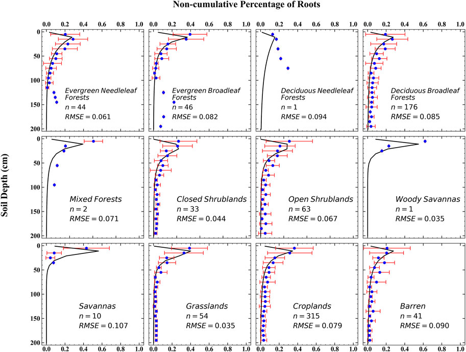
FIGURE 4. Observation data (the blue point is mean values, and the red line is SD) and simulation results (black line) of root distribution of 12 vegetation types.

The distribution ratio of shallow roots (0–30 cm) can reflect the depth of the root distribution to a certain extent; that is, the higher the ratio of shallow roots, the shallower the root distribution (Jackson et al., 1996). According to the simulation curve of the vertical distribution of roots of 12 vegetation types, the average distribution of the shallow roots is about 70.6%. In general, the root systems of the grassland (3 species) are relatively shallow, with an average shallow root system distribution rate of 89.6%. Trees (5 species) have a deep root distribution, with an average shallow root distribution ratio of 62.0%. The depth of shrubs and crops root distribution is between those of grasslands and trees. Among all vegetation types, savannas have the shallowest root system distribution, and the distribution ratio of the shallow root systems is 94.5%. The deciduous needleleaf forests have the deepest distribution of roots, and the distribution of shallow roots is 40.2%.

3.3 Overall Characteristics of ET_a, T_a, and E_a

The ET_a, T_a and E_a of China in 2015 were calculated based on the calculation of the SPAC model (Figure 5). The ET_a showed a gradually decreasing trend from southeast to northwest (Figure 5A), ranging from 18 to 1,172 mm/y, with an average value of 342.2 mm/y ± 244.2 mm/y, and a median value of 273.2 mm/y. The T_a range is between 0 and 700 mm/y, with an average value of 123.9 ± 98.1 mm/y, and the median value is 104.7 mm/y. The E_a in China exhibits prominent regional distribution characteristics, showing lower value in the Qinghai-Tibet Plateau and desert areas while highest in the semi-humid regions. The E_a range is 1–968 mm/y, with an average value of 218.3 ± 183.0 mm/y, and the median value is 161.2 mm/y, with a decreasing trend from southeast to northwest.

FIGURE 5

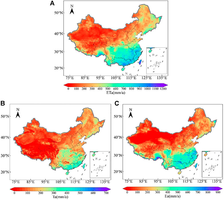
FIGURE 5. Spatial variations of (A) ET_a (mm/a) (B) T_a (mm/a), and (C) E_a (mm/a) of 2015 in China region.

3.4 ET_a of Different Vegetation Types

In 2015, the average ET_a order of nine different vegetation types in China’s land area was evergreen broadleaf forests (773 mm/y) > savannas (618 mm/y) > evergreen needleleaf forests (612 mm/y) > deciduous broadleaf forests (451 mm/y) > croplands (387 mm/y) > closed shrublands (287 mm/y)> grasslands (228 mm/y) > open shrublands (180 mm/y) > barren (151 mm/y) (Supplementary Table S2). The average ET_a of evergreen broadleaf forests is the highest, and the barren is the lowest. The ET_a of the three tropical and subtropical vegetation types, viz., evergreen broadleaf forests, savannas and evergreen needleleaf forests, are much higher than the ET_a of other vegetation types. The average ET_a of closed shrubs is much higher than that of open shrubs. It is also evident from Supplementary Table S2 that the average T_a (299 mm/y) and E_a (474 mm/y) of evergreen broadleaf forests are the highest. The average T_a (53 mm/y) of open shrublands and the average E_a of barren (85 mm/y) are the lowest. The average ET_a of open shrublands is higher than that of the barren, but the average T_a is lower than that of the barren. The average E_a of nine vegetation types is generally higher than the average T_a, a relatively large proportion. The average T_a accounted for about 24–51% of ET_a, and the average E_a accounted for 49–76% of ET_a. It should be noted that the ET_a of deciduous coniferous forests, mixed forests and woody savannas are not analyzed due to limited root systems data.

4 Discussion

4.1 Relationship Between Root Distribution Parameters and Environmental Factors

Among the three root distribution functions, the parameter β in the single factor function and $D_{50}$ in LDR function may reflect the depth of root distribution to a certain extent (Jackson et al., 1996; Schenk and Jackson, 2002a). Although the parameters a, b, and c do not directly reflect the depth of root distribution, they may also indirectly reflect the relationship to the root distribution by calculations. Therefore, this paper selects the four factors of mean annual temperature (MAT), mean annual precipitation (MAP), latitude, and altitude to analyze the correlation between plant root distribution parameters and explore the relationship between environmental factors and root distribution parameters.

The results showed that the parameter β has a significantly negative correlation with MAP and MAT, and a significantly positive correlation with latitude (Supplementary Table S3), which the correlation with the MAT is the largest (r = -0.845, p < 0.01). With increasing precipitation and temperature, the distribution of plant roots becomes shallower. As latitude increases, the temperature and precipitation decrease, and the distribution of plant roots become deeper. The parameter $D_{50}$ is negatively correlated with the average annual precipitation and has no significant correlation with the other three factors. It shows that the root distribution becomes shallower as precipitation increases. All root distribution parameters correlate significantly with MAP (p < 0.01), indicating that the influence of precipitation on root distribution is more significant than that of temperature and latitude. This trend may be because plants need to develop deeper roots to absorb water and nutrients in areas with low rainfall and relatively low soil moisture. On the contrary, in areas with high rainfall, the water content of the shallow soils is sufficient for plant growth and utilization, and the shallow root system can meet its growth needs (Fan et al., 2017). Some studies have shown that root distribution strongly correlates with soil moisture. Insufficient surface soil moisture capacity will cause roots to grow deeper to find water sources (Yu et al., 2007; Yu et al., 2015; Fan et al., 2017). The depth of water infiltration and the demand for evaporation are the main factors affecting the vertical distribution of root systems. Deep root systems are less likely to occur in humid areas (Dawson and Pate, 1996; Pregitzer et al., 2000; Powers and Peréz-Aviles, 2013; Fan et al., 2017). Previous studies have shown that in regions rich in water resources, the root distribution does not need to grow deeper but will still grow laterally, resulting in a larger proportion of shallow roots (Fan et al., 2017). However, the size of plant roots will increase with the increase in the aerial part of the plant, so that the tree roots are larger than shrub roots, and shrub roots are larger than grassroots (Schenk and Jackson, 2002b).

Parameters a and b have the same correlation, which is significantly positively correlated with MAP and MAT (p < 0.01) and significantly negatively correlated with latitude (p < 0.01). However, it is opposite to the correlation of parameters β. In the two-factor function, the larger a and b, the more shallow the root distribution. The parameter c in the LDR function reflects the plant type, which is significantly positively correlated with MAP (p < 0.01) and significantly negatively correlated with latitude (p < 0.05), indicating that the plant type has some correlation with MAP and latitude. For example, in the lower latitudes of southeast China, which is in a humid or semi-humid area, the vegetation mainly consists of tall trees (Su et al., 2015; Xiang et al., 2015). However, in the arid and semi-arid areas of high latitudes regions of northwest China, the vegetation is mainly shrubs, grasslands, and other low vegetation (Jia et al., 2012; Chen et al., 2017; Du et al., 2017).

Although the root distribution functions and parameters of different vegetation types were obtained in this study, there are also some differences in the root systems of the same plant under different growing environments. Multiple regression analyses on the root system distribution parameters and environmental factors were conducted, to quantify the relationship between each other (Supplementary Table S4). The results show that the adjustment R² of parameter β is the best ($R_{adj}^2$ = 0.631). Except for parameter c, the regression results for the remaining four parameters are Sig (P) < 0.001, indicating that the four fitted multiple linear regression equations are statistically significant when the significance level is 0.01. However, the equation does not consider some factors such as soil properties, vegetation characteristics and climate characteristics (Schenk and Jackson, 2002a; Laio et al., 2006). The results are uncertain but statistically significant. Therefore, it has a certain guiding significance.

4.2 Analysis of the Vertical Distribution Characteristics of Root System

The simulation results show that as the soil depth increases, the root ratio first increases, peaks around 10–20 cm, and gradually decreases (Figure 4). However, the measured root distribution has two trends. The first is that as the soil depth increases, the proportion of roots gradually decreases; the second is the same as the simulation results. It may be because, under the field measurement conditions, the amount of root coefficients is mainly based on range statistics (such as 0–10 cm, 0–20 cm). It is impossible to measure the proportion of the root system within 1cm, and it is impossible to accurately obtain the change in the surface layer (0–20 cm). Therefore, the measured data tends to decrease gradually. In addition, the distribution of plant roots will also be affected by the local climate, so that the plant roots will exhibit different distribution trends in different climate zones. Studies have shown that water infiltration depth and evaporation demand are the main factors affecting the vertical distribution of roots (Schenk and Jackson, 2002b), and root distribution have a strong correlation with soil moisture (Yu et al., 2015; Wang B. et al., 2016; Wang Y. et al., 2016). Soil moisture is a relevant independent variable in some root distribution models (Jarvis, 1989; Wu et al., 2020). Therefore, many field measurements of the root system show that the root system decreases as depth increases (Guo et al., 2016; Feng et al., 2017; Chen et al., 2018). Studies have also shown that the vertical distribution of roots first increases and then decreases (Hao et al., 2013; Jian et al., 2015; Li et al., 2015).

The vertical root distribution is usually assumed following a single-peak curve in the root distribution model. This trend can also be verified in the model where plants absorb water from the soil profile (Ojha and Rai, 1996; Wu et al., 1999; Li et al., 2010). In addition, Schenk and Jackson (2002a) pointed out that the average $D_{50}$ of global vegetation is mainly between 5 and 28 cm, indicating that the peak value of root systems of most vegetation in the world ranged is between 5–28 cm. It also proves that the simulated curve in this article may better reflect the actual trend of the root distribution than the measured data.

Of all vegetation types, crops are most affected by human activities (Schenk and Jackson, 2002a). However, this study did not consider the impact of human management practices on crops. The root distribution curve still has a good fit result (RMSE = 0.079) (Figure 4).

4.3 Estimation and Partition of ET_a

This study focuses on the ET_a of different vegetation types and does not consider and use water bodies and wetlands with high ET_a capacity. Therefore, the results may differ slightly from those of other studies. But the overall spatial distribution trend is consistent with other studies and has certain credibility. For example, it is evident from Figure 5 that the trend of ET_a results in 2015 is similar to previous studies, showing a decreasing trend from southeast to northwest (Li et al., 2017; Bai and Liu, 2018; Ma N. et al., 2019). The trend estimated from the GLEAM dataset (Bai and Liu, 2018) is most similar to our study.

While applying the SPAC model to regional simulation, this study also tried to partition the ET_a of China’s land area and obtained the spatial distribution of T_a and E_a. Among them, the spatial distribution trend of average T_a is similar to that of MAT, and the spatial distribution trend of average E_a is identical to that of MAP. The main reason is that temperature is the main factor controlling plant transpiration in this model, and precipitation is the main factor influencing soil evaporation. Gonzalez Miralles et al. (2011) obtained the spatial distribution of worldwide evaporation for the first time and found that the evaporation is the highest near the equator. The higher the latitude, the lower the evaporation. The general trend in China is that evaporation from the southeast is higher than from the northwest, which is consistent with this study.

This study shows that the average T_a in different vegetation regions in China’s terrestrial land accounts for about 36%, and the average E_a accounts for about 64%. Gu et al. (2018) estimated the worldwide ET of different biomes based on the optimized remote sensing method, and the T/ET range is between 0.29 and 0.72. Due to differences in the proportion of ET of different scales and ecosystems (Hu et al., 2009; Kool et al., 2014; Talsma et al., 2018), there are significant errors in the evaporation of soil estimated from each model (Talsma et al., 2018). Therefore, the results obtained in this research are consistent with Gu et al. (2018).

4.4 Impact Factors of ET_a for Different Vegetation Types

There are some differences in ET_a under different vegetation cover (Zhang et al., 2001; Peters et al., 2011; Yang et al., 2012; Zheng et al., 2016; Du et al., 2019). The maximum ET_a of the evergreen broad-leaved forest is 773 mm/y, and the minimum of barren is 151 mm/y. Perhaps this is because the evergreen broadleaf forests are mainly located in tropical and subtropical humid areas with sufficient water and energy, so the ET_a is the highest. The barren is primarily located in arid regions with high temperature, low precipitation, low soil water content, less vegetation, and weak transpiration and evaporation capacity. Therefore, ET_a of the barren is the lowest. Liu et al. (2010) estimated the ET_a under different land-use types in the Skeleton Creek urban area. The results showed that the ET from the forest was the highest, around 850mm, except for open water and wetlands. Li et al. (2017) studied the changes in ET under different vegetation, showing that the impact of deforestation on ET is much more significant than other types of land cover. It also reflects that the ET capacity of forests is much greater than that of other vegetation. Zhang et al. (2001) studied the relationship between vegetation change and average annual ET at the regional scale. They found that the ET in forested catchments is higher than in grassed catchments.

The ET_a under different vegetation types varies due to variation in climate types, geographic distribution and plant characteristics, and the main influencing factors will also change to some extent. Many studies have analyzed the influencing factors of ET_a in different regions and different vegetation types. The main influencing factors are precipitation, temperature, radiation, vegetation types, soil moisture, leaf area index, etc. (Liu et al., 2019; Lu et al., 2011; Ma Z. et al., 2019; Peel et al., 2010; Sun et al., 2020; Zhang et al., 2001). Studies have shown that precipitation is the main factor affecting the actual spatial distribution of ET in the arid and semi-arid regions of northwest and northeast China. In the humid and semi-humid areas of southeast China, shortwave radiation, precipitation, temperature, and soil moisture are the main controlling factors (Sun et al., 2020). Therefore, according to the ET_a estimation results of different vegetation types, this paper examines the main factors influencing the ET_a under different vegetation types through correlation analysis. The results are shown in Figure 6. It is evident from the results that the four influencing factors were significantly correlated with the actual annual ET of nine vegetation types. The precipitation and the ET_a of all vegetation were significantly positively correlated (p < 0.01) and impacted all vegetation types considerably. The results show that among the four factors, precipitation has the most significant impact on the ET_a, and it is the main factor affecting the ET of the nine vegetation types (Zhang et al., 2001). Except for evergreen needleleaf forests, evergreen broadleaf forests and open shrubs, latitude has a significant negative correlation with other vegetation types, which may be related to the correlation between latitude and types of climate. Except for precipitation, the temperature significantly negatively correlates with most vegetation types (p < 0.01). However, the correlation coefficients between temperature and other vegetation are generally low (|r|<0.2) except for closed shrublands (|r| = 0.663).

FIGURE 6

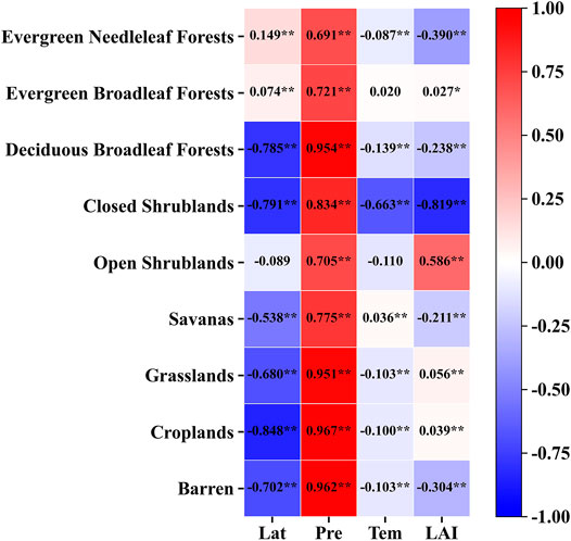
FIGURE 6. Correlation analysis between ET_a of different vegetation types and influencing factors. ∗p < 0.05, ∗∗p < 0.01. Lat (latitude); Pre (precipitation); Tem (temperature); LAI.

In addition to these influencing factors, plant physiological characteristics and soil texture also affect the ET capacity of plants (Schenk and Jackson, 2002a; Xue et al., 2020). Some studies have shown that the available water content of plants and the morphology of the plant growth somehow affect ET (Zhang et al., 2001; Kotani and Sugita, 2005; Balogun et al., 2009). The soil texture (such as sand, silt or clay) where vegetation grows affects water infiltration, which in turn affects the plant root depth (Fan et al., 2017), and also has some impact on ET_a (Schenk and Jackson, 2002a).

5 Conclusion

The data collected in this study have obtained parameters that can accurately simulate the vertical distribution of different vegetation roots in China, with a high precision of fit (RMSE = 0.035–0.107). It has a wide range of applicability in mainland China and has some benchmark significance for estimating the ET_a.

A SPAC model was built based on the optimized parameters, which improved the root water absorption module, and calculated the ET_a of different vegetation types. The results showed that evergreen broadleaf forests (773 mm/y) > savannas (618 mm/y) > evergreen needleleaf forests (612 mm/y) > deciduous broadleaf forests (451 mm/y) > croplands (387 mm/y) > closed shrublands (287 mm/y) > grasslands (228 mm/y) > open shrublands (180 mm/y) > barren (151 mm/y).

The spatial distribution of T_a and E_a in mainland China was calculated through the SPAC model. The spatial distribution trend of T_a and E_a are the same as the ET_a, and both show a decreasing trend from southeast to northwest. Among them, the ratio of average T_a to average E_a is 9/16.

Data Availability Statement

The raw data supporting the conclusion of this article will be made available by the authors, without undue reservation.

Author Contributions

ZD collected the data, designed the analysis and drafted the manuscript. HH and YL provided a conception of the work and critical revision of the manuscript. ZW and LC provided critical revision of the manuscript. HX, HY, and HL collected the data. MK provided a revision of the manuscript.

Funding

The project was supported by the National Key Research and Development Program of China (2018YFC1508102 and 2018YFC1508103), the National Natural Science Foundation of China (51879136 and 51809173), the Second Tibetan Plateau Scientific Expedition and Research Program (2019QZKK0207), and Water Conservancy Science and Technology Innovation Project in Guangdong Province (202012).

Conflict of Interest

The authors declare that the research was conducted in the absence of any commercial or financial relationships that could be construed as a potential conflict of interest.

Publisher’s Note

All claims expressed in this article are solely those of the authors and do not necessarily represent those of their affiliated organizations, or those of the publisher, the editors and the reviewers. Any product that may be evaluated in this article, or claim that may be made by its manufacturer, is not guaranteed or endorsed by the publisher.

Supplementary Material

The Supplementary Material for this article can be found online at: https://www.frontiersin.org/articles/10.3389/feart.2022.893388/full#supplementary-material

References

Allen, R. G., Pereira, L. S., Raes, D., and Smith, M. (1998). Crop Evapotranspiration-Guidelines for Computing Crop Water Requirements-FAO Irrigation and Drainage Paper 56. Rome: Fao.

Google Scholar

Bai, P., and Liu, X. (2018). Intercomparison and Evaluation of Three Global High-Resolution Evapotranspiration Products across China. J. Hydrology 566, 743–755. doi:10.1016/j.jhydrol.2018.09.065

CrossRef Full Text | Google Scholar

Balogun, A. A., Adegoke, J. O., Vezhapparambu, S., Mauder, M., McFadden, J. P., and Gallo, K. (2009). Surface Energy Balance Measurements above an Exurban Residential Neighbourhood of Kansas City, Missouri. Boundary-Layer Meteorol. 133, 299–321. doi:10.1007/s10546-009-9421-3

CrossRef Full Text | Google Scholar

Belmans, C., Wesseling, J. G., and Feddes, R. A. (1983). Simulation Model of the Water Balance of a Cropped Soil: SWATRE. J. hydrology 63, 271–286. doi:10.1016/0022-1694(83)90045-8

CrossRef Full Text | Google Scholar

Canadell, J., Jackson, R. B., Ehleringer, J. B., Mooney, H. A., Sala, O. E., and Schulze, E.-D. (1996). Maximum Rooting Depth of Vegetation Types at the Global Scale. Oecologia 108, 583–595. doi:10.1007/bf00329030

PubMed Abstract | CrossRef Full Text | Google Scholar

Chen, J., Wang, P., Ma, Z., Lyu, X., Liu, T.-t., and Siddique, K. H. M. (2018). Optimum Water and Nitrogen Supply Regulates Root Distribution and Produces High Grain Yields in Spring Wheat ( Triticum aestivum L.) under Permanent Raised Bed Tillage in Arid Northwest China. Soil Tillage Res. 181, 117–126. doi:10.1016/j.still.2018.04.012

CrossRef Full Text | Google Scholar

Chen, Y.-L., Zhang, Z.-S., Huang, L., Zhao, Y., Hu, Y.-G., Zhang, P., et al. (2017). Co-variation of Fine-Root Distribution with Vegetation and Soil Properties along a Revegetation Chronosequence in a Desert Area in Northwestern China. CATENA 151, 16–25. doi:10.1016/j.catena.2016.12.004

CrossRef Full Text | Google Scholar

Dawson, T. E., and Pate, J. S. (1996). Seasonal Water Uptake and Movement in Root Systems of Australian Phraeatophytic Plants of Dimorphic Root Morphology: a Stable Isotope Investigation. Oecologia 107, 13–20. doi:10.1007/bf00582230

PubMed Abstract | CrossRef Full Text | Google Scholar

Du, T., Wang, L., Yuan, G., Sun, X., and Wang, S. (2019). Effects of Distinguishing Vegetation Types on the Estimates of Remotely Sensed Evapotranspiration in Arid Regions. Remote Sens. 11, 2856. doi:10.3390/rs11232856

CrossRef Full Text | Google Scholar

Du, Z., Cai, Y., Yan, Y., and Wang, X. (2017). Embedded Rock Fragments Affect Alpine Steppe Plant Growth, Soil Carbon and Nitrogen in the Northern Tibetan Plateau. Plant Soil 420, 79–92. doi:10.1007/s11104-017-3376-9

CrossRef Full Text | Google Scholar

Fan, J., McConkey, B., Wang, H., and Janzen, H. (2016). Root Distribution by Depth for Temperate Agricultural Crops. Field Crops Res. 189, 68–74. doi:10.1016/j.fcr.2016.02.013

CrossRef Full Text | Google Scholar

Fan, Y., Miguez-Macho, G., Jobbágy, E. G., Jackson, R. B., and Otero-Casal, C. (2017). Hydrologic Regulation of Plant Rooting Depth. Proc. Natl. Acad. Sci. U.S.A. 114, 10572–10577. doi:10.1073/pnas.1712381114

PubMed Abstract | CrossRef Full Text | Google Scholar

Feddes, R. A., and Zaradny, H. (1978). Model for Simulating Soil-Water Content Considering Evapotranspiration - Comments. J. Hydrology 37, 393–397. doi:10.1016/0022-1694(78)90030-6

CrossRef Full Text | Google Scholar

Feng, S., Gu, S., Zhang, H., and Wang, D. (2017). Root Vertical Distribution Is Important to Improve Water Use Efficiency and Grain Yield of Wheat. Field Crops Res. 214, 131–141. doi:10.1016/j.fcr.2017.08.007

CrossRef Full Text | Google Scholar

Flerchinger, G. N. (2000). The Simultaneous Heat and Water (SHAW) Model: Technical Documentation. Boise, Idaho: Northwest Watershed Research Center USDA Agricultural Research Service.

Google Scholar

Friedl, M. A., Sulla-Menashe, D., Tan, B., Schneider, A., Ramankutty, N., Sibley, A., et al. (2010). MODIS Collection 5 Global Land Cover: Algorithm Refinements and Characterization of New Datasets. Remote Sens. Environ. 114, 168–182. doi:10.1016/j.rse.2009.08.016

CrossRef Full Text | Google Scholar

Gale, M. R., and Grigal, D. F. (1987). Vertical Root Distributions of Northern Tree Species in Relation to Successional Status. Can. J. For. Res. 17, 829–834. doi:10.1139/x87-131

CrossRef Full Text | Google Scholar

Gu, C., Ma, J., Zhu, G., Yang, H., Zhang, K., Wang, Y., et al. (2018). Partitioning Evapotranspiration Using an Optimized Satellite-Based ET Model across Biomes. Agric. For. meteorology 259, 355–363. doi:10.1016/j.agrformet.2018.05.023

CrossRef Full Text | Google Scholar

Guo, F., Ma, J.-j., Zheng, L.-j., Sun, X.-h., Guo, X.-h., and Zhang, X.-l. (2016). Estimating Distribution of Water Uptake with Depth of Winter Wheat by Hydrogen and Oxygen Stable Isotopes under Different Irrigation Depths. J. Integr. Agric. 15, 891–906. doi:10.1016/S2095-3119(15)61258-8

CrossRef Full Text | Google Scholar

Hao, X.-M., Chen, Y.-N., Guo, B., and Ma, J.-X. (2013). Hydraulic Redistribution of Soil Water inPopulus euphraticaOliv. In a Central Asian Desert Riparian Forest. Ecohydrol. 6, 974–983. doi:10.1002/eco.1338

CrossRef Full Text | Google Scholar

Hu, Z., Yu, G., Zhou, Y., Sun, X., Li, Y., Shi, P., et al. (2009). Partitioning of Evapotranspiration and its Controls in Four Grassland Ecosystems: Application of a Two-Source Model. Agric. For. Meteorology 149, 1410–1420. doi:10.1016/j.agrformet.2009.03.014

CrossRef Full Text | Google Scholar

Jackson, R. B., Canadell, J., Ehleringer, J. R., Mooney, H. A., Sala, O. E., and Schulze, E. D. (1996). A Global Analysis of Root Distributions for Terrestrial Biomes. Oecologia 108, 389–411. doi:10.1007/bf00333714

PubMed Abstract | CrossRef Full Text | Google Scholar

Jackson, R. B., Mooney, H. A., and Schulze, E.-D. (1997). A Global Budget for Fine Root Biomass, Surface Area, and Nutrient Contents. Proc. Natl. Acad. Sci. U.S.A. 94, 7362–7366. doi:10.1073/pnas.94.14.7362

PubMed Abstract | CrossRef Full Text | Google Scholar

Jarvis, N. J. (1989). A Simple Empirical Model of Root Water Uptake. J. Hydrology 107, 57–72. doi:10.1016/0022-1694(89)90050-4

CrossRef Full Text | Google Scholar

Jia, Z., Zhu, Y., and Liu, L. (2012). Different Water Use Strategies of Juvenile and Adult Caragana Intermedia Plantations in the Gonghe Basin, Tibet Plateau. Plos One 7, e45902. doi:10.1371/journal.pone.0045902

PubMed Abstract | CrossRef Full Text | Google Scholar

Jian, S. Q., Zhao, C. Y., Fang, S. M., and Yu, K. (2015). The Distribution of Fine Root Length Density for Six Artificial Afforestation Tree Species in Loess Plateau of Northwest China. For. Syst. 24, 3. doi:10.5424/fs/2015241-05521

CrossRef Full Text | Google Scholar

Kennedy, J., and Neville, A. (1986). Statistical Methods for Engineers and Scientist. London: pub Harper and Row.

Google Scholar

Kool, D., Agam, N., Lazarovitch, N., Heitman, J. L., Sauer, T. J., and Ben-Gal, A. (2014). A Review of Approaches for Evapotranspiration Partitioning. Agric. For. meteorology 184, 56–70. doi:10.1016/j.agrformet.2013.09.003

CrossRef Full Text | Google Scholar

Kotani, A., and Sugita, M. (2005). Seasonal Variation of Surface Fluxes and Scalar Roughness of Suburban Land Covers. Agric. For. meteorology 135, 1–21. doi:10.1016/j.agrformet.2005.09.012

CrossRef Full Text | Google Scholar

Kumar, R., Shankar, V., and Jat, M. K. (2015). Evaluation of Root Water Uptake Models - a Review. ISH J. Hydraulic Eng. 21, 115–124. doi:10.1080/09715010.2014.981955

CrossRef Full Text | Google Scholar

Laio, F., D'Odorico, P., and Ridolfi, L. (2006). An Analytical Model to Relate the Vertical Root Distribution to Climate and Soil Properties. Geophys. Res. Lett. 33. doi:10.1029/2006gl027331

CrossRef Full Text | Google Scholar

Li, B., Wang, J. F., Wang, J., Ren, X., Bao, L., Zhang, L., et al. (2015). Root Growth, Yield and Fruit Quality of 'Red Fuji' Apple Trees in Relation to Planting Depth of Dwarfing Interstock on the Loess Plateau. Eur. J. Hort. Sci. 80, 109–116. doi:10.17660/ejhs.2015/80.3.3

CrossRef Full Text | Google Scholar

Li, G., Zhang, F., Jing, Y., Liu, Y., and Sun, G. (2017). Response of Evapotranspiration to Changes in Land Use and Land Cover and Climate in China during 2001-2013. Sci. Total Environ. 596-597, 256–265. doi:10.1016/j.scitotenv.2017.04.080

PubMed Abstract | CrossRef Full Text | Google Scholar

Li, J., Zhao, C. Y., Song, Y. J., Sheng, Y., and Zhu, H. (2010). Spatial Patterns of Desert Annuals in Relation to Shrub Effects on Soil Moisture. J. Veg. Sci. 21, 221–232. doi:10.1111/j.1654-1103.2009.01135.x

CrossRef Full Text | Google Scholar

Liu, W., Hong, Y., Khan, S. I., Huang, M., Vieux, B., Caliskan, S., et al. (2010). Actual Evapotranspiration Estimation for Different Land Use and Land Cover in Urban Regions Using Landsat 5 Data. J. Appl. Remote Sens. 4, 041873. doi:10.1117/1.3525566

CrossRef Full Text | Google Scholar

Liu, Y. J., Chen, J., and Pan, T. (2019). Analysis of Changes in Reference Evapotranspiration, Pan Evaporation, and Actual Evapotranspiration and Their Influencing Factors in the North China Plain during 1998-2005. Earth Space Sci. 6, 1366–1377. doi:10.1029/2019ea000626

CrossRef Full Text | Google Scholar

Lu, N., Chen, S., Wilske, B., Sun, G., and Chen, J. (2011). Evapotranspiration and Soil Water Relationships in a Range of Disturbed and Undisturbed Ecosystems in the Semi-arid Inner Mongolia, China. J. Plant Ecol. 4, 49–60. doi:10.1093/jpe/rtq035

CrossRef Full Text | Google Scholar

Ma, N., Szilagyi, J., Zhang, Y., and Liu, W. (2019a). Complementary‐Relationship‐Based Modeling of Terrestrial Evapotranspiration across China during 1982-2012: Validations and Spatiotemporal Analyses. J. Geophys. Res. Atmos. 124, 4326–4351. doi:10.1029/2018jd029850

CrossRef Full Text | Google Scholar

Ma, Z., Yan, N., Wu, B., Stein, A., Zhu, W., and Zeng, H. (2019b). Variation in Actual Evapotranspiration Following Changes in Climate and Vegetation Cover during an Ecological Restoration Period (2000-2015) in the Loess Plateau, China. Sci. total Environ. 689, 534–545. doi:10.1016/j.scitotenv.2019.06.155

PubMed Abstract | CrossRef Full Text | Google Scholar

Miralles, D. G., Holmes, T. R. H., De Jeu, R. A. M., Gash, J. H., Meesters, A. G. C. A., and Dolman, A. J. (2011). Global Land-Surface Evaporation Estimated from Satellite-Based Observations. Hydrol. Earth Syst. Sci. 15, 453–469. doi:10.5194/hess-15-453-2011

CrossRef Full Text | Google Scholar

Nepstad, D. C., de Carvalho, C. R., Davidson, E. A., Jipp, P. H., Lefebvre, P. A., Negreiros, G. H., et al. (1994). The Role of Deep Roots in the Hydrological and Carbon Cycles of Amazonian Forests and Pastures. Nature 372, 666–669. doi:10.1038/372666a0

CrossRef Full Text | Google Scholar

Ojha, C. S. P., and Rai, A. K. (1996). Nonlinear Root-Water Uptake Model. J. irrigation drainage Eng. 122, 198–202. doi:10.1061/(asce)0733-9437(1996)122:4(198)

CrossRef Full Text | Google Scholar

Peel, M. C., McMahon, T. A., and Finlayson, B. L. (2010). Vegetation Impact on Mean Annual Evapotranspiration at a Global Catchment Scale. Water Resour. Res. 46, W09508. doi:10.1029/2009wr008233

CrossRef Full Text | Google Scholar

Peters, E. B., Hiller, R. V., and McFadden, J. P. (2011). Seasonal Contributions of Vegetation Types to Suburban Evapotranspiration. J. Geophys. Res. Biogeosciences 116, 1463. doi:10.1029/2010jg001463

CrossRef Full Text | Google Scholar

Philip, J. R. (1966). Plant Water Relations: Some Physical Aspects. Annu. Rev. Plant. Physiol. 17, 245–268. doi:10.1146/annurev.pp.17.060166.001333

CrossRef Full Text | Google Scholar

Powers, J. S., and Peréz-Aviles, D. (2013). Edaphic Factors Are a More Important Control on Surface Fine Roots Than Stand Age in Secondary Tropical Dry Forests. Biotropica 45, 1–9. doi:10.1111/j.1744-7429.2012.00881.x

CrossRef Full Text | Google Scholar

Pregitzer, K. S., King, J. S., Burton, A. J., and Brown, S. E. (2000). Responses of Tree Fine Roots to Temperature. New Phytol. 147, 105–115. doi:10.1046/j.1469-8137.2000.00689.x

CrossRef Full Text | Google Scholar

Richards, L. A. (1931). Capillary Conduction of Liquids through Porous Mediums. Physics 1, 318–333. doi:10.1063/1.1745010

CrossRef Full Text | Google Scholar

Schenk, H. J., and Jackson, R. B. (2002b). Rooting Depths, Lateral Root Spreads and Below‐ground/above‐ground Allometries of Plants in Water‐limited Ecosystems. J. Ecol. 90, 480–494. doi:10.1046/j.1365-2745.2002.00682.x

CrossRef Full Text | Google Scholar

Schenk, H. J., and Jackson, R. B. (2002a). The Global Biogeography of Roots. Ecol. Monogr. 72, 311–328. doi:10.1890/0012-9615(2002)072[0311:tgbor]2.0.co;2

CrossRef Full Text | Google Scholar

Shangguan, W., Dai, Y., Liu, B., Zhu, A., Duan, Q., Wu, L., et al. (2013). A China Data Set of Soil Properties for Land Surface Modeling. J. Adv. Model. Earth Syst. 5, 212–224. doi:10.1002/jame.20026

CrossRef Full Text | Google Scholar

Su, W., Liu, B., Liu, X., Li, X., Ren, T., Cong, R., et al. (2015). Effect of Depth of Fertilizer Banded-Placement on Growth, Nutrient Uptake and Yield of Oilseed Rape (Brassica Napus L.). Eur. J. Agron. 62, 38–45. doi:10.1016/j.eja.2014.09.002

CrossRef Full Text | Google Scholar

Sun, S., Song, Z., Chen, X., Wang, T., Zhang, Y., Zhang, D., et al. (2020). Multimodel‐based Analyses of Evapotranspiration and its Controls in China over the Last Three Decades. Ecohydrology 13, 2195. doi:10.1002/eco.2195

CrossRef Full Text | Google Scholar

Sweeney, J. (1997). “The International Geosphere-Biosphere Programme in Global Change and the Irish Environment. Irish Committee for IGBP (Ireland: IGBP).

Google Scholar

Talsma, C. J., Good, S. P., Jimenez, C., Martens, B., Fisher, J. B., Miralles, D. G., et al. (2018). Partitioning of Evapotranspiration in Remote Sensing-Based Models. Agric. For. Meteorology 260-261, 131–143. doi:10.1016/j.agrformet.2018.05.010

CrossRef Full Text | Google Scholar

Van Genuchten, M. T. (1980). A Closed-form Equation for Predicting the Hydraulic Conductivity of Unsaturated Soils. Soil Sci. Soc. Am. J. 44, 892–898. doi:10.2136/sssaj1980.03615995004400050002x

CrossRef Full Text | Google Scholar

Wang, B., Zheng, L. J., Ma, J. J., Sun, X. H., Guo, X. H., and Guo, F. (2016a). Effective Root Depth and Water Uptake Ability of Winter Wheat by Using Water Stable Isotopes in the Loess Plateau of China. Int. J. Agric. Biol. Eng. 9, 27–35. doi:10.3965/j.ijabe.20160906.2450

CrossRef Full Text | Google Scholar

Wang, Y., Zhu, Q. K., Zhao, W. J., Ma, H., Wang, R., and Ai, N. (2016b). The Dynamic Trend of Soil Water Content in Artificial Forests on the Loess Plateau, China. Forests 7, 236. doi:10.3390/f7100236

CrossRef Full Text | Google Scholar

Wu, J., Zhang, R., and Gui, S. (1999). Modeling Soil Water Movement with Water Uptake by Roots. Plant Soil 215, 7–17. doi:10.1023/a:1004702807951

CrossRef Full Text | Google Scholar

Wu, X., Zuo, Q., Shi, J., Wang, L., Xue, X., and Ben-Gal, A. (2020). Introducing Water Stress Hysteresis to the Feddes Empirical Macroscopic Root Water Uptake Model. Agric. Water Manag. 240, 106293. doi:10.1016/j.agwat.2020.106293

CrossRef Full Text | Google Scholar

Xiang, W., Fan, G., Lei, P., Zeng, Y., Tong, J., Fang, X., et al. (2015). Fine Root Interactions in Subtropical Mixed Forests in China Depend on Tree Species Composition. Plant Soil 395, 335–349. doi:10.1007/s11104-015-2573-7

CrossRef Full Text | Google Scholar

Xue, B., Wang, G., Xiao, J., Tan, Q., Shrestha, S., Sun, W., et al. (2020). Global Evapotranspiration Hiatus Explained by Vegetation Structural and Physiological Controls. Ecol. Eng. 158, 106046. doi:10.1016/j.ecoleng.2020.106046

CrossRef Full Text | Google Scholar

Yang, K., and He, J. (2019). China Meteorological Forcing Dataset (1979-2018). National Tibetan Plateau Data Center. doi:10.11888/AtmosphericPhysics.tpe.249369.file

CrossRef Full Text | Google Scholar

Yang, X., Ren, L., Singh, V. P., Liu, X., Yuan, F., Jiang, S., et al. (2012). Impacts of Land Use and Land Cover Changes on Evapotranspiration and Runoff at Shalamulun River Watershed, China. Hydrology Res. 43, 23–37. doi:10.2166/nh.2011.120

CrossRef Full Text | Google Scholar

Yang, Y., Fang, J., Ji, C., and Han, W. (2009). Above- and Belowground Biomass Allocation in Tibetan Grasslands. J. Veg. Sci. 20, 177–184. doi:10.1111/j.1654-1103.2009.05566.x

CrossRef Full Text | Google Scholar

Yu, G.-R., Zhuang, J., Nakayama, K., and Jin, Y. (2007). Root Water Uptake and Profile Soil Water as Affected by Vertical Root Distribution. Plant Ecol. 189, 15–30. doi:10.1007/s11258-006-9163-y

CrossRef Full Text | Google Scholar

Yu, W.-q., Wang, Y.-j., Hu, H.-b., Wang, Y.-q., Zhang, H.-l., Wang, B., et al. (2015). Regulations and Patterns of Soil Moisture Dynamics and Their Controlling Factors in Hilly Regions of Lower Reaches of Yangtze River Basin, China. J. Cent. South Univ. 22, 4764–4777. doi:10.1007/s11771-015-3028-2

CrossRef Full Text | Google Scholar

Zeng, X., Dai, Y.-J., Dickinson, R. E., and Shaikh, M. (1998). The Role of Root Distribution for Climate Simulation over Land. Geophys. Res. Lett. 25, 4533–4536. doi:10.1029/1998gl900216

CrossRef Full Text | Google Scholar

Zeng, X. (2001). Global Vegetation Root Distribution for Land Modeling. J. Hydrometeor 2, 525–530. doi:10.1175/1525-7541(2001)002<0525:gvrdfl>2.0.co;2

CrossRef Full Text | Google Scholar

Zhang, L., Dawes, W. R., and Walker, G. R. (2001). Response of Mean Annual Evapotranspiration to Vegetation Changes at Catchment Scale. Water Resour. Res. 37, 701–708. doi:10.1029/2000wr900325

CrossRef Full Text | Google Scholar

Zheng, H., Yu, G., Wang, Q., Zhu, X., He, H., Wang, Y., et al. (2016). Spatial Variation in Annual Actual Evapotranspiration of Terrestrial Ecosystems in China: Results from Eddy Covariance Measurements. J. Geogr. Sci. 26, 1391–1411. doi:10.1007/s11442-016-1334-8

CrossRef Full Text | Google Scholar