Global navigation satellite system technology has been widely used for high-precision, real-time monitoring of landslides. To improve forecasts and early warnings, the true deformation features must be extracted from the global navigation satellite system monitoring series. However, as the deformation rate changes at different creep stages, the relationship between noise and true deformation may also change, making it difficult to accurately describe the deformation. In this study, an adaptive sliding window algorithm is proposed to account for this relationship change. First, the window was defined with an equal window width and step length, which improved the efficiency of feature extraction. Second, the median and normalized interquartile ranges were used to estimate the window samples and obtain a continuous and reliable series. Finally, the window sample breakdown point was defined to adjust the window parameter. These steps were repeated for the adjusted window to achieve adaptive processing of the monitoring series. The results based on both simulated and real landslide monitoring series demonstrated that the proposed method can provide adaptive, robust, and reliable deformation information for landslide warnings. The adaptive sliding window method also successfully assisted in the early warning of a loess landslide in Heifangtai, Gansu province, northwest of the Chinese Loess Plateau, indicating its practical application potential.

1 Introduction

Many countries worldwide suffer from recurring geological disasters, particularly landslides, and the loss of life and property caused by landslides has increased each year (Froude and Petley, 2018). Because of the complexity of landslides, predicting the failure time of a landslide remains challenging. Previous studies showed that most landslides conform to a three-stage creep curve from the initial to final failures (Tavenas and Leroueil, 1981; Dok et al., 2011). According to the creep curve interpretation, the first stage is primary creep, in which the strain rate decreases logarithmically, followed by steady-state creep with a constant strain rate and accelerating creep with an increasing creep rate that leads to rupture (Figure 1). For a three-stage creep curve, time-to-failure predictions can be made using existing methods (Xu et al., 2011; Intrieri et al., 2019). The global navigation satellite system (GNSS), which captures global, continuous, and high-precision geospatial data, has been widely used for monitoring landslides and obtaining creep curves (Benoit et al., 2014; Du et al., 2020). However, GNSS positioning technology is often affected by the external environment, multipath effect, atmospheric delay, receiver noise, and other hardware influences, causing the monitoring series to create noise (Amiri-Simkooei, 2008; Li et al., 2016; Han et al., 2018).

FIGURE 1

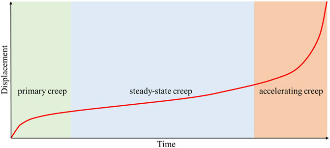
FIGURE 1. Conventional three-state interpretation of landslide creep behavior, Shaded areas of different colors represent different stages.

Various methods have been applied to preprocess landslide monitoring series to reduce the effect of noise and improve prediction accuracy. Kalman filtering is a method used to describe the dynamic deformation process of a monitoring body by calculating the optimal value of the state vector. However, the GNSS monitoring series includes colored noise, which cannot satisfy the white-noise assumption of the Kalman filter (Ince and Sahin, 2000; Li and Kuhlmann, 2013; Zhao et al., 2016). The wavelet analysis method decomposes the different frequency components of the signal and extracts useful deformation information from the series. However, wavelet analysis is used for data series of equal intervals and cannot be directly used for data of non-equal intervals. Additionally, the preprocessing methods depend on the experience of those implementing the method (Yang et al., 2012). The sliding window method applies a finite time window to select the dataset for preprocessing. The window is then incrementally moved forward in time, resulting in estimates for each window (Song and Lee, 2015; Banerjee and Bansal, 2017). Based on sliding-window methods, various creep curve features, such as deformation speed, tangential angle, and acceleration, are widely used for deformation feature extraction in GNSS landslide monitoring series because of the need for a certain time interval.

The conventional sliding-window method with fixed coefficients is typically applied to extract the signal if the mean and covariance of the dataset do not change as the window moves. Inevitably, as the landslide evolves, the true deformation increases and gradually occupies the main component of the monitoring results, and the mean and covariance of the dataset constantly change. Thus, window estimation can lead to errors and reduce the real-time performance of monitoring. Therefore, as the true deformation changes, preprocessing strategies should be considered. Ren et al. evaluated the moving average method only for a slow deformation monitoring sequence (Ren and Xu, 2018). Zhu et al. proposed a self-adaptive data-acquisition method to dynamically adjust the output rate of the sensor to reduce the power consumption of the sensor node (Zhu et al., 2017). However, the crucial threshold delta of the method must be set manually and the processing window kept fixed. In this study, we present a new technology for adaptive adjustment of sliding-window coefficients based on the window sample breakdown point. This method may capture the entire displacement feature of a landslide failure in a timely manner and assist in further early warning.

We first describe the sliding-window technology; the concept of the sample breakdown point is then introduced to derive the technical process of the method. Next, the simulation experiment results are presented to demonstrate the performance of the sliding-window approach for different outliers and deformation signals. The efficiency of this approach was validated using a GNSS monitoring series, collected during displacement monitoring of the Heifangtai landslide.

2 Materials and Methods

2.1 Fundamental Sliding-Window Parameters

The sliding window uses a time window to select the data for processing and steps forward in regular increments to obtain a series of estimates (Foster et al., 2005). Three parameters are required to define a window: 1) position of the window, 2) width of the window, and 3) the step by which the window moves forward. For a GNSS monitoring series with duration of T, the window position is defined as t, which is the central time of the window. In this case, the processing result is closest to the real deformation in that window.

The “width” of the window can be specified by the time width (W), which determines the efficiency of sample estimation in the window. A wider selected window contains more observations and gives a more reliable estimation than a narrower window. In contrast, because the position is the center of the window, increasing the width causes a lag $\left({\mathit{\tau }}_{\mathit{t}}\right)$ in the window position (window position later than real data time):

$\begin{array}{c}{\mathit{\tau }}_{\mathit{t}}=\frac{\mathit{W}}{\mathbf{2}}\end{array},(1)$

The “step” by which the window moves forward can be specified by the time step (S), which determines when the window is obtained. It is possible to use either of the options: step-by-step or equal to the width. In the former option, the window is moved forward in steps, generating a full solution for each step. Since each epoch participates in the estimation of multiple windows, the option may lead to correlations between the different estimates (Figure 2A). In the equal option, the window moves forward in multiple steps and the estimated values are independent of each other (Figure 2B). The final number of estimates (N) was determined using Eq. 2:

$\begin{array}{c}\mathit{N}=\mathit{f}\mathit{l}\mathit{o}\mathit{o}\mathit{r}\left(\frac{\mathit{T}-\mathit{W}}{\mathit{S}}\right)+\mathbf{1}\end{array},(2)$

where “floor” indicates that the resultant is rounded to the nearest integer. According to the equation, an increase in the step length reduces the final number of estimates, which can be used to extract more useful features from the original series. In this study, we focused on the second option, which avoids correlation and provides a regularly spaced feature series for pre-warning analysis of landslides.

FIGURE 2

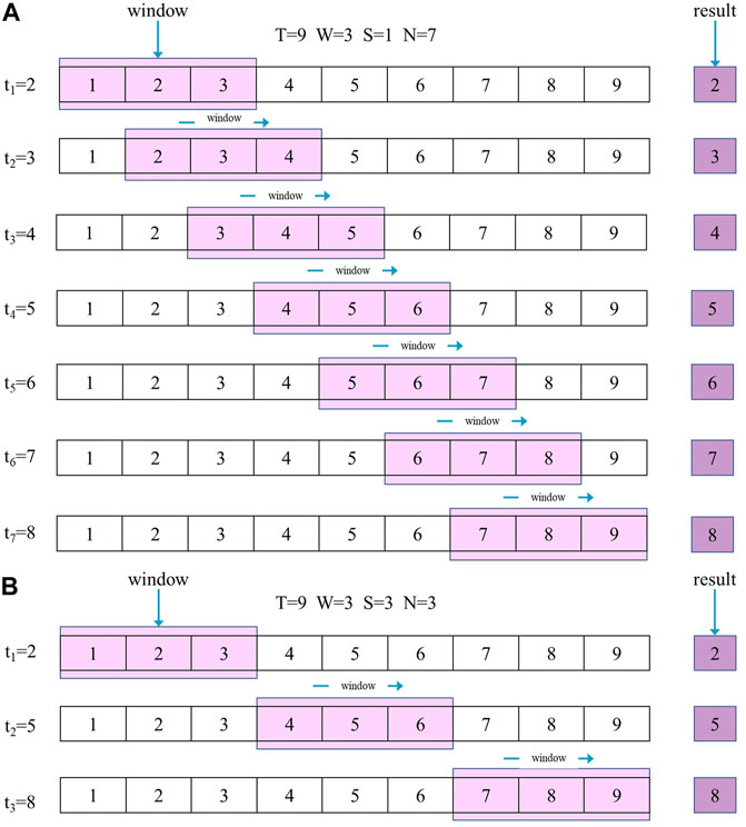
FIGURE 2. Schematic diagram of a sliding-window process. The position of the window is the center time. (A) Step option 1: step by step; (B) Step option 2: equal with the width.

2.2 Window Sample Estimation

The window sample was estimated after defining the window. The sliding window method typically uses the sample mean and standard deviation as estimators. The method can obtain an optimal estimation result only when the window sample shows a normal distribution. For real monitoring data, a window sample affected by outliers and deformation may not meet this condition. Using the median and normalized interquartile range (NIQR) is another robust method for estimating the average and standard deviation of the window sample. This method is suitable for estimating symmetric and skewed distributions (Buch, 2014). If $\mathit{X}$ is a sample with values ${\mathit{x}}_{\mathbf{1}}, {\mathit{x}}_{\mathbf{2}},\dots ,{\mathit{x}}_{\mathit{n}}$, then the median is calculated as shown in Eq. 3.

$\begin{array}{c}\mathit{m}\mathit{e}\mathit{d}\left(\mathit{X}\right)=\{\begin{array}{c}{\mathit{x}}_{\left(\mathit{i}+\mathbf{1}\right)}\left(\mathit{n}=\mathbf{2}\mathit{i}+\mathbf{1}\right)\\ \left({\mathit{x}}_{\left(\mathit{i}\right)}+{\mathit{x}}_{\left(\mathit{i}+\mathbf{1}\right)}\right)/\mathbf{2}\left(\mathit{n}=\mathbf{2}\mathit{i}\right)\end{array}\end{array}(3)$

where $\mathit{i}$ is the sorted value of the dataset. NIQR can be defined as shown in Eq. 4 (Fried and Gather, 2007).

$\begin{array}{c}\mathit{N}\mathit{I}\mathit{Q}\mathit{R}=\mathbf{0.7413}\times \left({\mathit{Q}}_{\mathbf{3}}-{\mathit{Q}}_{\mathbf{1}}\right)\end{array}(4)$

where ${\mathit{Q}}_{\mathbf{1}}$ (first quartile) represents the value at 25% of the window and ${\mathit{Q}}_{\mathbf{3}}$ (third quartile) is at 75% of the window (Ismail et al., 2013). The normalization factor “0.7413” is based on the fact that, for a normal distribution, the interquartile range is approximately 1.349-fold the standard deviation.

2.3 Sample Breakdown Point

As the deformation rate increased, the proportion of outliers also increased, and the data obeyed a severely skewed distribution, whereas the NIQR method could not overcome the influence of outliers. To measure the robustness of an estimator in the presence of outliers in the data (Schmitt et al., 2014), Donoho and Huber introduced a finite sample breakdown point, which is the largest fraction of contaminated data that the method can withstand before providing estimates that are arbitrarily far off (Donoho and Huber, 1983).

If $\mathit{X}=\left({\mathit{x}}_1,\dots ,{\mathit{x}}_{\mathit{n}}\right)$ is a sample of size n, the sample can be corrupted by replacing an arbitrary subset of the sample of size m with arbitrary values ${\mathit{y}}_1,\dots ,{\mathit{y}}_{\mathit{m}}$. The fraction of “bad” values in the corrupted samples $\mathit{X}\prime$ is $\mathit{\epsilon }=\mathit{m}/\mathit{n}$. This method of sample corruption is known as $\mathit{\epsilon }$- replacement (Peter and Elvezio, 2009).

Now, let $\mathit{T}={\left({\mathit{T}}_{\mathit{n}}\right)}_{\mathit{n}=\mathrm{1,2},\dots }$ be an estimator with values in Euclidean space, and let $\mathit{T}\left(\mathit{X}\right)$ be the value at sample $\mathit{X}$. The replacement breakdown point of $\mathit{T}$ at $\mathit{X}$ is ${\mathit{\epsilon }}^{\ast }$, which is the smallest value of $\mathit{\epsilon }$ for which the estimator, when applied to the $\mathit{\epsilon }$- corrupted sample $\mathit{X}\prime$, can take values arbitrarily far from $\mathit{T}\left(\mathit{X}\right)$. We first define the maximum bias that can be caused by $\mathit{\epsilon }$- corruption as

$\begin{array}{c}\mathit{b}\left(\mathit{\epsilon };\mathit{X},\mathit{T}\right)=\mathit{sup}\left|\mathit{T}\left(\mathit{X}\prime \right)-\mathit{T}\left(\mathit{X}\right)\right|\end{array}(5)$

where “sup” means supremum, which is taken over the set of all $\mathit{\epsilon }$- corrupted samples $\mathit{X}\prime$. We then define the breakdown point as Eq. 6, where “inf” means infimum.

$\begin{array}{c}{\mathit{\epsilon }}^{\ast }\left(\mathit{X}, \mathit{T}\right)=\mathit{inf}\left\{\mathit{\epsilon }|\mathit{b}\left(\mathit{\epsilon };\mathit{X},\mathit{T}\right)=\mathit{\infty }\right\}.\end{array}(6)$

For example, consider the sample mean estimator:

$\begin{array}{c}\mathit{A}\mathit{V}\left(\mathit{X}\right)=\frac{\mathbf{1}}{\mathit{n}}{\displaystyle \sum }_{\mathit{i}=\mathbf{1}}^{\mathit{n}}{\mathit{x}}_{\mathit{n}}\end{array}(7)$

When ${\mathit{x}}_{\mathit{i}}$ is replaced with a number close to infinity, the $\mathit{A}\mathit{V}\left(\mathit{X}\right)$ value becomes meaningless for the mean estimator. Therefore, this estimate has a breakdown point ${\mathit{\epsilon }}^{\ast }=\frac{\mathbf{1}}{\mathit{n}}$.

Because the window sample may reach the breakdown point, we defined a sample breakdown point for the window. In Eq. 5, this method uses all-window sample NIQR estimators as $\mathit{T}\left(\mathit{X}\prime \right)$ to calculate bias rather than using arbitrary samples. $\mathit{T}\left(\mathit{X}\right)$ is the estimator of the window sample without outliers. Correspondingly, the window sample breakdown point is defined as

$\begin{array}{c}{\mathit{\epsilon }}^{\ast }\left(\mathit{X}, \mathit{T}\right)=\mathit{inf}\left\{\mathit{\epsilon }|\mathit{b}\left(\mathit{\epsilon };\mathit{X},\mathit{T}\right)\ge {\mathit{h}}_{\mathbf{0}}\right\}\end{array}(8)$

For window sample estimation, ${\mathit{h}}_{\mathbf{0}}$ is three- or four-fold of the standard deviation of $\mathit{T}\left(\mathit{X}\right)$.

2.4 Adaptive Sliding-Window Method Process

The window that reaches the breakdown point can be determined based on the definition of the sample breakdown point. In the window sample estimation problem, outliers are arranged in an increasing pattern over time, which may be much more effective at disturbing an estimator than outliers randomly placed among the data. By arranging outliers based on time, the proportion of outliers can be reduced by adjusting the window coefficients to avoid disturbing the estimators and ensure that the covariance of the dataset does not change as the window moves.

Thus, we can obtain the processing flow of the adaptive sliding window method, which includes the following steps.

• Step 1: The monitoring series was segmented with equal window widths and step lengths to divide the series into mutually independent windows.

• Step 2: For each window, the median and NIQR were estimated as the average and standard deviation of the window sample, respectively.

• Step 3: According to the estimation results, several windows with no obvious outliers were selected to calculate the average value as $\mathit{T}\left(\mathit{X}\right)$ and three-fold the standard deviation as ${\mathit{h}}_0$.

• Step 4: All window sample NIQR estimates were used as $\mathit{T}\left(\mathit{X}\prime \right)$ to calculate bias, where the first window was greater than ${\mathit{h}}_0$ the breakdown-point window.

• Step 5: The monitoring series after the breakdown point window was segmented with a shorter window width and step length.

• Step 6: Steps two to five were repeated for adaptive processing of the monitoring series and to extract reliable deformation features.

3 Simulation Experiment

Window sample estimation analysis was performed in the simulation by generating outliers and deformation signals. The following situations were simulated:

Situation 1: A section of the actual GNSS monitoring dataset that was collected for 24 h at 5 min intervals and had no outliers was selected as the original signal. The window sample only contained random noise; therefore, the true deformation was the mean of the window samples (143.0 mm) (Figure 3A).

FIGURE 3

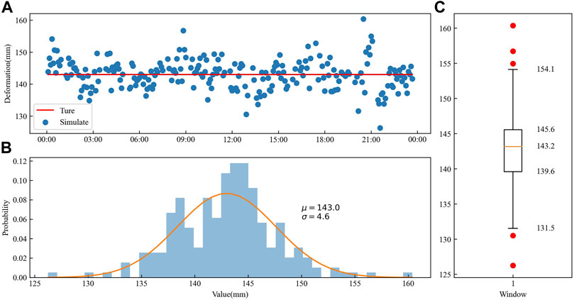
FIGURE 3. Situation one simulation signal and estimation result. (A) Simulated deformation scatters plot and true value; (B) Frequency distribution histogram and probability distribution curve; (C) Boxplot of window sample.

Situation 2: Based on the original signal, three outliers (200, 180, and 300) were added at times of 08:20:00, 14:50:00, and 20:35:00. Because the outliers did not affect the true deformation of the window, it remained unchanged at 143.0 mm (Figure 4A).

FIGURE 4

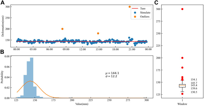
FIGURE 4. Situation two simulation signal and estimation result. (A) Simulated deformation scatters plot and true value; (B) Frequency distribution histogram and probability distribution curve; (C) Boxplot of window sample.

Situation 3: Simulated deformation was added to the original signal. Referring to the existing landslide failure data, the initial rate and acceleration of deformation were set at 2.4 mm/h and 0.024 mm/h². The true deformation at the center of the window (12:00:00) was 193.0 mm (Figure 5A).

FIGURE 5

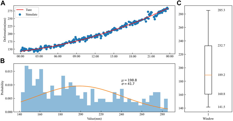
FIGURE 5. Situation three simulation signal and estimation result. (A) Simulated deformation scatters plot and true value; (B) Frequency distribution histogram and probability distribution curve; (C) Boxplot of window sample.

Situation 4: Based on the simulated deformation, the window width was reduced to 4 h, and the true deformation at the center of the window (12:00:00) was still 193.0 mm (Figure 6A).

FIGURE 6

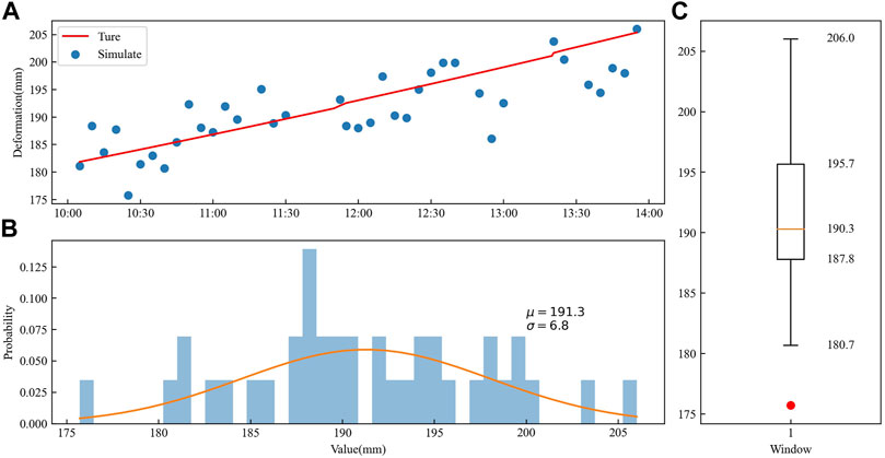
FIGURE 6. Situation four simulation signal and estimation result. (A) Simulated deformation scatters plot and true value; (B) Frequency distribution histogram and probability distribution curve; (C) Boxplot of window sample.

The frequency distribution histogram of situation 1 (Figure 3B) showed a normal distribution. The outliers were evenly distributed on both sides of the boxplot (Figure 3C), indicating that both methods yield optimal estimation results. A comparison with the conventional estimators and the NIQR estimators showed that the NIQR estimation was similar to that of conventional methods (Table 1).

TABLE 1

TABLE 1. Estimated results of the four simulated deformations.

When the outliers were added to the original signal (situation 2), the frequency distribution was asymmetrical, the peak was off-center toward the left, and the tail stretched away from the peak (Figure 4B). The boxplot successfully excluded these outliers (Figure 4C). Because it is affected by outliers, the conventional estimation method is quite different from that of situation 1, and the NIQR estimators showed little change. Therefore, the NIQR estimation method is robust.

When the simulated deformation was added to the original signal (situation 3), the series showed a gradually increasing trend, and the histogram shapes exhibited a right-skewed distribution (Figure 5B). The upper half of the boxplot was higher than the lower half (Figure 5C), and both halves showed large deviations that did not reflect the true deformation of the window because of the existence of the breakdown point.

Situation 4 reduced the window width and weakened the skewness of the frequency distribution histogram (Figure 6B) and window sample boxplot (Figure 6C). The NIQR estimated results were similar to the results obtained without simulated deformation; therefore, deformation in the window can be ignored.

4 Results

4.1 Study Area

Heifangtai is a loess tableland located 60 km west of Lanzhou City in Gansu province, China. As this terrace was converted to agricultural land in 1968, excessive agricultural irrigation has induced more than 200 loess landslides and caused almost 40 casualties (Bai et al., 2019; Kong et al., 2021). A loess landslide (DC#5 landslide, 36°5′30.93″N, 103°18′43.6″E) occurred at 13:00 (UTC) on 27 January 2021, in the Heifangtai terrace (Figure 7A). Fortunately, the “High Precision Beidou System for Landslide Hazard Monitoring and Early Warning,” developed at Chang’an University (China), successfully recorded the entire cumulative displacement–time data in real-time (Figures 7B,C). The data source for this article comes from this system. The GNSS processing software is developed by Chang’a University. The BDS/GPS relative positioning solution uses a partially ambiguity fixing method based on the data collected by the GNSS monitor station. The satellite cut-off height is 10°, and the ephemeris uses the broadcast ephemeris (Huang et al., 2018; Bai et al., 2019).

FIGURE 7

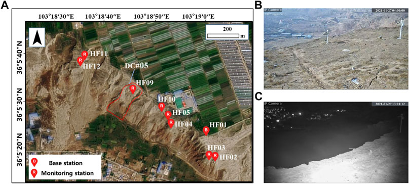
FIGURE 7. (A) Layout of the global navigation satellite system monitoring systems at Heifangtai. And the location of DC#5 landslide occurred on 17 January 2021; (B) Photo of the HF09 monitoring station located at DC#5 before the landslide event; (C) Photo of the HF09 monitoring station after the landslide event.

The raw GNSS displacement time series of the HF09 monitoring station located at DC#5 is presented in Figure 8, where R is the square root of displacements in the east (E), north (N), and upward (U) directions. The GNSS displacement time series is a typical three-stage creep curve but shows many outliers, large random noise, and inconsistent data intervals, creating difficulties in the calculation of the warning criteria. Further preprocessing of the series is required to extract accurate deformation

FIGURE 8

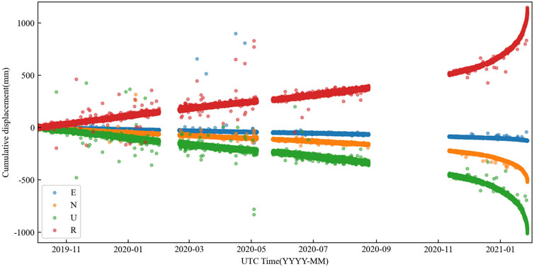
FIGURE 8. Raw GNSS displacement time series of the HF09 monitoring station of the GNSS monitoring systems. They include east (E), north (N), upward (U), and three-dimensional (R) directions.

4.2 Fixed Width Sliding-Window Estimation Results

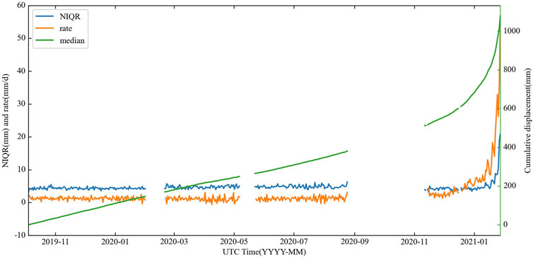
A fixed window width of 24 h was used to segment the GNSS displacement time series, and the window sample was estimated by calculating the median and NIQR. Simultaneously, the deformation rate between windows can be easily calculated, as shown in Figure 9. The deformation rate is relatively small in steady-state creep; thus, the GNSS positioning error is the main component of the window error, preventing the NIQR statistics from changing over time. The deformation rate tends to increase after the accelerating creep stage is reached, resulting in a gradually increasing proportion of outliers in the window. The NIQR estimators also began to rise sharply until their proportion reached a breakdown point, after which the median and NIQR estimators no longer represent the true deformation feature of the window.

FIGURE 9

FIGURE 9. Fixed width sliding-window estimation results and deformation rate.

4.3 Adaptive Sliding-Window Deformation Feature Results

According to the processing flow described in Section 2.4, the adaptive sliding window method was used to preprocess the monitoring series in the accelerating creep stage (10 November 2020 to 27 January 2021). Windows with no obvious outliers were selected from November 15, 2020 to December 15, 2020, and a width adjustment strategy was used to shorten the width by half each time until the width was less than 1 h to use real-time results. The key parameters in the adaptive sliding window method are listed in Table 2 and are shown in Figure 10. The window coefficients were adjusted five times, and each adjustment caused the breakdown point to reach the same deformation rate later. This result verifies that adjusting the window coefficients can effectively reduce the number of outliers.

TABLE 2

TABLE 2. Key parameters in the process of the adaptive sliding-window method.

FIGURE 10

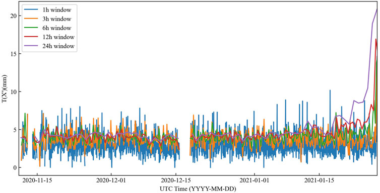
FIGURE 10. Estimated normalized interquartile ranges of the window sample used as $T\left(X\text{'}\right)$ to calculate bias in the adaptive sliding-window method.

Figure 11 shows the deformation feature results obtained using the adaptive sliding window method after processing. Compared to the raw GNSS displacement time series, the time series after feature extraction more accurately described the creep curve during the accelerated creep stage.

FIGURE 11

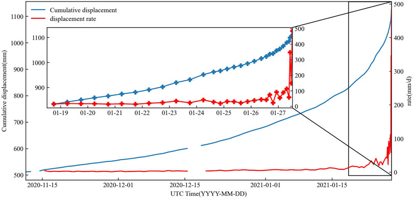
FIGURE 11. Time series of the cumulative displacement estimation result and deformation rate of the adaptive sliding-window.

4.4 Application of DC#5 Loess Landslides Early Warning

Based on the ability of the threshold definition method to suggest a probable failure, the adaptive sliding window method successfully assisted in the early warning of the DC#5 loess landslide. According to the creep curve of the loess slopes and previous findings in the Heifangtai area (Xu et al., 2020), a five-level alert criterion for the deformation rate threshold can be defined, as shown in Table 3. This alert was published by the local government. After receiving the warning information, the involved departments immediately launched an emergency response to evacuate people in the zone affected by the landslide. Because of this early warning, no casualties or property damage occurred.

TABLE 3

TABLE 3. Key parameters in the process of the adaptive sliding-window method.

5 Discussion

To address the problem of the relationship between noise and true deformation changes in different creep stages, we proposed an adaptive sliding-window method for accurately extracting deformation features. Simulation experiments were conducted to evaluate the performance of the sliding window approach for different outliers and deformation signals.

According to the simulation results in the four situations, when the window sample contained only random noise, the NIQR estimation was equivalent to that of conventional methods. The NIQR estimation method is robust in the presence of outliers in the window sample. When window deformation occurred, both estimation methods reached their breakdown point, and the performance decreased. Reducing the width of the window can overcome this problem when the estimation method reaches the breakdown point.

A series of experiments were performed in the Heifangtai area to assess the practical application of the proposed method. The results for the time series of the cumulative displacement estimation of the adaptive sliding window showed that this method effectively reduces random noise and outliers and more accurately describes the creeping trend of the landslide. The window was used to extract the creep feature rather than a large number of unnecessary observations, which is convenient for further data analysis. Additionally, since the algorithm only works on the estimation of a single window, data interruptions have less impact on feature extraction.

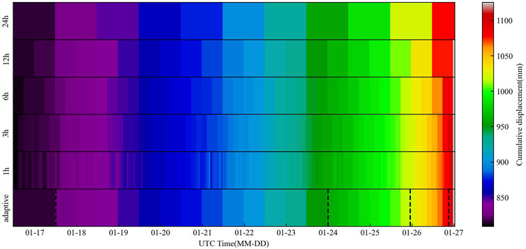
Figure 12 shows a comparison of the fixed sliding window and adaptive sliding window, where the different colored blocks represent different windows and the color represents the estimated value of cumulative displacement. The window coefficient is adjusted by the black line in the figure.

FIGURE 12

FIGURE 12. Cumulative displacement colormap of partial adaptive sliding-window estimation results.

In the first half of the color map, when the deformation rate was small, the deformation feature extraction results with a wider window were smoother and more reliable. Although the window lag was larger, the estimated results were close to the actual values within the window range because of the smaller deformation rate; therefore, window lag can be ignored. However, the deformation feature extraction results obtained with a shorter window showed that cumulative displacement decreased, which affected subsequent deformation analysis.

As the deformation rate increases, the lag of the window must be considered. Therefore, a shorter window width can represent a more realistic deformation feature. Our adaptive sliding-window method combines the characteristics of a wide window and a short window in different creep stages, ensuring the reliability and real-time performance of the deformation feature extraction results.

In summary, the proposed algorithm showed high reliability and practicality for obtaining creep curves and may provide support for landslide early warning. The results of the adaptive sliding-window method constantly change, which may limit the early warning method. Further studies are necessary to consider early warning methods that are more suitable for variable interval data to achieve better performance.

6 Conclusion

Landslide monitoring and early warnings are important in the study of landslide hazards. To obtain more accurate deformation features, raw monitoring results must be preprocessed. However, at different creep stages, the relationship between noise and deformation changes, potentially resulting in constant changes in the covariance of the dataset. This study presents an adaptive sliding-window algorithm based on the concept of the sample breakdown point.

The sliding window method is a simple and adaptable preprocessing approach for landslide monitoring. This method accurately extracts the deformation features of the window by estimating the window sample, thereby effectively reducing the influence of random noise and outliers on the results.

As the deformation rate increases, the window may reach a breakdown point. To overcome this limitation, a method based on the definition of the prior breakdown point is proposed for determining the breakdown point. The breakdown point can be postponed by adjusting the window parameters.

The processing results of the real GNSS landslide monitoring series showed that the proposed algorithm can provide reliable deformation information for landslide warnings even if the landslide is undergoing imminent failure. This algorithm could be selected as a useful reference for preprocessing methods and early warning for landslide monitoring series.

Data Availability Statement

The original contributions presented in the study are included in the article/Supplementary Material, further inquiries can be directed to the corresponding author.

Author Contributions

GH and DW designed the processing strategy and experiments, performed the experimental analyses, and wrote the manuscript. DW and YD contributed to the collection and analysis of field test data. QZ, ZB, and CW helped improve the manuscript.

Funding

This work was financially supported by the National Key Research and Development Plan of China (2018YFC1505105) and Program of the National Natural Science Foundation of China (42090053, 42127802, and 41941019).

Conflict of Interest

The authors declare that the research was conducted in the absence of any commercial or financial relationships that could be construed as a potential conflict of interest.

Publisher’s Note

All claims expressed in this article are solely those of the authors and do not necessarily represent those of their affiliated organizations, or those of the publisher, the editors, and the reviewers. Any product that may be evaluated in this article, or any claim that may be made by its manufacturer, is not guaranteed or endorsed by the publisher.

Acknowledgments

The authors would like to thank the reviewers and the editors for their constructive comments on this manuscript.

References

Amiri-Simkooei, A. R. (2008). Noise in Multivariate GPS Position Time-Series. J. Geod 83 (2), 175–187. doi:10.1007/s00190-008-0251-8

CrossRef Full Text | Google Scholar

Bai, Z., Zhang, Q., Huang, G., Jing, C., and Wang, J. (2019). Real-time BeiDou Landslide Monitoring Technology of "light Terminal Plus Industry Cloud. Acta Geodaetica et Cartographica Sinica 48, 1424–1429.

Google Scholar

Banerjee, P., and Bansal, S. (2017). Revisit of Moving Average Technique for Smoothing GNSS Based Timing Data. Mapan 32 (1), 77–85. doi:10.1007/s12647-016-0200-6

CrossRef Full Text | Google Scholar

Benoit, L., Briole, P., Martin, O., and Thom, C. (2014). Real-time Deformation Monitoring by a Wireless Network of Low-Cost GPS. J. Appl. Geodesy 8 (2). doi:10.1515/jag-2013-0023

CrossRef Full Text | Google Scholar

Buch, K. D. (2014). “Decision Based Non-linear Filtering Using Interquartile Range Estimator for Gaussian Signals,” in 2014 Annual IEEE India Conference (INDICON) (IEEE), 1–5. doi:10.1109/indicon.2014.7030658()

CrossRef Full Text | Google Scholar

Dok, A., Fukuoka, H., Katsumi, T., and Inui, T. (2011). Tertiary Creep Reproduction in Back-Pressure-Controlled Ring Shear Test to Understand the Mechanism and Final Failure Time of Rainfall-Induced Landslides. Kyoto Univ. Disaster Prev. Res. Inst. Annu. Rep. 54, 263–270.

Google Scholar

Donoho, D. L., and Huber, P. J. (1983). The Notion of Breakdown Point. in A Festschrift for Erich L Lehmann.

Google Scholar

Du, Y., Huang, G., Zhang, Q., Gao, Y., and Gao, Y. (2020). Asynchronous RTK Method for Detecting the Stability of the Reference Station in GNSS Deformation Monitoring. Sensors 20 (5), 1320. doi:10.3390/s20051320

PubMed Abstract | CrossRef Full Text | Google Scholar

Foster, J., Bevis, M., and Businger, S. (2005). GPS Meteorology: Sliding-Window Analysis*. J. Atmos. Oceanic Technology 22 (6), 687–695. doi:10.1175/jtech1717.1

CrossRef Full Text | Google Scholar

Fried, R., and Gather, U. (2007). On Rank Tests for Shift Detection in Time Series. Comput. Stat. Data Anal. 52 (1), 221–233. doi:10.1016/j.csda.2006.12.017

CrossRef Full Text | Google Scholar

Froude, M. J., and Petley, D. N. (2018). Global Fatal Landslide Occurrence from 2004 to 2016. Nat. Hazards Earth Syst. Sci. 18 (8), 2161–2181. doi:10.5194/nhess-18-2161-2018

CrossRef Full Text | Google Scholar

Han, J., Huang, G., Zhang, Q., Tu, R., Du, Y., and Wang, X. (2018). A New Azimuth-dependent Elevation Weight (ADEW) Model for Real-Time Deformation Monitoring in Complex Environment by Multi-GNSS. Sensors 18 (8), 2473. doi:10.3390/s18082473

PubMed Abstract | CrossRef Full Text | Google Scholar

Huang, G., Huang, G., Du, Y., Tu, R., Han, J., and Wan, L. (2018). A Lowcost Real-Time Monitoring System for Landslide Deformaion with Beidou Cloud. J. Eng. Geology. 26 (4), 1008–1016.

Google Scholar

Peter, J. Huber, and Elvezio, M. Ronchetti (2009). Robust Statistics. 2nd ed. John Wiley & Sons

Google Scholar

Ince, C. D., and Sahin, M. (2000). Real-time Deformation Monitoring with GPS and Kalman Filter. Earth Planet. Sp 52 (10), 837–840. doi:10.1186/BF03352291

CrossRef Full Text | Google Scholar

Intrieri, E., Carlà, T., and Gigli, G. (2019). Forecasting the Time of Failure of Landslides at Slope-Scale: A Literature Review. Earth-Science Rev. 193, 333–349. doi:10.1016/j.earscirev.2019.03.019

CrossRef Full Text | Google Scholar

Ismail, Z., Efendi, R., and Deris, M. M. (2013). Inter-quartile Range Approach to Length-Interval Adjustment of Enrollment Data in Fuzzy Time Series Forecasting. Int. J. Comp. Intel. Appl. 12 (03), 1350016. doi:10.1142/s1469026813500168

CrossRef Full Text | Google Scholar

Kong, J.-x., Zhuang, J.-q., Zhan, J.-w., Bai, Z.-w., Leng, Y.-q., Ma, P.-h., et al. (2021). A Landslide in Heifangtai, Northwest of the Chinese Loess Plateau: Triggered Factors, Movement Characteristics, and Failure Mechanism. Landslides 18 (10), 3407–3419. doi:10.1007/s10346-021-01752-z

CrossRef Full Text | Google Scholar

Li, G., Dai, W., and Zeng, F. (2016). Robust Moving Average in GPS Automatic Monitoring Data Processing Applications. J. Geodesy Geodyn 36 (1), 85–88.

Google Scholar

Li, L., and Kuhlmann, H. (2013). Real-time Deformation Measurements Using Time Series of GPS Coordinates Processed by Kalman Filter with Shaping Filter. Surv. Rev. 44 (326), 189–197. doi:10.1179/1752270611y.0000000022

CrossRef Full Text | Google Scholar

Ren, L., and Xu, T.-H. (2018). “Research on Smoothing Filtering Algorithm of BDS/GPS Slow Deformation Monitoring Sequence,” in China Satellite Navigation Conference (CSNC) 2018 Proceedings, 33–44. doi:10.1007/978-981-13-0005-9_3

CrossRef Full Text | Google Scholar

Schmitt, E., Öllerer, V., and Vakili, K. (2014). The Finite Sample Breakdown point of PCS. Stat. Probab. Lett. 94, 214–220. doi:10.1016/j.spl.2014.07.026

CrossRef Full Text | Google Scholar

Song, H. Y., and Lee, J. S. (2015). Detecting Positioning Errors and Estimating Correct Positions by Moving Window. PLoS One 10 (12), e0143618. doi:10.1371/journal.pone.0143618

PubMed Abstract | CrossRef Full Text | Google Scholar

Tavenas, F., and Leroueil, S. (1981). Creep and Failure of Slopes in Clays. Can. Geotech. J. 18 (1), 106–120. doi:10.1139/t81-010

CrossRef Full Text | Google Scholar

Xu, Q., Peng, D., Zhang, S., Zhu, X., He, C., Qi, X., et al. (2020). Successful Implementations of a Real-Time and Intelligent Early Warning System for Loess Landslides on the Heifangtai Terrace, China. Eng. Geology. 278, 105817. doi:10.1016/j.enggeo.2020.105817

CrossRef Full Text | Google Scholar

Xu, Q., Yuan, Y., Zeng, Y., and Hack, R. (2011). Some New Pre-warning Criteria for Creep Slope Failure. Sci. China Technol. Sci. 54 (S1), 210–220. doi:10.1007/s11431-011-4640-5

CrossRef Full Text | Google Scholar

Yang, Y. M., Wang, Z. G., Gao, Y. Y., and Gao, F. P. (2012). Deformation Monitoring Data De-noising Processing Based on Wavelet Packet. Amm 166-169, 1180–1186. doi:10.4028/www.scientific.net/AMM.166-169.1180

CrossRef Full Text | Google Scholar

Zhao, L., Qiu, H., and Feng, Y. (2016). Analysis of a Robust Kalman Filter in Loosely Coupled GPS/INS Navigation System. Measurement 80, 138–147. doi:10.1016/j.measurement.2015.11.008

CrossRef Full Text | Google Scholar

Zhu, X., Xu, Q., Qi, X., and Liu, H. (2017). “A Self-Adaptive Data Acquisition Technique and its Application in Landslide Monitoring,” in Advancing Culture of Living with Landslides, 71–78. doi:10.1007/978-3-319-53487-9_7

CrossRef Full Text | Google Scholar