Study on the Calculation Method of Active Earth Pressure and Critical Width for Finite Soil Behind the Retaining Wall

The method to determine the active earth pressure and critical width for finite soil behind the retaining wall in mountainous areas is one of the concerns of geotechnical engineering. In order to study the active earth pressure distribution of the finite soil against the retaining wall and determine the critical width of the boundary between the finite soil and the semi-infinite soil, this study focuses on investigating a retaining wall with finite cohesionless backfill. The shape of the failure surface is assumed to be a cycloid passing through the heel of the wall in the limit equilibrium state. Considering the deflection of soil principal stress induced by wall–soil friction effect, a calculation method of active earth pressure for finite soil is proposed by using an arc-shaped small principal stress trajectory, and the rationality of this method is verified. On this basis, a calculation formula of the critical width for finite soil is proposed. The influence of the internal friction angle and the wall–soil friction angle on the critical width of finite soil is examined. The results indicate that the active earth pressure of finite soil presents a nonlinear drum distribution along the height of the retaining wall under the failure mode of the cycloidal surface. The maximum value of active earth pressure is close to the bottom of the wall. The critical width of finite soil decreases with the increase of the internal friction angle, and its variation rate decreases gradually. The critical width of finite soil increases with the increase of the wall–soil friction angle, and its variation rate also increases gradually. Under different internal friction angles and wall–soil friction angles, the critical width values of finite soil calculated by the assumption of the cycloidal failure surface are smaller than those calculated by the Coulomb earth pressure calculation method.

Introduction

At present, the classical earth pressure theory is widely used to calculate earth pressure in the design of retaining walls, and one of the prerequisites is that the soil behind the wall is a semi-infinite space body. In mountain road engineering, due to the influence of geology, topography, and boundary line of the land, many retaining walls are close to the stable rock strata, and a large number of foundation pits in the cities are also close to the buildings (Huang et al., 2021; Huang et al., 2022). Under the aforementioned scenarios, the soil behind the wall should be considered finite, and the boundary conditions and failure modes are obviously different from the semi-infinite soil. Furthermore, the basic assumption of classical earth pressure theory is that the slip surface behind the wall is a plane surface, but a large number of model tests and practical projects have proved that the slip surface should be curved (Liu et al., 2021; Huang et al., 2021). The reasonable value of soil pressure is an important basis for the design of retaining walls. If the classical soil pressure theory is still used to calculate the size and distribution of active soil pressure of finite soil, it will inevitably increase the error of the design, which may affect the safety of structures in serious cases. Therefore, it is necessary to determine the critical width of finite soil and subsequently seek a method to calculate the active earth pressure of finite soil.

Several scholars have studied the soil pressure of finite soil in various aspects. Wang et al. (2016) derived the expression of soil pressure of non-cohesive finite soil by using the horizontal thin-layer element method. The results illustrated that the ultimate failure angle of finite soil varied with the parameters. Hu et al. (2018) derived the soil pressure calculation method of finite width soil under limit state based on the plastic upper limit theory of soil, considering the frictional energy consumption between the retaining wall and the building–soil interface. Handy (1985) derived the soil pressure distribution curve behind the wall by assuming a suspended chain linear principal stress trajectory line between two parallel walls. The shape of the principal stress trajectory to arc curve was simplified to derive the calculation formula of active earth pressure of a rigid retaining wall by assuming the retaining wall surface and the sliding surface as two arch feet in Rankine’s theory (Paik and Salgado, 2003). Liu (2018) considered the shear stress between the horizontal soil layers in the sliding soil wedge behind the wall. The horizontal differential layer method was applied to analyze the stress. Meanwhile, the equilibrium control equation was established, and the theoretical expression of active earth pressure with nonlinear distribution was obtained. Zhao and Zhu (2014) solved the lateral earth pressure coefficients based on the principal stress rotation concept, from which the active earth pressure solutions for finite soils were derived. Xu et al. (2019) derived the distribution of soil pressure by assuming the minor principal stress trajectory as circular, catenary, and parabola. Xu et al. (2020) studied a finite range of cohesive soils behind the retaining wall and obtained the theoretical expression of active earth pressure for finite soil, considering the soil arching effects. The distribution law of lateral earth pressure on the wall side of the retaining wall under the active translation mode was investigated by the model test, and the arch effect behind the retaining wall under the active translation mode was verified (Khosravi et al., 2013). The soil arching effect was considered to calculate the finite soil pressure between two parallel retaining walls with cohesive fill. The results indicated that the earth pressure without considering the soil arch effect is on the dangerous side according to the conventional method (Wu et al., 2014).

The aforementioned studies assume that the failure mode of soil is a linear failure, and the results of multiple model tests show that the slip surface of soil behind the wall is curved (Yang et al., 2016; He et al., 2020). He et al. (2020) studied the development laws of displacement and shear strain in the process of active failure of soil using particle image velocimetry technology and translational model tests of rigid retaining walls with different aspect ratios. According to the test results, the final soil sliding surface is composed of two parts: the plane presented π/4+φ/2 with the horizontal plane in the range of 0.815–1.0 H and the sliding surface in the range of 0–0.815 H, which is a surface between the Coulomb sliding surface and the logarithmic spiral. An experimental study on the soil pressure for finite width non-cohesive soil behind a rigid retaining wall was carried out (Yang et al., 2016). The results show that the failure surface of the soil with finite width is a continuous surface. Cao (1995) studied the distribution of soil pressure behind the retaining wall by assuming the generation of a cycloidal failure surface in the semi-infinite soil. Yang et al. (2017) assumed the sliding surface of semi-infinite soil as a cycloidal line to study the soil pressure distribution behind the retaining wall by considering the soil arching effect. The slip surface curve of the semi-infinite soil behind the wall with a vertical back and horizontal surface was proposed as a logarithmic spiral under the limit state. The corresponding active earth pressure calculation formulas were also derived (Wang et al., 2011). Greco. (2013) studied a finite width retaining wall with non-cohesive soil fill. The failure mode of multi-line soil was proposed, and the finite width soil pressure was calculated by the limit equilibrium method. The slip surface curve of the finite soil behind the wall was considered a logarithmic spiral, and the corresponding active earth pressure calculation formula was proposed (Yang et al., 2017; Yang et al., 2020). However, the theoretical fracture angle was not given. The results found that the initial fracture angle of the finite soil slip surface with different width-to-height ratios could be taken as π/4+φ/2 with partial safety.

From the aforementioned studies, it can be concluded that when the soil behind the wall is finite, the calculation of soil pressure by using the curve slip surface is more in line with the actual situation. Therefore, in order to calculate the distribution of active earth pressure of finite soil more reasonably and explore the value of the critical width between finite soil and semi-infinite soil, this article assumes that the sliding surface of the soil is a cycloidal line, considering the influence of principal stress deflection of soil. The function expression of the sliding surface of the cycloidal line and the critical width of finite soil is obtained by calculation. Meanwhile, the corresponding calculation method of active earth pressure of finite soil is proposed. The influence of the internal friction angle and wall–soil friction angle of finite width soil on the critical width of finite soil is discussed in depth, which can provide design reference for the retaining wall design of related projects in the future.

Theoretical Analysis of Active Earth Pressure

Mechanical Model of Earth Pressure

As shown in Figure 1, a schematic diagram is established with finite soil as the research object, with the retaining wall on the left, the bedrock on the right, and non-cohesive soil between them. The width of the finite soil is X. The internal friction angle of the soil is $\varphi$. The gravity is $\gamma$. The buried depth of the retaining wall is Z₁. The external friction angle of the soil is ${\delta }_1$. The distance between the intersection of the bedrock and sliding surface and the ground is Z₂. The external friction angle of the soil is ${\delta }_2$. When the soil reaches the limit equilibrium state, a curve slip surface through the bottom of the wall is formed within the soil. H is the height of the slip surface. $\psi$ is the angle between the tangent of any point of the slip line and the horizontal line. According to the different boundary conditions, the finite soil is divided into I and II zones.

FIGURE 1

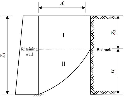
FIGURE 1. Mechanical model of earth pressure.

The following assumptions are made to simplify the theoretical derivation:

1) The finite soil behind the wall is a single soil layer, which is homogeneous and non-cohesive.

2) It is assumed that the supporting structure only moves in the plane, and each section of the supporting structure remains a complete plane along the transverse direction, which is perpendicular to the longitudinal direction.

3) Ignore the effect of the supporting structure weight.

4) The slip surface passes through the bottom of the retaining wall structure.

Assumption of the Soil Sliding Surface

If the classical earth pressure theory is used to calculate the active earth pressure, one of its assumptions is that the sliding surface is a straight line passing through the bottom of the wall. However, the experiments and theories of some scholars proved that the sliding surface of active earth pressure is not a straight line. A number of nonlinear sliding surface models have been proposed by many scholars, such as cycloidal lines (Cao, 1995; Yang et al., 2017), logarithmic spiral curves (Wang et al., 2011; He et al., 2020), and folding lines (Greco, 2013). In this study, it is assumed that when the retaining wall is in limit equilibrium, the soil in the active zone behind the wall produces a cycloidal line slip surface through the heel of the wall as shown in Figure 2.

FIGURE 2

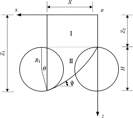
FIGURE 2. Cycloidal failure surface.

The right-angle coordinate system is established as shown in Figure 2. The equation of the cycloidal line can be expressed as:

$\{\begin{array}{l}x=R_1(\theta -\sin \theta );\\ z=R_1(1-\cos \theta )+Z_2,\end{array}(1)$

where R₁ is the radius of the rotating wheel, and θ is the rotating angle.

When the cycloidal line passes through the wall toe, $z=Z_1$, the radius of the rotating wheel can be obtained as:

$R_1=\frac{X}{{\theta }_c-\sin {\theta }_c},(2)$

where ${\theta }_{\text{c}}$ is the initial rotating angle of the cycloidal line.

Thus, the height of the cycloidal line slip surface can be obtained as Eq. 3:

$H=Z_1-Z_2=R_1(1-\cos {\theta }_c),(3)$

If $H\ge Z_1$, it indicates that the sliding surface of soil reaches the ground within the range of finite soil, which is semi-infinite at this time. Take $Z_2=0$, then R₁ is calculated by the second equation in Eq. 4:

$R_1=\frac{Z_1}{1-\cos {\theta }_c},(4)$

The rotating angle θ at any point on the slip surface is shown as:

$\theta =\arccos (1-\frac{z-Z_2}{R_1}),(5)$

The slope of any point on the slip surface tanψ is shown in Eq. 6:

$\tan \psi =\frac{dz}{dx}=\tan (\frac{\pi }{2}-\frac{\theta }{2}),(6)$

The angle between the tangent and horizontal direction at any point on the slip surface ψ is shown as:

$\psi =\frac{\pi }{2}-\frac{\theta }{2},(7)$

Stress Analysis of Soil

With the lateral displacement of the retaining wall during the active failure of the soil, the soil and the back of the wall produce relative slip. The friction between the wall and the soil deflects principal stress of the soil element. After the soil element is deflected, the curve formed by the principal stress direction is called the principal stress trajectory. The principal stress trajectory is generally a catenary curve. Paik and Salgado (2003) compared the catenary trajectory line with the arc trajectory line. The results show that the difference between the two calculation results is not significant. Meanwhile, the circular arc is simpler than the catenary calculation, which is more convenient for practical application. Therefore, this study adopts the circular arc for stress analysis.

Layer AB of Zone I is shown in Figure 3, and layer AB of Zone II is shown in Figure 4. The length is L_z. When the soil after the retaining wall reaches the active limit equilibrium state, the stress deflection occurs in AB, which forms a circular arc minor principal stress trajectory. The center of the circle is located at point O in the figure. The radius is R₂. The angle between the connection line of any point D in the arc and the center O in the horizontal direction is ε. The angle between AO and the horizontal direction is ε_A. The angle between BO and the horizontal direction is ε_B.

FIGURE 3

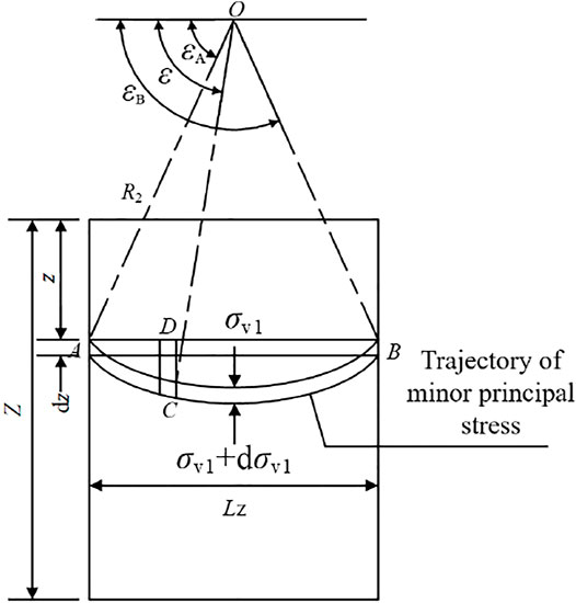
FIGURE 3. Trajectory of minor principal stress of Zone I

FIGURE 4

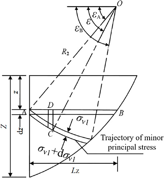
FIGURE 4. Trajectory of minor principal stress of Zone II

When active failure occurs at point D, the horizontal ${\sigma }_h$ and vertical stresses ${\sigma }_v$ can be expressed as (Zhu and Zhao, 2014):

$\{\begin{array}{l}\frac{{\sigma }_v}{{\sigma }_1}={{\displaystyle \sin }}^2\omega +K_a{{\displaystyle \cos }}^2\omega ;\\ \frac{{\sigma }_h}{{\sigma }_1}={{\displaystyle \cos }}^2\omega +K_a{{\displaystyle \sin }}^2\omega ;\end{array}(8)$

$K_a={\sigma }_3\text{/}{\sigma }_1=(1-\sin \phi )/(\text{1}+\sin \phi ),(9)$

where $\omega$ is the angle between major principal stress and horizontal direction.

The vertical force of point D, i.e., $\text{d}V$ is shown as:

$\text{d}V={\sigma }_{V}dA=\frac{{\sigma }_1\left[1-\cos \left(2\omega \right)\sin \phi \right]}{1+\sin \phi }{R}_2\sin \omega d\omega .(10)$

The relationship between the radius of small principal stress traces R₂ and the distance L_z between the two points AB is as follows:

$R_2=L_z\text{/}(\cos {\epsilon }_B-\cos {\epsilon }_A),(11)$

It can be seen from Figure 5 that the angle between the minor principal stress at point A and the horizontal direction is ε_A. The angle between the minor principal stress at point B and the right tangent is ε_B.

FIGURE 5

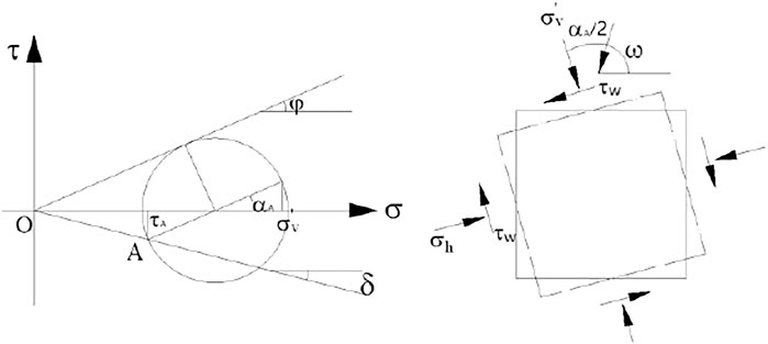
FIGURE 5. Mohr’s circle of stress at point A.

When AB is located in Zone I:

${\epsilon }_A=\pi \text{/}2-{\alpha }_{\text{A}}\text{/}2\text{,}(12)$

${\alpha }_{\text{A}}=\text{arc}\sin \left(\frac{\sin {\delta }_1}{\sin \phi }\right)-{\delta }_1,(13)$

${\epsilon }_B=\pi \text{/}2+{\alpha }_B/2,(14)$

${\alpha }_B=\text{arc}\sin \left(\frac{\sin {\delta }_1}{\sin \phi }\right)-{\delta }_2,(15)$

When AB is located in Zone II:

ε_A is the same as in Zone I, ε_B is equal to the sum of the angle between the minor principal stress at point B and the tangential direction of the slip surface, and the angle between the tangential direction of the slip surface and the horizontal direction, namely,

${\epsilon }_B=\pi \text{/}4-\phi /2+\psi ,(16)$

In the calculation of earth pressure on retaining walls by the horizontal differential layer method, the active lateral earth pressure coefficient $K_{awn}$ is the ratio between ${\sigma }_h$ and vertical average stress $\overline{{\sigma }_v}$.

The following equation can be deduced:

$K_{awn}=\frac{{\sigma }_h}{\overline{{\sigma }_v}}=\frac{{\sigma }_1({\cos }^2{\epsilon }_A+K_a{\sin }^2{\epsilon }_A)}{\frac{{\displaystyle {\int }_{l_{AB}}dV}}{L_z}}=\frac{{\cos }^2{\epsilon }_A+K_a{\sin }^2{\epsilon }_A}{1+\frac{\left({\cos }^3{\epsilon }_A-{\cos }^3{\epsilon }_B\right)\left(K_a-1\right)}{3\left(\cos {\epsilon }_A-\cos {\epsilon }_B\right)}},(17)$

It can be seen from Eq. 17 that when the horizontal differential layer is located in Zone I, $K_{awn}$ is a fixed value; when the horizontal differential layer is located in Zone II, it changes with the slope of the slip line, namely, $K_{awn}$ changes with the rotation angle of the cycloidal line.

Calculation of Active Earth Pressure

A horizontal differential element layer at z from the ground is taken, and the equilibrium equations are established for analysis according to the different stresses on the soil in Zone I and Zone II. Assuming that there is no relative slip between the horizontal differential layers of soil, namely, the shear stress between layers is not considered.

The mechanical model is shown in Figure 6 when the horizontal differential layer is located in the soil of Zone I, $z<Z_2$. ${\sigma }_{v1}$ is the average vertical stress acting on the upper surface of the differential element, ${\sigma }_{v1}+d{\sigma }_{v1}$ is the average vertical stress acting on the lower surface, ${\sigma }_{h1}$ is the horizontal stress of the retaining wall structure side, and ${\sigma }_n$ is the horizontal stress of the bedrock side. The thickness of the differential horizontal element is $dz$, and the volume is $dV$.

FIGURE 6

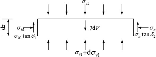
FIGURE 6. Microelement mechanical model of Zone I.

According to the balance of forces in the horizontal direction, Eq. 18 can be obtained:

${\sigma }_{h1}dz-{\sigma }_{n}dz=\mathrm{0,}(18)$

According to the balance of stresses in the vertical direction, Eq. 19 can be obtained:

$X\text{d}{\sigma }_{v1}+{\sigma }_{h1}\tan {\delta }_{1}dz+{\sigma }_n\tan {\delta }_2\text{dz}=\gamma \text{d}V,(19)$

Combining Eqs 17–19:

$X\text{d}{\sigma }_{v1}+K_{awn}{\sigma }_{v1}\tan {\delta }_{1}dz+K_{awn}{\sigma }_{v1}\tan {\delta }_2\text{dz}=X\gamma \text{d}z.(20)$

Differential Eq. 21 can be obtained:

$\frac{\text{d}{\sigma }_{v1}}{\text{dz}}=\gamma -\frac{K_{awn}{\sigma }_{v1}(\tan {\delta }_1+\tan {\delta }_2)}{X}.(21)$

The horizontal earth pressure is:

${\sigma }_{h1}=K_{awn}{\sigma }_{v1},(22)$

When the horizontal differential layer is located in Zone II, $Z_2<z<Z_1$. The mechanical model is shown in Figure 7. ${\sigma }_{v2}$ is the average vertical stress acting on the upper surface of the differential element. ${\sigma }_{v2}+d{\sigma }_{v2}$ is the average vertical stress acting on the lower surface. ${\sigma }_{h2}$ is the horizontal stress acting on the side of the retaining wall. $r$ is the reaction of soil to the differential element. $\phi$ is the internal friction angle of the soil. $\psi$ is the angle between the tangent of the slip surface at the differential unit and the horizontal direction. The thickness of the differential unit is $dz$. The volume is $dV$.

FIGURE 7

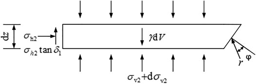
FIGURE 7. Microelement mechanical model of Zone II.

The top width of the differential element can be calculated as:

$B_1=X(1-\frac{\theta -\text{sin}\theta }{{\theta }_c-\sin {\theta }_c}).(23)$

The bottom width of the microelement can be calculated as:

$B_2=B_1-\cot \psi dz=B_1-\tan \frac{\theta }{2}dz,(24)$

The microelement weight can be calculated as:

$\gamma dV=\frac{\gamma }{2}(B_1+B_2)dz,(25)$

Omitting the higher order differential, we get:

$\gamma dV=\gamma B_{1}dz,(26)$

According to the balance of stresses in the horizontal direction, the following equations can be obtained:

${\sigma }_{h2}dz-r\cos (\frac{\pi }{2}+\phi -\psi )d\text{z/sin}\psi =0,(27)$

${\sigma }_{h2}=r\cos (\phi +\frac{\theta }{2})\text{/cos}\frac{\theta }{2},(28)$

According to the balance of stresses in the vertical direction, the following equations can be obtained:

${\sigma }_{v2}{B}_1+\gamma dV-{\sigma }_{h2}\tan {\delta }_{1}dz-r\sin (\frac{\pi }{2}+\phi -\psi )dz\text{/sin}\psi -({\sigma }_{v2}+d{\sigma }_{v2})B_2=0,(29)$

$\frac{d{\sigma }_{v2}}{dz}=\gamma +\frac{{\sigma }_{v2}\tan \frac{\theta }{2}-{\sigma }_{h2}\tan {\delta }_1-r\sin (\phi +\frac{\theta }{2})\text{/cos}\frac{\theta }{2}}{B_1},(30)$

The Eq. 31 can be obtained by combining Eq. 17.

$\frac{d{\sigma }_{v2}}{dz}=\gamma +\frac{{\sigma }_{v2}[\tan \frac{\theta }{2}-K_{awn}\tan {\delta }_1-K_{awn}\tan (\phi +\frac{\theta }{2})]}{B_1},(31)$

The horizontal earth pressure is shown as follows:

${\sigma }_{h2}=K_{awn}{\sigma }_{v2},(32)$

For a given soil and retaining wall, parameters $\delta$, $\phi$, $\gamma$, and $H$ are known. ${\theta }_{\text{c}}$ is unknown. However, due to a large number of parameters, it is difficult to obtain the analytical solution in the aforementioned derivation process of active earth pressure. This study adopts MATLAB software to calculate by the numerical method, and the specific calculation process is as follows:

1) Assuming an initial rupture angle, according to Eq. 1.

2) The height $Z_2$ of Zone I, the height $H$ of Zone II, the radius of the rotating wheel $R_1$ in Zone II, and the angle $\psi$ between any point and the horizontal direction can be calculated by Eqs 2–7.

3) Assuming that the depth z of the layer changes from 0 to Z₁, and each layer’s thickness is ${\mathrm{\Delta }}_z$.

4) The lateral earth pressure coefficient $K_{awn}$ of each layer of the differential element layer is calculated by Eq. 17.

5) The horizontal earth pressure of the first layer of the differential element layer in Zone I is calculated by the boundary condition, and the horizontal earth pressure of each element in Zone I and Zone II is calculated again through Eqs 22, 32.

6) Calculate the total earth pressure stress by $E_a={\displaystyle \sum _{i=1}^n\frac{{\sigma }_{awn}^i}{\cos \delta }\mathrm{\Delta }z}$.

7) Changing ${\theta }_{\text{c}}$ can obtain different $E_a$, which can draw the ${\theta }_{\text{c}}$-$E_a$ curve. The first extreme point ${\theta }_{\text{c}}$ of earth pressure is the initial angle of the slip surface.

Model Test Verification

Yang et al. (2020) conducted a model test on the active earth pressure of sand with finite width. The model parameters are as follows: dry density of non-cohesive filler is $\rho =1{\text{.}488\text{g/cm}}^3$, internal friction angle is $\phi =32\text{.}75°$, and $e=0.679$. There is no load on the fill surface, and the height of the soil behind the retaining wall is 1.3 m. The width of the finite soil is 0.16 and 0.36 m.

Figure 8 shows the comparison between the theoretical solution of finite soil and the experimental value. Compared with the experimental value, the theoretical value obtained by the method proposed in this study is generally in good agreement. The trend of variation is also more consistent. The bottom soil pressure strength is slightly different from the test results, which may be due to the influence of the bottom boundary conditions of the test. The aforementioned soil pressure distribution curve leads to the following conclusions: when the soil behind the wall is limited, the horizontal soil pressure intensity on the retaining wall is a nonlinear drum distribution. The maximum strength value appears near the bottom of the wall.

FIGURE 8

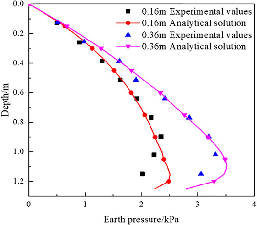
FIGURE 8. Comparison of lateral earth pressure.

Take and Valsangkar. (2001) performed a centrifuge model test in which both the retaining wall back and rock surface were in the vertical direction. The maximum and minimum dry densities of non-cohesive fillers were 1.62 g/cm³ and 1.34 g/cm³, respectively. Their relative compactness was 79%. The internal friction angles corresponding to the peak value and the critical state were 36° and 29°, respectively. In the test, the peak value of the wall–soil friction angle was 25°, and the critical value was 23°. The acceleration adopted in the test was 35.7 g (where g is the gravity acceleration). As a result, the retaining wall model with a height of 140 mm in the test after centrifugal amplification was equivalent to the retaining wall with a height of 5 m in reality. The limited filling widths are L = 15 and 38 mm, which are equivalent to the filling widths b = 0.54 and 1.36 m. In this study, the calculation and model tests are compared.

It can be seen from Figure 9 that the theoretical value of finite soil pressure strength calculated in this study is close to the experimental value. The range of the maximum value is also the same. The results are similar in the depth range of 2∼4.5 m, but the experimental value in the depth range of 0.5∼1.5 m has a large discreteness, which is different from the theoretical value. More finite soil centrifuge tests are needed to verify.

FIGURE 9

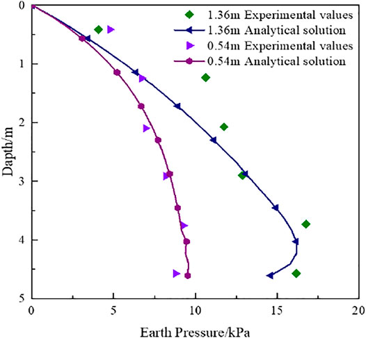
FIGURE 9. Comparison of lateral earth pressure.

Critical Width of Finite Soil

Determination of the Critical Width

Geotechnical engineering is concerned with determining the critical width of finite soil. The width calculated by the Coulomb earth pressure theory is commonly used as the critical value by most researchers. However, the critical width of the soil is not accurate because the Coulomb earth pressure assumes that the sliding surface behind the wall is straight.

Based on this, after deriving ${\theta }_{\text{c}}$ by the aforementioned method, the slip crack surface width X₀ can be deduced as:

$X_{\text{0}}=R_1({\theta }_c-\sin {\theta }_c),(33)$

This study selects the retaining wall height of 10 m, the filling weight of 14.6 kN/m³, and the filling surface without load as examples to investigate the influence of various parameters on the critical width of finite soil.

Effects of the Internal Friction Angle

The wall–soil friction angle is taken as a fixed value ${\delta }_1=20°$. The internal friction angle is varied for analysis. The critical slip surface of the finite soil and semi-infinite soil is shown in Figure 10. The corresponding critical widths of the finite soil are 5.41, 4.63, 4.08, 3.56, and 3.11 m. At this time, the critical widths calculated according to the Coulomb earth pressure theory are 6.75, 5.92, 5.18, 4.52, and 3.92 m. It can be seen that when the internal friction angle increases, the critical width of the finite soil decreases gradually. The change rate also decreases gradually. The critical width value obtained by this method is obviously smaller than the calculated value of Coulomb earth pressure.

FIGURE 10

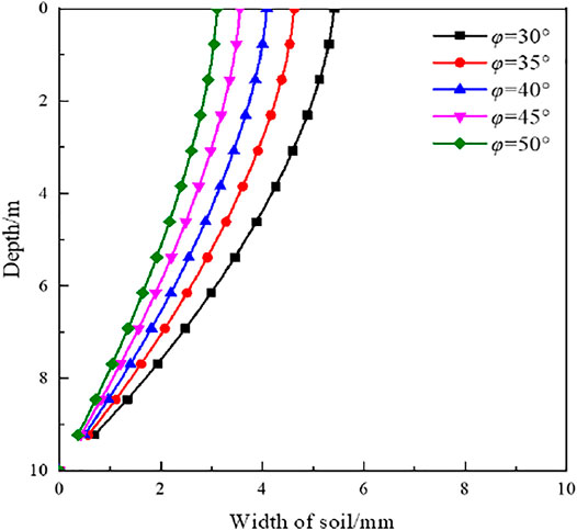
FIGURE 10. Influence of the internal friction angle on the slip surface.

Effects of the Wall–Soil Friction Angle

The internal friction angle is taken as $\phi =40°$ and the wall–soil friction angle is taken as ${\delta }_1=10°,20°,30°,40°$ for analysis. The critical slip surface of the finite soil and semi-infinite soil is shown in Figure 11. The corresponding critical widths of the finite soil are 3.89, 4.08, 4.42, and 5.05 m, respectively. At this time, the critical widths calculated according to the Coulomb soil pressure theory are 4.94, 5.18, 5.42, and 5.67 m. The results show that when the wall–soil friction angle increases, the critical width of the finite soil gradually increases, and the change rate gradually increases. The critical width of finite soil is smaller than the Coulomb theoretical value under different wall–soil friction angles.

FIGURE 11

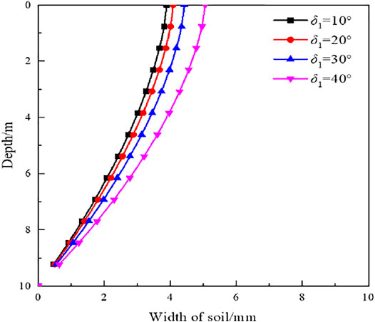
FIGURE 11. Influence of the friction angle between the wall and soil on the slip surface.

Conclusion

This study derives the soil pressure distribution of non-cohesive soil with finite width behind the retaining wall based on the assumption that the soil behind the retaining wall has a cycloidal slip surface. The following conclusions can be drawn:

1) For the case of finite non-cohesive soil behind the retaining wall, a method for calculating the active earth pressure of soil with finite width is proposed based on the failure mode of the cycloidal line sliding surface passing through the wall toe caused by the translation of the retaining wall. This method considers the principal stress deflection induced by the friction between the wall and the soil and assumes that the trajectory of the minor principal stress is a circular arc.

2) According to the theoretical equations, the distribution law of active earth pressure of finite soil is obtained. When the retaining wall moves horizontally, the soil pressure of the finite soil behind the wall presents a nonlinear drum distribution along the height direction of the retaining wall. The maximum soil pressure distribution is close to the bottom of the wall.

3) The calculation method of the critical width of finite soil is proposed. The critical width of a retaining wall decreases as the internal friction angle of the soil increases during the translation process and increases with the increase of wall–soil friction angle. The critical width of finite soil obtained by this method is smaller than the critical width value calculated by the Coulomb earth pressure theory.

4) This study analyzes the earth pressure of the non-cohesive soil and rigid retaining wall. In practical engineering, there may be cohesive soil or multi-layer soil behind the wall. Meanwhile, there are also many flexible retaining walls. Subsequently, the earth pressure distribution of finite soil will be further investigated in the case of flexible retaining wall structure and clay filling.

Data Availability Statement

The original contributions presented in the study are included in the article/Supplementary Material, further inquiries can be directed to the corresponding authors.

Author Contributions

KH: conceptualization, investigation, and writing—original draft. RL: investigation and methodology. YS: data curation and methodology. LL: writing—review and editing. YX: data curation and methodology. XP: provided data support.

Funding

The work presented in this article was supported by the National Natural Science Foundation of China (Grant No. 52078060), National Science Foundation of Hunan Province (Grant No. 2020JJ4606), International Cooperation and Development Project of Double-First-Class Scientific Research in Changsha University of Science and Technology (Grant No. 2018IC19), and Innovative Program of Key Disciplines with Advantages and Characteristics of Civil Engineering of Changsha University of Science and Technology (Grant No. 18ZDXK05).

Conflict of Interest

YS was employed by the company Shanghai Harbour Foundations Construction Group Ltd. XP was employed by the company The First Engineering Co., Ltd., China Railway No. 5 Bureau Group.

The remaining authors declare that the research was conducted in the absence of any commercial or financial relationships that could be construed as a potential conflict of interest.

Publisher’s Note

All claims expressed in this article are solely those of the authors and do not necessarily represent those of their affiliated organizations, or those of the publisher, the editors, and the reviewers. Any product that may be evaluated in this article, or claim that may be made by its manufacturer, is not guaranteed or endorsed by the publisher.

References

Cao, Z.-M. (1995). Active Earth Pressure Analysis on Retaining wall with Sliding Surface of Filling Curve. China J. Highw. Transport 8 (S1), 7–14. doi:10.19721/j.cnki.1001-7372.1995.s1.002

CrossRef Full Text | Google Scholar

Greco, V. (2013). Active Thrust on Retaining walls of Narrow Backfill Width. Comput. Geotechnics 50, 66–78. doi:10.1016/j.compgeo.2012.12.007

CrossRef Full Text | Google Scholar

Handy, R. L. (1985). The Arch in Soil Arching. J. Geotechnical Eng. 111 (3), 302–318. doi:10.1061/(asce)0733-9410(1985)111:3(302)

CrossRef Full Text | Google Scholar

He, Z.-M., Liu, Z.-F., Liu, X.-H., and Bian, H.-b. (2020). Improved Method for Determining Active Earth Pressure Considering Arching Effect and Actual Slip Surface. J. Cent. South. Univ. 27 (7), 2032–2042. doi:10.1007/s11771-020-4428-5

CrossRef Full Text | Google Scholar

Hu, W.-D., Cao, W.-G., and Zeng, L.-X. (2018). Upper Bound Solution of Earth Pressure for Limited Soils Adjacent to Existing Buildings Considering Friction Energy Consumption. Hydrogeology Eng. Geology. 45 (05), 73–79+85. doi:10.16030/j.cnki.issn.1000-3665.2018.05.10

CrossRef Full Text | Google Scholar

Huang, K., Sun, Y.-W., Sun, Y., He, J., Huang, X., Jiang, M., et al. (2021b). Comparative Study on Grouting protection Schemes for Shield Tunneling to Adjacent Viaduct Piles. Adv. Mater. Sci. Eng. 2021, 1–19. doi:10.1155/2021/5546970

CrossRef Full Text | Google Scholar

Huang, K., Sun, Y.-W., Yang, J.-S., Li, Y.-J., Jiang, M., and Huang, X.-Q. (2022). Three-dimensional Displacement Characteristics of Adjacent Pile Induced by Shield Tunneling under the Influence of Multiple Factors. J. Cent. South Univ. 29, 5003. doi:10.1007/s11771-022-5003-z

CrossRef Full Text | Google Scholar

Huang, K., Sun, Y.-W., Zhou, D.-Q., Li, Y.-J., Jiang, M., and Huang, X.-Q. (2021a). Influence of Water-Rich Tunnel by Shield Tunneling on Existing Bridge Pile Foundation in Layered Soils. J. Cent. South. Univ. 28 (8), 2574–2588. doi:10.1007/s11771-021-4787-6

CrossRef Full Text | Google Scholar

Khosravi, M. H., Pipatpongsa, T., and Takemura, J. (2013). Experimental Analysis of Earth Pressure against Rigid Retaining walls under Translation Mode. Géotechnique 63 (12), 1020–1028. doi:10.1680/geot.12.P.021

CrossRef Full Text | Google Scholar

Liu, C., Fang, D., and Zhao, L. (2021). Reflection on Earthquake Damage of Buildings in 2015 Nepal Earthquake and Seismic Measures for post-earthquake Reconstruction. Structures 30, 647–658. doi:10.1016/j.istruc.2020.12.089

CrossRef Full Text | Google Scholar

Liu, Z.-Y. (2018). Active Earth Pressure Calculation of Rigid Retaining walls with Limited Granular Backfill Space. China J. Highw. Transport 31 (2), 154–164. doi:10.19721/j.cnki.1001-7372.2018.02.016

CrossRef Full Text | Google Scholar

Paik, K. H., and Salgado, R. (2003). Estimation of Active Earth Pressure against Rigid Retaining walls Considering Arching Effects. Géotechnique 53 (7), 643–653. doi:10.1680/geot.2003.53.7.643

CrossRef Full Text | Google Scholar

Take, W. A., and Valsangkar, A. J. (2001). Earth Pressures on Unyielding Retaining walls of Narrow Backfill Width. Can. Geotech. J. 38 (6), 1220–1230. doi:10.1139/t01-063

CrossRef Full Text | Google Scholar

Wang, K.-H., Ma, S.-J., and Wu, W.-B. (2011). Active Earth Pressure of Cohesive Soil Backfill on Retaining wall with Curved Sliding Surface. J. Southwest Jiaotong Univ. 46 (5), 732–738. doi:10.3969/j.issn.0258-2774.2011.05.004

CrossRef Full Text | Google Scholar

Wang, Y.-C., Yan, E.-C., and Lu, W.-B. (2016). Analytical Solution of Active Earth Pressure for Limited Cohesionless Soils. Rock Soil Mech. 37 (9), 2513–2520. doi:10.16285/j.rsm.2016.09.011

CrossRef Full Text | Google Scholar

Wu, C.-F., Zhang, Z.-J., and Liu, S.-H. (2014). Calculation Method for Lateral Earth Pressure on Parallel Retaining walls with Clayey Backfill Considering Soil Arching Effect. China J. Highw. Transport 27 (04), 31–37. doi:10.19721/j.cnki.1001-7372.2014.04.005

CrossRef Full Text | Google Scholar

Xu, C., Chen, Q., Luo, W., and Liang, L. (2019). Analytical Solution for Estimating the Stress State in Backfill Considering Patterns of Stress Distribution. Int. J. Geomech. 19 (1), 04018189. doi:10.1061/(ASCE)GM.1943-5622.0001332

CrossRef Full Text | Google Scholar

Xu, R.-Q., Xu, Y.-B., and Cheng, K. (2020). Method to Calculate Active Earth Pressure Considering Soil Arching Effect under Non-limit State of clay. Chin. J. Geotechnical Eng. 42 (02), 362–371. doi:10.11779/CJGE202002018

CrossRef Full Text | Google Scholar

Yang, M.-H., Dai, X.-B., and Zhao, M.-H. (2016). Experimental Study on Active Earth Pressure of Cohesionless Soil with Limited Width behind Retaining wall. Chin. J. Geotechnical Eng. 38 (1), 723–728. doi:10.11779/CJGE201601014

CrossRef Full Text | Google Scholar

Yang, M.-H., Wu, Z.-Y., and Zhao, M.-H. (2020). Soil Arch Effect Analysis and Earth Pressure Calculating Method for Finite Width Soil behind Retaining wall. J. Hunan Univ. (Natural Sciences) 47 (03), 19–27. doi:10.16339/j.cnki.hdxbzkb.2020.03.003

CrossRef Full Text | Google Scholar

Yang, G, G., Wang, Y.-Y., and Liu, Y.-C. (2017). Analysis of Active Earth Pressure on Retaining walls Based on Curved Sliding Surface. Rock Soil Mech. 38 (8), 2182–2188. doi:10.16285/j.rsm.2017.08.004

CrossRef Full Text | Google Scholar

Yang, M. H, M.-H., Dai, X.-B., and Zhao, M.-H. (2017). Calculation of Active Earth Pressure for Limited Soils with Curved Sliding Surface. Rock Soil Mech. 38 (7), 2029–2035. doi:10.16285/j.rsm.2017.07.024

CrossRef Full Text | Google Scholar

Zhao, Q., and Zhu, J.-M. (2014). Research on Active Earth Pressure behind Retaining wall Adjacent to Existing Basements Exterior wall Considering Soil Arching Effects. Rock Soil Mech. 35 (3), 723–728. doi:10.16285/j.rsm.2014.03.007

CrossRef Full Text | Google Scholar

Zhu, J.-M., and Zhao, Q. (2014). Unified Solution to Active Earth Pressure and Passive Earth Pressure on Retaining wall Considering Soil Arching Effects. Rock Soil Mech. 35 (9), 2501–2505. doi:10.16285/j.rsm.2014.09.006

CrossRef Full Text | Google Scholar