
94% of researchers rate our articles as excellent or good
Learn more about the work of our research integrity team to safeguard the quality of each article we publish.
Find out more
ORIGINAL RESEARCH article
Front. Earth Sci., 03 May 2022
Sec. Marine Geoscience
Volume 10 - 2022 | https://doi.org/10.3389/feart.2022.882617
This article is part of the Research TopicSedimentation on the Continental Margins: From Modern Processes to Deep-Time RecordsView all 28 articles
 Meinan Shi1,2,3
 Huaichun Wu1,2,3*
 Eric C. Ferré4
 Sara Satolli5
 Qiang Fang1,2,3
 Yunfeng Nie1,2,3Yuhe Qin1,2,3Shihong Zhang1
 Tianshui Yang1Haiyan Li1
Site U1501 of International Ocean Discovery Program (IODP) Expedition 368 locates on a broad regional basement high in the northern margin of the South China Sea (SCS). This study refines the chronostratigraphy of the upper 160 m sedimentary succession from Hole U1501C using paleomagnetic measurements and cyclostratigraphic analysis on the Natural Gamma Radiation (NGR) data. Rock magnetic analysis displays that the magnetic signal of the sediments is mainly carried by single-domain (SD) and multi-domain (MD) magnetite. A total of 12 geomagnetic reversals are identified and correlated to the geomagnetic polarity time scale (GPTS) in Geologic Time Scale 2020 (GTS 2020), combining biostratigraphic data and planktonic foraminiferal oxygen records. The Milankovitch cycles of 405-kyr long orbital eccentricity, ∼100-kyr short orbital eccentricity, and obliquity cycles are identified in the NGR profile. A 15.54 Myr astronomical time scale is constructed by tuning the short eccentricity cycles filtered from the NGR profiles to the La2010 astronomical solution with the constraints of the magnetostratigraphic results, biostratigraphic age datum and planktonic foraminiferal oxygen records. This new high-resolution age model provides a new temporal constraint on the tectonic and paleoenvironmental evolution in the South China Sea.
The South China Sea (SCS), the largest marginal sea in the low latitude West Pacific region, has a series of advantages in deep-sea research, and becomes into the international deep-sea frontiers to explore important scientific issues such as the opening of the marine basin and Cenozoic paleoclimate evolution (especially in the aspects of climate periodic evolution), the low-latitude forcing in carbon cycling, East Asian monsoon, etc. (Clift et al., 2014; Wang et al., 2014; Wang and Jian, 2019). IODP Site U1501 locates on a broad regional basement high in the northern margin of the SCS (Figure 1). It was drilled during IODP Expedition 368, which aimed to test the scientific hypotheses of the breakup of the northern SCS margin.
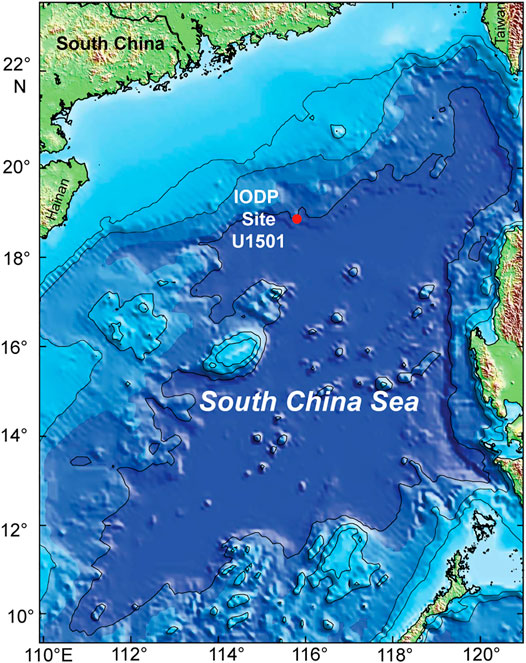
FIGURE 1. Location of the IODP Site U1501 in the SCS (modified from Sun et al., 2016).
Site U1501 recovers the sedimentary succession evolving from land to deep sea (Larsen et al., 2018) and can greatly help understanding the sedimentary processes associated with the breakup of the SCS continental margin and tectonic events. The water depth (2,850 m) at Site U1501 makes it one of the few sites above the modern carbonate compensation depth (CCD) of the SCS. Its deposits, rich in calcareous microfossils, are the focus of scientific objectives related to 1) reconstructing the history of the East Asian monsoon evolution and of deep water exchanges between the SCS and the Pacific Ocean and 2) exploring the sedimentary responses to the Cenozoic regional tectonic and environmental development of the Southeast Asia margin (Larsen et al., 2018). In order to address the above scientific objectives, accurate dating and scaling of key geologic boundaries is required, which provides estimates of durations of major geological events and the correlation of stratigraphic records from other sites.
Establishing the magnetostratigraphic time framework depends on extracting native and reliable geomagnetic reversal or drift signals recorded on primary magnetic minerals in the marine environment. However, the reliability of onboard paleomagnetic results from Hole U1501C has been hampered by the presence of greigite, maghemite, or hematite in the upper 83 m (Larsen et al., 2018). Onboard biostratigraphy (Figure 2H; Larsen et al., 2018) was mainly based on the analysis of core catcher samples, which may encase the ex-situ material and cause some uncertainties. Post-expedition calcareous nannofossil assemblages study based on post-expedition samples collected from the working-half sections provided an updated biostratigraphic framework between 5 and 15 Ma, showing ages significantly older than the shipboard ones (Wang and Jiang, 2020). Furthermore, the post-expedition planktonic foraminiferal oxygen records of the upper 46 m of Site U1501 were constrained by shipboard age datum (Zhang et al., 2020; Figure 2H). Therefore, the preliminary chronostratigraphy results from Site U1501 (Larsen et al., 2018) need to be improved to provide a reliable age model.
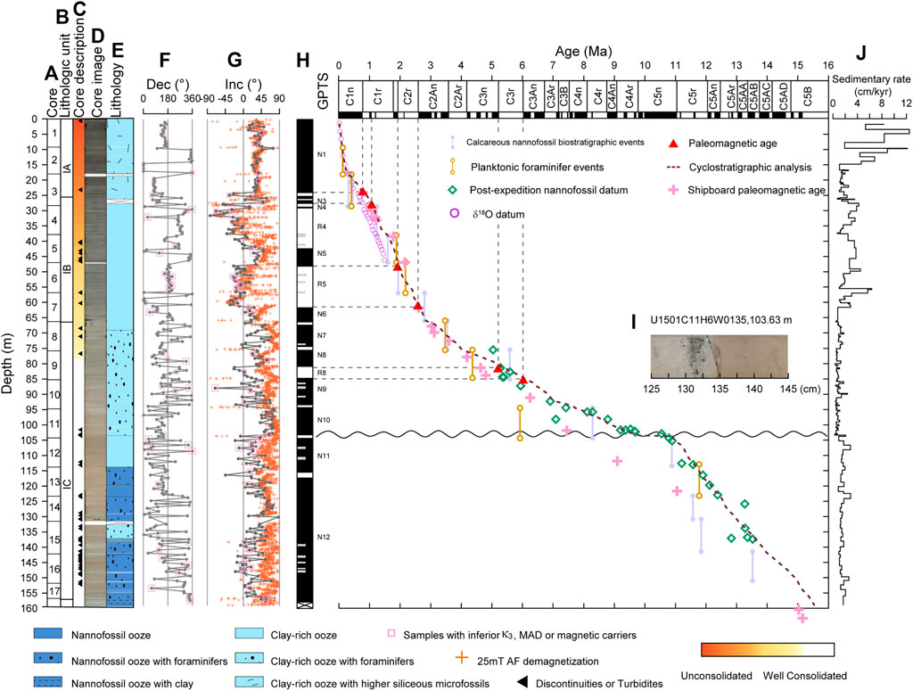
FIGURE 2. Magnetostratigraphic interpretation of the IODP Hole U1501C, Expedition 368. (A) Core number. (B) Lithologic unit. (C) Core description about consolidation, continuities condition and turbidites. Leftward-pointing triangles represent the presence of discontinuities or turbidites. (D) Core image. (E) Lithology. (F–G) Declination and inclination of the paleomagnetic data. Pink boxes represent the samples with unaccepted κ3, MAD and magnetic carriers; orange crosses represent shipboard 25 mT alternating field demagnetization results. (H) The sequence of paleomagnetic polarity interpretations correlated to the GPTS in GTS 2020 (Ogg, 2020). Black, white, and half gray intervals represent normal, reversal, and uncertainty polarities, respectively. Red triangles represent the magnetostratigraphic age model yielded in this study. Pink crosses represent shipboard paleomagnetic age (Larsen et al., 2018), powder blue and light orange symbols represent calcareous nannofossil biostratigraphic events and planktonic foraminifer events (Larsen et al., 2018), green diamonds represent post-expedition nannofossil datum (Wang and Jiang, 2020). Purple circles represent the δ18O isotopic records (Zhang et al., 2020). Brown curves represent the astrochronologic results. (I) The core photo showing the sedimentary hiatus at ∼103.63 m is shown. (J) The variations of sediment accumulation rates are based on magneto-astrochronologic results.
Here, we enhance the chronostratigraphy of the upper 160 m sedimentary succession from Site U1501 combining systematic paleomagnetic measurements and cyclostratigraphic analysis on NGR with shipboard and post-expedition biostratigraphy. The reliability of the magnetostratigraphy is reached by decreasing the sampling interval and analyzing the magnetic mineralogy of sediments and the mechanism of remanence magnetization. The acquisition of the high-resolution integrated magneto-cyclostratigraphic time scale of sediments in the northern SCS will play a vital role in achieving the scientific objectives of the IODP Expedition 368 and promote the understanding of the tectonic and environmental evolution of the SCS.
A 160 m thick sedimentary succession was recovered from lithostratigraphic Unit I of Hole U1501C (18°53.0910’N, 115°45.9485’E; 2,846 m below seafloor) cored with the advance piston corer (APC) system. The dominant lithologies are nannofossil ooze, with minor nannofossil-rich clay, rare foraminiferal sand, and sandy silt. 312 cubic samples were collected using standard 2 × 2 × 2 cm plastic boxes with 0.5 m sampling resolution from the central part of working-halves to reduce the effect of drilling disturbance. NGR data (∼10-cm spacing) was used as a paleoclimatic indicator related to lithology. High NGR values are associated with clay-rich sediments and lower NGR values with coarse-grained or carbonate-rich sediments (e.g., Zhang et al., 2019).
All the rock magnetic and paleomagnetic measurements were performed at the Paleomagnetism and Environmental Magnetism Laboratory at China University of Geosciences, Beijing, and the Institute of Geophysics, China Earthquake Administration, respectively.
Rock magnetic experiments were conducted to understand the nature and origin of the remanence carriers and to establish the appropriate demagnetization procedures. Low-frequency magnetic susceptibility (χ, mass-specific) and anisotropy of magnetic susceptibility (AMS) were measured using the MFK1-FA Kappabridge. Data generated from the AMS measurements include the maximum, intermediate and minimum susceptibility axes (κ1> κ2 > κ3) of the magnetic susceptibility ellipsoids, the lineation parameter L (κ1/κ2) and the flattening parameter F (κ2/κ2), the anisotropy degree P (κ1/κ3) and the shape parameter T [(2κ2-κ1-κ3)/(κ1-κ3)]. Temperature dependence of low-field magnetic susceptibilities (χ-T) was measured in an argon atmosphere to avoid oxidation of the magnetic minerals, using a KLY-4S Kappabridge magnetic susceptibility meter with a temperature apparatus (CS-3). Saturation isothermal remanent magnetization (SIRM) acquired in a field of 2 T was applied using an ASC IM-10–30 impulse magnetizer. Hysteresis measurements, including first-order reversal curve (FORC), isothermal remanent magnetization (IRM) acquisition curves, and direct field demagnetization curves, were performed using a MicroMag Model 3,900 Vibrating Sample Magnetometer. FORC diagrams processed by Forcinel v3.06 (Harrison and Feinberg, 2008) are described by a hysteron with a specified coercivity Bc, and horizontal offset Bu. The unmixing of IRM curve (Kruiver et al., 2001) is used for evaluating the carriers of magnetic remanence. Each magnetic component is characterized by its SIRM, mean coercivity B1/2, and dispersion parameter (DP). Remanent coercive force (Bcr) was determined from direct field demagnetization curves.
A total of 290 discrete samples were subjected to progressive alternating field (AF) demagnetization at peak fields up to 120 mT (16 steps) using a D-2000 AF demagnetizer. 22 samples were analyzed with thermal demagnetization (TD) up to 600°C (27 steps) using an ASC TD-48 furnace with an internal residual field of less than 10 nT. Remanent magnetization measurements were carried out with a 2G-755-4K cryogenic magnetometer located in a shielded room.
NGR data have been widely used to analyze paleoclimatic variations and to reveal the sedimentary cycles in marine and nonmarine sediment successions (e.g., Wu et al., 2013; Li et al., 2017; Zhang et al., 2019). The raw NGR profile from Site U1501 (Supplementary Figure S1) was interpolated to a uniform spacing of 10 cm, then long periods (>6 m) were removed using moving smoothing in Matlab.
The spectral analysis was performed using the multitaper method (MTM; Thomson, 1982) with a classical red noise modeling in “Acycle” software (Li et al., 2019). Evolutionary Fast Fourier transform analysis (FFT; Kodama and Hinnov, 2015) was conducted to identify changes in spatial and temporal cycle frequencies. The interpreted orbital cycles were extracted from data series using Taner bandpass filters and were tuned to the La2010 astronomical solution (Laskar et al., 2011). The tuning process was performed on the freeware Analyseries 2.0.8 (Paillard et al., 1996).
Magnetic susceptibility drops around 580°C in most heating curves (Figures 3A–D), suggesting magnetite is the main magnetic carrier (Dunlop and Özdemir, 1997). Some samples display a pronounced increase of magnetic susceptibility at 320°C (Figure 3B) and/or a slight decrease at 600–700°C (Figure 3A), suggesting the presence of iron sulfide and/or hematite. FORC diagrams, a powerful tool to visualize the domain state of magnetic minerals, mainly show the MD + SD behavior (Figures 3E,G,H). Few samples have contours centering a single-domain peak with coercivity (Bc) around 65 mT (Figure 3F), indicating the contribution of greigite. The unmixing of IRM curve (Kruiver et al., 2001) is used for evaluating the carriers of magnetic remanence. Each magnetic component is characterized by its SIRM, mean coercivity B1/2, and dispersion parameter (DP). Four component types were identified (Figures 3 I–L) including coarse magnetite grain (<40 mT mean coercivity), fine magnetite grain (∼50 mT mean coercivity with narrow coercivity distribution), greigite (∼60–80 mT with narrow coercivity distribution), and hematite (B1/2 > 100 mT). Biplot of the SIRM/χ versus Bcr, used for distinguishing the type of the magnetic minerals (Peters and Thompson, 1998; Figure 4), indicates that the predominant carrier of remanent magnetization is magnetite. The greigite has limited influence on the paleomagnetic study.
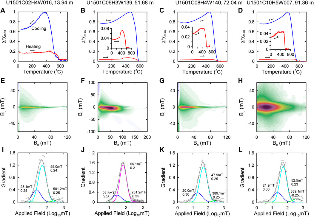
FIGURE 3. Rock magnetic results of representative samples from Site U1501. (A–D) High-temperature magnetic susceptibility (χ-T) curves. Red and blue lines represent heating and cooling curves, respectively. The susceptibility curves are normalized by the susceptibility maximum (χmax). (E–H) First-order reversal curve (FORC) diagrams (smooth factor = 3). (I–L) Isothermal remanent magnetization (IRM) component analysis. Grey squares represent data points that define the gradient of IRM acquisition curves. Grey lines are the fitted total spectra. Blue, cyan, pink, and green lines represent the coarse grain size magnetite, fine grain size magnetite, greigite and hematite, respectively. The values for B1/2 and DP of each component are listed.
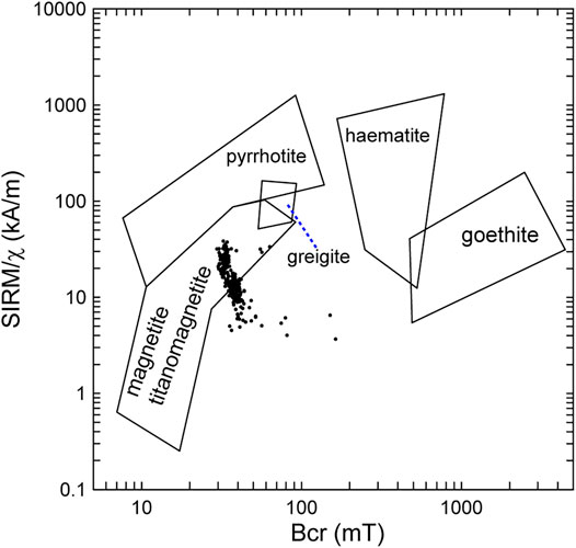
FIGURE 4. Biplot of SIRM/χ and Bcr of samples from Site U1501.
The AMS shows that the minimum susceptibility axes (κ3) of most samples are perpendicular to the bedding plane, while the maximum (κ1) and medium (κ2) susceptibility axes lie in the bedding plane (Figure 5A). Plots of shape parameter (T) versus anisotropy degree (P), and lineation (L) versus foliation (F) show a dominance of the oblate form (Figures 5B,C). These results indicate that most samples have undisturbed sedimentary fabrics.
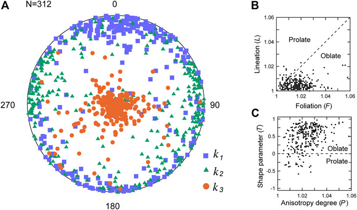
FIGURE 5. Anisotropy of magnetic susceptibility (AMS) results of Site U1501. (A) Lower hemisphere equal-area projection of AMS data. Blue squares, green triangles, and brown circles represent directions of maximum (κ1), intermediate (κ2), and minimum (κ3) susceptibility axes, respectively. (B) plot of lineation (L) versus foliation (F), and (C) plot of shape parameter (T) versus anisotropy degree (P).
Magnetic components were calculated by principal component analysis (PCA) (Kirschvink, 1980) using the software PaleoMag (Jones, 2002). A component with the steep positive inclination can be removed before 30 mT or 250°C (Figure 6), which is most likely an overprint induced by the coring process that was identified in many paleomagnetic studies on the ODP/IODP cores (Acton et al., 2002; Tauxe et al., 2012; Zhao et al., 2013). The characteristic remanent magnetization (ChRM) was identified through the stepwise AF demagnetization with a maximum field of 80–120 mT or thermal demagnetization (TD) up to 600°C.
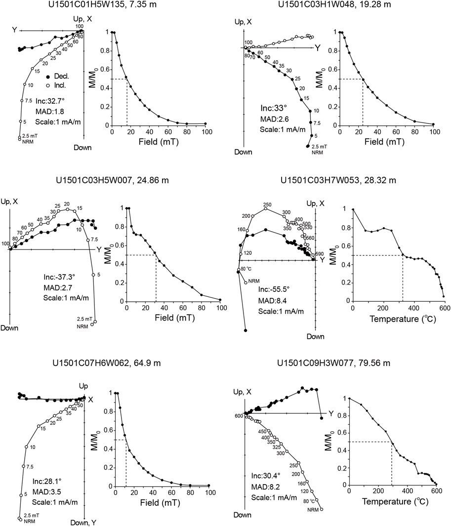
FIGURE 6. Typical demagnetization orthogonal projections (left, Zijderveld, 1967) and normalized magnetization curves as a function of alternating field (thermal) demagnetization (right). The solid and open circles in demagnetization orthogonal projections represent the projection of the magnetization vector endpoint on the horizontal and vertical planes.
For samples from IODP Site U1501, polarity ambiguity arises because the samples are azimuthally unoriented and the expected inclination ∼25.5° is relatively shallow. We applied the following methods to establish the magnetozones: (a) positive/negative inclination (±37.3 ± 6.6°) corresponding to a paleolatitude of ±20.8 ± 3.3°N is interpreted as normal/reversed polarity, respectively. (b) polarity reversal is identified by near 180° shift in declinations on long coherent core sections. In order to obtain reliable magnetic polarity zones, the samples with the following scenarios are discarded from the magnetostratigraphic interpretation: (a) greigite as the dominated magnetic carrier, (b) inclination of κ3 axes of the AMS less than 60°, and (c) maximum angular deviation (MAD) larger than 15°. A succession of 12 normal and 11 reversed events are recognized, while some suspected reversed events with only one or two samples are also shown (Figure 2H).
The sedimentary succession of Hole 1501C is characterized by a hiatus at 103.63 m (section U1501C11H6W, 135 cm), marked by significant discontinuity and downhole color change based on the core section image (Figure 2I) and spanning approximately 10.5–9.0 Ma (Wang and Jiang, 2020). Assuming there are no other significant hiatuses, an initial magnetostratigraphic scale (Table 1; Figure 2) was constructed by correlating observed polarity sequences with a reference GPTS in GTS 2020 (Ogg, 2020), constrained by shipboard and post-expedition biostratigraphy (Larsen et al., 2018; Wang and Jiang, 2020) and δ18O isotopic record (Zhang et al., 2020).
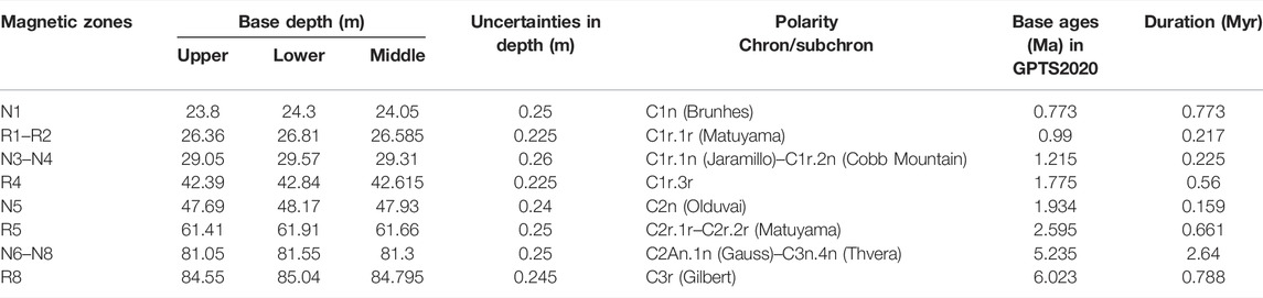
TABLE 1. Correlation of the magnetostratigraphy of IODP Hole U1501C (0–160 m) to the GPTS in GTS 2020 (Ogg, 2020).
The base of magnetozone N1 correlates with the base of Chron C1n (Brunhes) (Figure 2H), according to shipboard paleomagnetic results (Larsen et al., 2018). The top of magnetozone N5 has a date of 1.36–1.88 Ma based on the shipboard biostratigraphy (last appearance of Calcidiscus macintyrei (1.6 Ma) and Globigerinoides fistulosus (1.88 Ma) at 38.08–46.95 m; Larsen et al., 2018) and δ18O isotopic record (42 m, 1.36 Ma; Zhang et al., 2020), thus correlates with the top of C2n (Olduvai). Uncertainty polarities below the N5 make us tend to connect the base of N5 and C2n (Olduvai), which is slightly younger than the shipboard magnetic age located at the base of C2r.1n (Feni). According to shipboard paleomagnetic results, the base of polarity zone R5 correlates with the base of C2r.2r (Matuyama). A series of biological events including the last appearance of Triquetrorhabdulus/Orthorhabdus rugosus (81.74 m, 5.28 Ma), Discoaster quinqueramus (83.09 m, 5.59 Ma) and Nicklithus amplificus (87.65 m, 5.94 Ma), and the first appearance of Ceratolithus acutus (84.77 m, 5.35 Ma) and Ceratolithus atlanticus (84.77 m, 5.39 Ma), display the age of sediment from 82–88 m is 5.28–5.94 Ma (Wang and Jiang, 2020), supporting the correlation of magnetozones N6–N8 to Chrons C2An.1n (Gauss)–C3n.2n (Nunivak). Finally, polarity zone R8 correlates with Chron C3r (Gilbert). Below 85.04 m, dominant normal polarities hamper the determination of magnetic polarities.
The magnetostratigraphic and biostratigraphic results (Figure 2H) constrained a timescale for Site U1501. A higher resolution age model is constructed using astrochronologic analysis on three separate intervals: 0–66 m, 66–103.6 m, and 103.6–160 m. In fact, the subunit IB/IC boundary at 66.17–66.3 m is marked by an abrupt change in NGR (Supplementary Figure S1) and lithology (Figures 2D,E; Larsen et al., 2018). Sediment in subunit IC displays a lower sedimentary rate than subunit IB based on shipboard age datum (Figure 2H). In addition, as mentioned above, there is a hiatus at 103.63 m.
The NGR series in the 0–66 m interval has been converted to the time domain (Figure 7A) based on the initial paleomagnetic results including the base of N1 (Chron C1n) and N5 (Chron C2n) and the top of N6 (the top of Chron C2An.1n) and oxygen isotopic records (Figure 2H). Zhang et al. (2020) obtained the planktonic foraminiferal oxygen records (Globigerinoides ruber) of the upper 46 m of Site U1501 (Figure 8A). However, the establishment of their age model was based on the shipboard biostratigraphy model, which has a discrepancy with paleomagnetic results here. Therefore, this study adopts the age-depth points until 18 m, where the feature of the δ18O curve is largely compatible with the LR04 stack (Lisiecki and Raymo, 2005). Then age points including MIS 22, 36, 37, and 54 were determined based on oxygen isotope features around the boundary of polarity zones of C1n, C1r.2n, and C2n (Figure 8A).
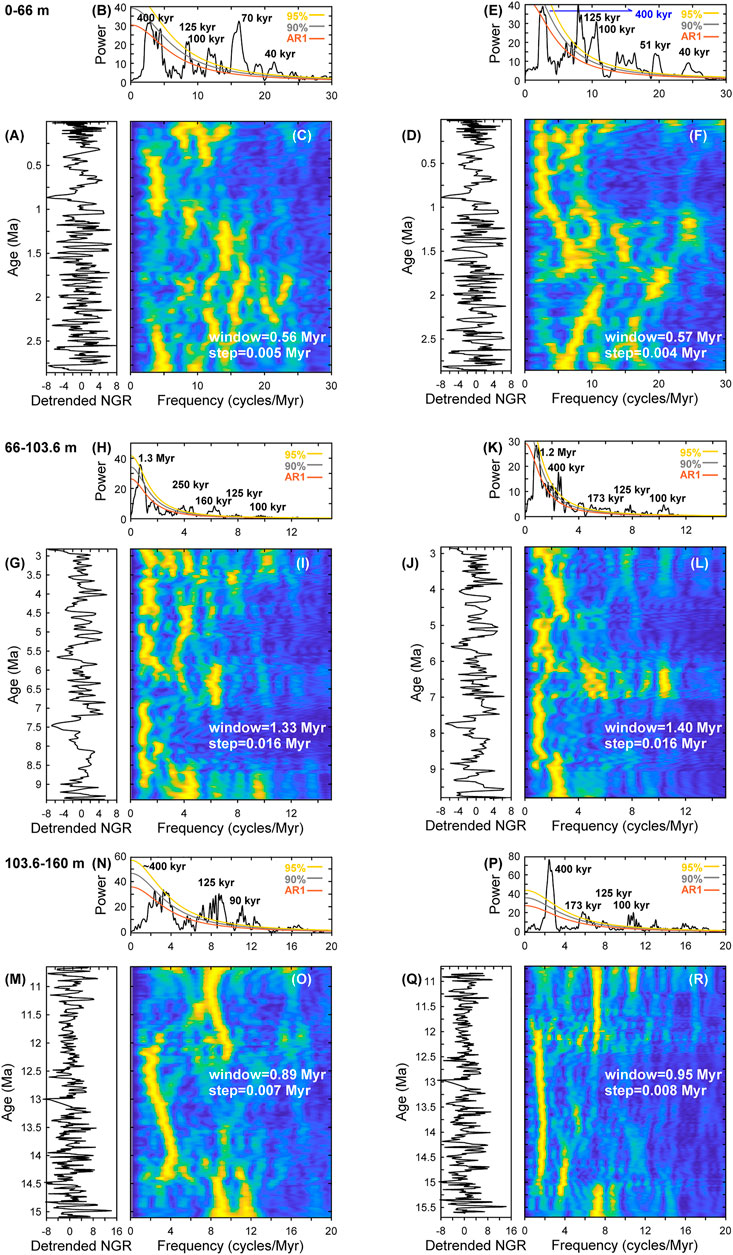
FIGURE 7. The detrended NGR data in time domain constraint by initial age anchors of magnetostratigraphy, biostratigraphy and planktonic foraminiferal oxygen records (A,G,M) and its 2π MTM spectral analysis (B,H,N) and evolutionary power spectrum (C,I,O). The 100 kyr tuned detrended NGR series (D,J,Q) and their 2π MTM power spectrum (E,K,P) and evolutionary power spectrum (F,L,R).
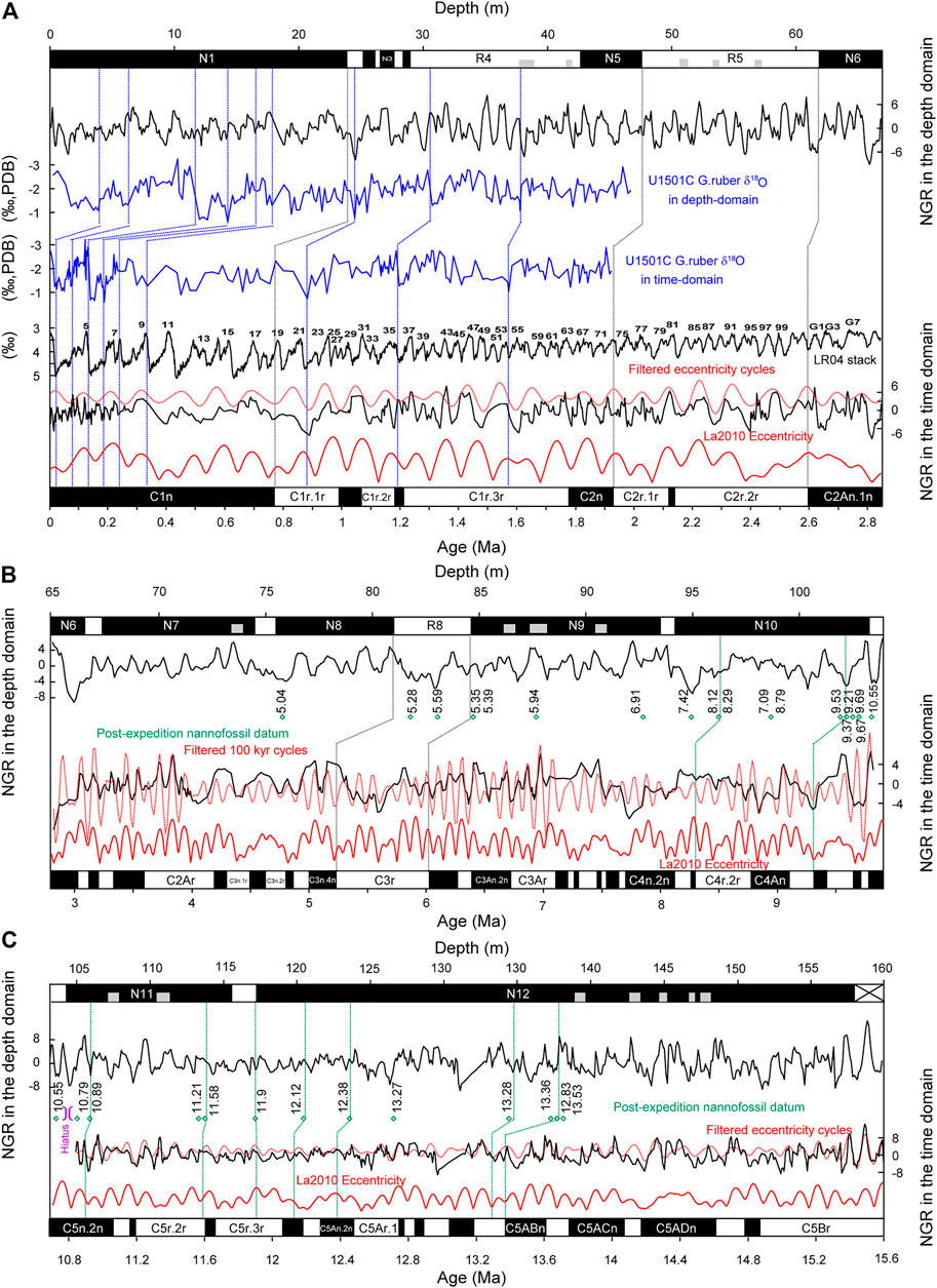
FIGURE 8. (A) Correlations of NGR in the depth interval of 0–65 m to La2010 orbital eccentricity curves (Laskar et al., 2011). From top to bottom: interpretative paleomagnetic polarity zones; the detrended NGR data in the depth interval of 0–65 m; δ18O records of the U1501 (Zhang et al., 2020) in depth-domain and time domain; the LR04 stack (Lisiecki and Raymo, 2005). Tuned NGR data in time-domain and its short eccentricity filters with passbands of 9 ± 2 cycles/Ma. La2010 orbital eccentricity curves (Laskar et al., 2011); GPTS in GTS 2020 (Ogg, 2020). Correlations of NGR in the depth interval of 66–103.6 m (B) and 103.6–160 m (C) to La2010 orbital eccentricity curves (Laskar et al., 2011). From top to bottom: interpretative paleomagnetic polarity zones; the detrended NGR data in the depth domain; post-expedition nannofossil datum (green diamonds; Wang and Jiang, 2020); the tuned NGR data in time-domain and its short eccentricity filters with passbands of 9 ± 2 cycles/Ma; La2010 orbital eccentricity curves (Laskar et al., 2011); GPTS in GTS 2020 (Ogg, 2020). Bule, grey and green dotted-line represent oxygen isotopic, paleomagnetic and biostratigraphic anchor points, respectively.
The time-domain NGR spectrum (Figure 7B) has prominent peaks at ∼400, 125, ∼100 and 40 kyr above 90% confidence level, which are close to the value of Milankovitch periodicities of 405-kyr long eccentricity, ∼124, 99-kyr short eccentricity and 40-kyr obliquity, respectively, (Laskar et al., 2004; Laskar et al., 2011). The evolutionary spectrum shows significant short eccentricity and obliquity cycles since 0.4 Ma (Figure 7C). Robust long eccentricity cycles and short eccentricity cycles are displayed during 0.4–0.8 Ma. Short eccentricity cycles are dominant before 0.8 Ma.
Dominant short eccentricity components were extracted using the Taner bandpass filtering and tuned to the La2010 astronomical solution (Figure 8A; Laskar et al., 2011). The high NGR values reflect organic matter and clay-rich sediments, which are sensitive to seasonal precipitation, fluvial input, and current delivery. These East Asian hydrological cycles are modulated by precession and eccentricity (Wang et al., 2019; Wang, 2021). Therefore, we make a peak-to-peak correlation between the La2010 orbital eccentricity cycles and the NGR cycles, assuming there is no time lag between these two series. During the tuning process, the correlations of the δ18O records of Site U1501 and the LR04 stack (Lisiecki and Raymo, 2005) provided extra constraints during the 0–0.4 Ma and 1.3–1.7 Ma intervals, causing the slight offset <50 kyr between the NGR cycles and La2010 orbital eccentricity cycles.
The sedimentation rate in the 66–103.63 m interval is relatively low (∼0.6 cm/kyr) based on the paleomagnetic results and the biostratigraphic framework (Figure 2H). The depth-domain NGR was transformed to a time-domain (Figure 7G) using the initial age constraints of the magnetozone R8 (Chron C3r) and post-expedition biostratigraphic datum including the first appearance of Discoaster berggrenii (96.25 m, 8.29 Ma) and the last appearance of Discoaster bollii (102.24 m, 9.21 Ma). These anchor points yield a stable sedimentary rate. The 2π MTM spectra and evolutionary FFT power spectrum analysis on the initial age constraint NGR series shows ∼1.3 Myr, 250, 160, 125 and 100 kyr cycles. The ∼1.3 Myr periods are consistent with ∼1.2 Myr obliquity amplitude cycles that originate from the precession of nodes of Earth and Mars (Laskar et al., 2004). Despite the fact that the 250 kyr cycle was identified by Hinnov (2000) without a specific origin, here it may be linked to the interaction between the eccentricity and obliquity signal. The weak signal of short eccentricity in the NGR profile is attributed to the resolution of time-domain NGR data being too low to recover ∼100-kyr scale behavior adequately.
The orbitally tuned age model for 66–103.63 m was constructed in three steps. First, the 1.3-Myr-filtered NGR profiles were roughly tuned to 1.2-Myr obliquity amplitude cycles (Supplementary Figure S2A). The resulting NGR profiles (Supplementary Figure S2B) display a stronger 405-kyr long eccentricity signal in the 2π MTM spectra and evolutionary FFT power spectrum analysis (Supplementary Figures S2C,D). Second, using the 1.2-Myr-tuned age model, the 400-kyr-filtered NGR data was tuned to the long eccentricity of the La2010 solution (Supplementary Figure S2E; Laskar et al., 2011) to adjust the 1.2-Myr-tuned age model. Finally, the tuning was done by correlating the extracted short eccentricity signal of the resulting NGR data to the orbital eccentricity of the La2010 solution (Figure 8B).
The biostratigraphic framework (Figure 2H; Wang and Jiang, 2020) displays a steady accumulation rate of ∼1.25 cm/kyr in the 103–160 m interval. The post-cruise biostratigraphic datum provides the following anchor points: the first appearance of Catinaster coalitus (105.75 m, 10.89 Ma), the base of the common occurrence of Discoaster kugleri (117.05 m, 11.90 Ma), the top of the common occurrence of Discoaster kugleri (113.61 m, 11.58 Ma), Calcidiscus premacintyrei (123.55 m, 12.38 Ma) and Cyclicargolithus floridanus (134.55 m, 13.28 Ma), and the last appearance of Coronocyclus nitescens (120.35 m, 12.12 Ma) and Sphenolithus heteromorphus (138.15 m, 13.53 Ma). The 2π MTM spectra and evolutionary FFT power spectrum analysis (Figures 7N,O) on the time-domain NGR series (Figures 7M) reveal ∼400, 125 and 90 kyr cycles. The short eccentricity periods have been extracted from the time-calibrated NGR series and tuned to the orbital eccentricity target of the La2010 solution (Laskar et al., 2011; Figure 8C). The 2π MTM spectra and evolutionary FFT power spectrum analysis on the resulting NGR series reveal a strong long eccentricity signal (Figures 7P,R).
Our tuning results provide a new timescale spanning 15.54 Myr. During 10.9–15.54 Ma, the sedimentary rate is stable at ∼1.25 cm/kyr. The duration of the hiatus located 103.63 m is estimated as ∼1.2 Myr. There is a relatively lower sedimentary rate between 2.84 and 9.8 Ma, followed by relatively higher and oscillating sedimentary rates in the 0–0.23 Ma and 1–2.84 Ma intervals (Figure 2J). The variation of sedimentation rate of Site U1501 suggests complicated sedimentary processes in the northern SCS.
The chronostratigraphy of the upper 160 m of Site U1501, IODP Expedition 368, was improved using magnetostratigraphy and cyclostratigraphy. Systematic paleomagnetic analyses reveal that magnetic remanence of sediments is mainly carried by SD and MD magnetite. A total of 12 magnetic reversals are identified and correlated to the GPTS in GTS 2020. Long eccentricity and short eccentricity components in the NGR profile were identified and then tuned to the La2010 astronomical solution combined with the paleomagnetic, post-biostratigraphic age datum and planktonic foraminiferal oxygen records, thereby producing a high-resolution 15.54 Myr age model.
The magnetic data in this study can be found in the Magnetics Information Consortium (MagIC) database (https://doi.org/10.7288/V4/MAGIC/19521).
HW designed the study and collected samples. MS compiled the data and analyzed the data. MS and HW wrote the manuscript with SS, EF and SZ contributions. All authors contributed to interpreting the data and provided significant input to the final manuscript.
This work was funded by the National Natural Science Foundation of China (grant number 42002028, 41925010, and 91128102), the 111 Project (B20011), and Fundamental Research Funds for the Central Universities (grant number 2652018065 and 35832019025). SS was supported by ECORD national funding allocated by MIUR for IODP-Italia.
The authors declare that the research was conducted in the absence of any commercial or financial relationships that could be construed as a potential conflict of interest.
All claims expressed in this article are solely those of the authors and do not necessarily represent those of their affiliated organizations, or those of the publisher, the editors and the reviewers. Any product that may be evaluated in this article, or claim that may be made by its manufacturer, is not guaranteed or endorsed by the publisher.
Samples and shipboard data used in this study were provided by the International Ocean Discovery Program (IODP). We thank shipboard scientists and staff on IODP Expedition 368.
The Supplementary Material for this article can be found online at: https://www.frontiersin.org/articles/10.3389/feart.2022.882617/full#supplementary-material
Supplementary Figure S1 | The raw NGR and detrended NGR profile. (A) Core. (B) Lithologic unit. (C) Core description about consolidation, continuities condition and turbidites. Leftward-pointing triangles represent the represent of discontinuities or turbidites. (D) Core image. (E) Lithology. (F) The raw NGR. (G) The detrended NGR profile was interpolated to uniform spacing of 10 cm, and then 6-m trend detrended.
Supplementary Figure S2 | (A) Correlation between 1.3-Myr-filtered cycles of NGR data (red curve; Taner bandpass: 0.75 ± 0.35 cycles/Ma) and 1.2-Myr cycles obtained from amplitude modulation of La2010 obliquity curves (Laskar et al., 2011). The 1.2 Myr tuned detrended NGR series (B) and their 2π MTM power spectrum (C) and evolutionary power spectrum (D). (E) Correlation between 400-kyr-filtered cycles of NGR profile (blue curve; Taner bandpass: 2.5 ± 0.5 cycles/Ma) and La2010 long eccentricity curves (Laskar et al., 2011). The 400 kyr tuned detrended NGR series (F) and their 2π MTM power spectrum (G) and evolutionary power spectrum (H).
Acton, G. D., Okada, M., Clement, B. M., Lund, S. P., and Williams, T. (2002). Paleomagnetic Overprints in Ocean Sediment Cores and Their Relationship to Shear Deformation Caused by Piston Coring. J. Geophys. Res. Solid Earth 107, B4. doi:10.1029/2001jb000518
Clift, P. D., Wan, S., and Blusztajn, J. (2014). Reconstructing Chemical Weathering, Physical Erosion and Monsoon Intensity Since 25Ma in the Northern South China Sea: A Review of Competing Proxies. Earth-Science Rev. 130 (1), 86–102. doi:10.1016/j.earscirev.2014.01.002
Dunlop, D. J., and Özdemir, Ö. (1997). Rock Magnetism. Fundamentals and Frontiers. Cambridge: Cambridge University Press.
Harrison, R. J., and Feinberg, J. M. (2008). FORCinel: An Improved Algorithm for Calculating First-Order Reversal Curve Distributions Using Locally Weighted Regression Smoothing. Geochem. Geophys. Geosyst. 9, Q05016. doi:10.1029/2008gc001987
Hinnov, L. A. (2000). New Perspectives on Orbitally Forced Stratigraphy. Annu. Rev. Earth Planet. Sci. 28 (1), 419–475. doi:10.1146/annurev.earth.28.1.419
Jones, C. H. (2002). User-Driven Integrated Software Lives: “Paleomag” Paleomagnetics Analysis on the Macintosh. Comput. Geosciences 28 (10), 1145–1151. doi:10.1016/s0098-3004(02)00032-8
Kirschvink, J. L. (1980). The Least-Squares Line and Plane and the Analysis of Palaeomagnetic Data. Geophys. J. Int. 62 (3), 699–718. doi:10.1111/j.1365-246x.1980.tb02601.x
Kruiver, P. K., Dekkers, M. J., and Heslop, D. (2001). Quantification of Magnetic Coercivity Components by the Analysis of Acquisition Curves of Isothermal Remanent Magnetization. Earth Planet. Sci. Lett. 189 (3–4), 269–276. doi:10.1016/s0012-821x(01)00367-3
Larsen, H. C., Jian, Z., Alvarez Zarikian, C. A., Sun, Z., Stock, J. M., Klaus, A., et al. (2018). “South China Sea Rifted Margin,” in Proceedings of the International Ocean Discovery Program, 367/368 (College Station, TX: International Ocean Discovery Program).
Laskar, J., Fienga, A., Gastineau, M., and Manche, H. (2011). La2010: A New Orbital Solution for the Long-Term Motion of the Earth. Astron. Astrophys. 532, 15. doi:10.1051/0004-6361/201116836
Laskar, J., Robutel, P., Joutel, F., Gastineau, M., Correia, A. C. M., and Levrard, B. (2004). A Long-Term Numerical Solution for the Insolation Quantities of the Earth. Astron. Astrophs. 428 (1), 261–285. doi:10.1051/0004-6361:20041335
Li, M., Zhang, Y., Huang, C., Ogg, J., Hinnov, L., Wang, Y., et al. (2017). Astronomical Tuning and Magnetostratigraphy of the Upper Triassic Xujiahe Formation of South China and Newark Supergroup of North America: Implications for the Late Triassic Time Scale. Earth Planet. Sci. Lett. 475 (0), 207–223. doi:10.1016/j.epsl.2017.07.015
Li, N., Yang, X., Peng, J., Zhou, Q., and Su, Z. (2019). Deep-Water Bottom Current Evolution in the Northern South China Sea During the Last 150 Kyr: Evidence From Sortable-Silt Grain Size and Sedimentary Magnetic Fabric. J. Asian Earth Sci. 171, 78–87. doi:10.1016/j.jseaes.2017.06.005
Lisiecki, L. E., and Raymo, M. E. (2005). A Pliocene-Pleistocene Stack of 57 Globally Distributed Benthic δ18O Records. Paleoceanogr. Paleoclimatol. 20 (2), 1–17. doi:10.1029/2004pa001071
Ogg, J. G. (2020). “Chapter 5 - Geomagnetic Polarity Time Scale,” in Geologic Time Scale 2020 (Elsevier), 159–192. doi:10.1016/B978-0-12-824360-2.00005-X
Paillard, D., Labeyrie, L., and Yiou, P. (1996). Macintosh Program Performs Time-Series Analysis. Eos Trans. AGU 77 (39), 379. doi:10.1029/96eo00259
Peters, C., and Thompson, R. (1998). Magnetic Identification of Selected Natural Iron Oxides and Sulphides. J. Magnetism Magn. Mater. 183 (3), 365–374. doi:10.1016/s0304-8853(97)01097-4
Sun, Z., Stock, J., Jian, Z., McIntosh, K., Alvarez-Zarikian, C. A., and Klaus, A. (2016). Expedition 367/368 Scientific Prospectus: South China Sea Rifted Margin. International Ocean Discovery Program.
Tauxe, L., Stickley, C. E., Sugisaki, S., Bijl, P. K., Bohaty, S. M., Brinkhuis, H., et al. (2012). Chronostratigraphic Framework for the IODP Expedition 318 Cores from the Wilkes Land Margin: Constraints for Paleoceanographic Reconstruction. Paleoceanography 27 (2). doi:10.1029/2012pa002308
Thomson, D. J. (1982). Spectrum Estimation and Harmonic Analysis. Proc. IEEE 70 (9), 1055–1096. doi:10.1109/proc.1982.12433
Wang, P., and Jian, Z. (2019). Exploring the Deep South China Sea: Retrospects and Prospects. Sci. China Earth Sci. 62 (10), 1473–1488. doi:10.1007/s11430-019-9484-4
Wang, P., Li, Q., and Tian, J. (2014). Pleistocene Paleoceanography of the South China Sea: Progress over the Past 20 years. Mar. Geology. 352, 381–396. doi:10.1016/j.margeo.2014.03.003
Wang, P. (2021). Low-latitude Forcing: A New Insight into Paleo-Climate Changes. The Innovation 2 (3), 100145. doi:10.1016/j.xinn.2021.100145
Wang, Y., and Jiang, S. (2020). Variation in Middle-Late Miocene Sedimentation Rates in the Northern South China Sea and its Regional Geological Implications. Mar. Micropaleontol. 160. doi:10.1016/j.marmicro.2020.101911
Wu, H., Zhang, S., Jiang, G., Hinnov, L., Yang, T., Li, H., et al. (2013). Astrochronology of the Early Turonian-Early Campanian Terrestrial Succession in the Songliao Basin, Northeastern China and its Implication for Long-Period Behavior of the Solar System. Palaeogeogr. Palaeoclimatol. Palaeoecol. 385, 55–70. doi:10.1016/j.palaeo.2012.09.004
Zhang, N., Dang, H. W., and Jian, Z. M. (2020). Mid- to Late-Pleistocene Orbital-Scale Changes in the Upper-Ocean Structure of the Northern South China Sea: Planktonic Foraminiferal Oxygen and Carbon Stable Isotope Records of IODP Site U1501. Quat. Sci. 40 (3), 605–615.
Zhang, Y., Yi, L., and Ogg, J. G. (2019). Pliocene-Pleistocene Magneto-Cyclostratigraphy of IODP Site U1499 and Implications for Climate-Driven Sedimentation in the Northern South China Sea. Palaeogeogr. Palaeoclimatol. Palaeoecol. 527, 118–132. doi:10.1016/j.palaeo.2019.04.029
Zhao, X., Oda, H., Wu, H., Yamamoto, T., Yamamoto, Y., Yamamoto, Y., et al. (2013). Magnetostratigraphic Results from Sedimentary Rocks of IODP's Nankai Trough Seismogenic Zone Experiment (NanTroSEIZE) Expedition 322. Geol. Soc. Lond. Spec. Publications 373, 191–243. doi:10.1144/sp373.14
Keywords: paleomagnetism, magnetostratigraphy, magnetic minerals, rock magnetism, milankovitch cycles, orbital tuning, timescale, IODP expedition 368
Citation: Shi M, Wu H, Ferré EC, Satolli S, Fang Q, Nie Y, Qin Y, Zhang S, Yang T and Li H (2022) Middle Miocene-Pleistocene Magneto-Cyclostratigraphy from IODP Site U1501 in the Northern South China Sea. Front. Earth Sci. 10:882617. doi: 10.3389/feart.2022.882617
Received: 24 February 2022; Accepted: 21 March 2022;
Published: 03 May 2022.
Edited by:
Xiting Liu, Ocean University of China, ChinaCopyright © 2022 Shi, Wu, Ferré, Satolli, Fang, Nie, Qin, Zhang, Yang and Li. This is an open-access article distributed under the terms of the Creative Commons Attribution License (CC BY). The use, distribution or reproduction in other forums is permitted, provided the original author(s) and the copyright owner(s) are credited and that the original publication in this journal is cited, in accordance with accepted academic practice. No use, distribution or reproduction is permitted which does not comply with these terms.
*Correspondence: Huaichun Wu, d2hjZ2VvQGN1Z2IuZWR1LmNu
Disclaimer: All claims expressed in this article are solely those of the authors and do not necessarily represent those of their affiliated organizations, or those of the publisher, the editors and the reviewers. Any product that may be evaluated in this article or claim that may be made by its manufacturer is not guaranteed or endorsed by the publisher.
Research integrity at Frontiers
Learn more about the work of our research integrity team to safeguard the quality of each article we publish.