Contributions of Sediment From the Slate Canyon Alluvial Fan to the Formation and Morphogenesis of the Keeler Dunes, CA

The Keeler Dunes Complex is an active dunefield located adjacent to Owens (dry) Lake, California. The source of sediment to the Keeler Dunes area is often assumed to be from the Owens Lake playa; however, the dunes lie at the toe of the Slate Canyon alluvial fan (the Fan). Here hydrologic and hydraulic modeling was conducted for the Fan to assess the contribution of fan sediment to the Keeler Dunes. Assessment of the potential for sediment deposition was conducted for two scenarios based on the relocation of State Highway 136 from the Owens Lake playa upgradient on the Fan and the subsequent construction of flow diversion berms. The berm construction (1954 and 1967) coincided with observations of the destabilization and migration of the Keeler Dunes. Runoff from Slate Canyon watershed was estimated using a Hydrological Simulation Program–Fortran (HSPF) model based on hourly precipitation records. The resulting hydrology output served as inputs to FLO-2D models of the Fan. With the model of hydraulic output, it was estimated that approximately one million tons of sediment were moved from the Fan hydrographic apex toward the Keeler Dunes area during the peak streamflow event of record. This represents a significant volume with respect to the total volume of the Keeler Dunes. Our modeling of the peak flow event indicates the construction of the highway diversion berms resulted in the partial redirection of fan flows and therefore sediment deposition in relation to the Keeler Dunes. This localized change in sediment availability and spatial distribution is a likely factor in the subsequent morphogenesis of the dunes.

1 Introduction

The Owens River Valley is in California between the Sierra Nevada Mountains to the west and the Inyo Mountains and White Mountains to the east. This is a topographically diverse area with stronger winds near the axis of the valley that are aligned strongly along the valley axis and winds near the bases of the mountains influenced by local thermal forcing (Zhong et al., 2008). Several dune systems are located within the Owens River Valley and particularly around Owens (dry) Lake, including named shoreline dunes (e.g., Swansea Dunes, Keeler Dunes) and unnamed dunes located on the Owens playa described by Bacon et al. (2020). Many of these dunes are also located at the toe of alluvial fans formed along the Inyo Mountain Range. The Slate Canyon watershed is in the Inyo Mountain Range, tributary to the Slate Canyon alluvial fan and Keeler Dunes (Figure 1).¹

FIGURE 1

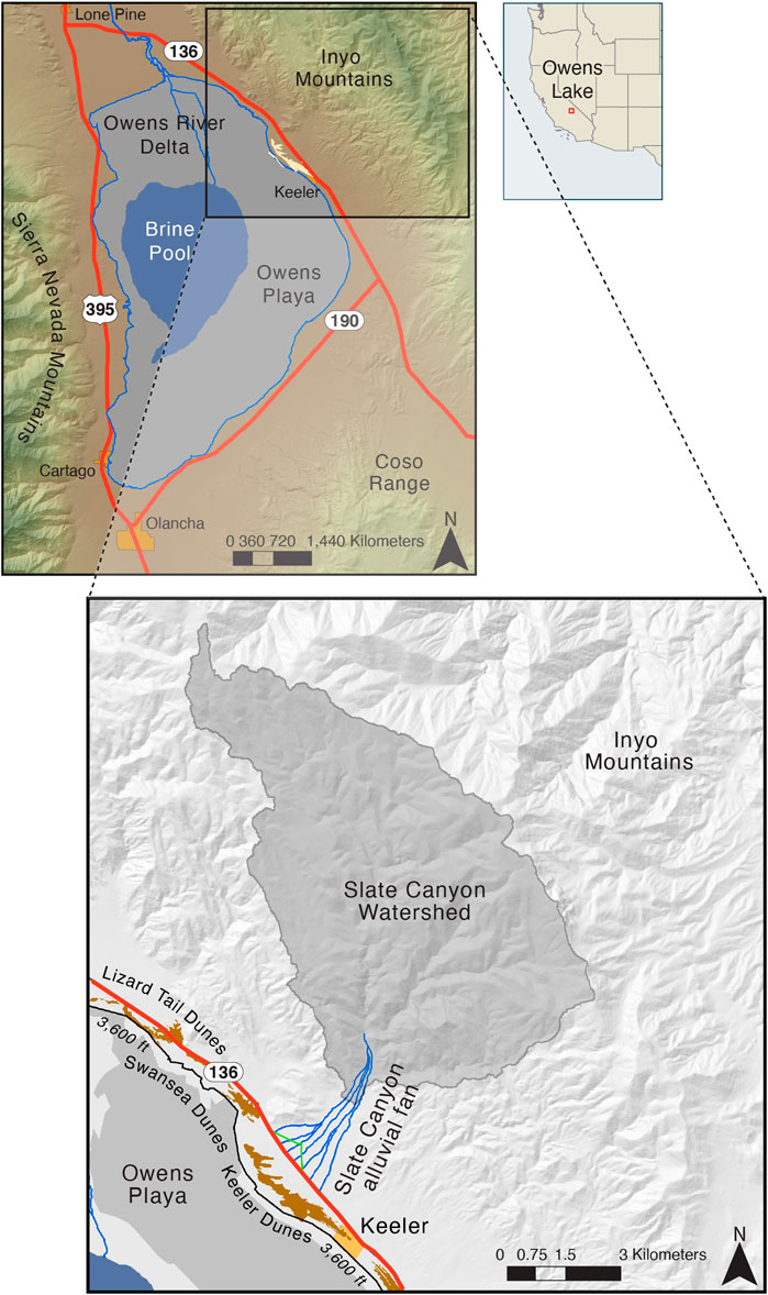
FIGURE 1. Vicinity map of Owens Lake, the Slate Canyon watershed, and the Keeler Dunes. Approximate outlines of modern dunes are shown in tan. The diversion berm system above State Highway 136 crosses the Fan near the toe at an approximate elevation of 3,750 ft (1,143 m) and is shown in green. The apex of the berm system is located at an approximate elevation of 3,850 ft (1,173 m). The watershed is located on the eastern side of Owens River Valley in the northeastern Inyo Mountains.

Aerial photographs and satellite images of the Keeler Dunes show that the dunes changed greatly from 1947 to present (Lancaster and McCarley-Holder, 2013). Sections of the dunes became destabilized leading to migration and expansion. Previous studies (Lancaster and McCarley-Holder, 2013; Lancaster et al., 2015) have implicated the desiccated Owens Lake playa as the source of material for this migration and growth and attribute changes in sediment availability from the playa to observed dune migration and morphogenesis. However, given the complex alluvial-aeolian interactions that inevitably occur in the vicinity of the Keeler Dunes, aeolian transport of playa sediment is not likely the only source of material contributing to dune growth and migration.

Playas have been commonly seen as the largest dust source in arid regions (e.g., Parajuli and Zender, 2017). However, observations of dust generation from the nearby eastern Mojave Desert and western Sonora Desert attribute relatively large contributions from proximate sources (i.e., alluvial fans and washes) and relatively small contributions from regional sources (i.e., desiccating pluvial lakes and playas) (Reheis and Kihl, 1995; Sweeney et al., 2013; Muhs et al., 2017). Likewise, assessments of potential emission by various desert landforms in the Namib desert (von Holdt et al., 2019), Lake Urmia (Ahmady-Birgani et al., 2018), and Owens (dry) Lake (Kolesar et al., 2022) also observed higher potential emissions from alluvial systems and related landforms compared to ephemeral lake systems. These studies call into question the relative importance of playa versus alluvial sources as material available for aeolian transport.

Investigations of alluvial fan behavior in the region have been focused on the Mojave Desert (McDonald et al., 2003; Miller et al., 2010), the western Owens River Valley (Danskin, 1998; Blair, 2001; Benn et al., 2006; Dühnforth et al., 2007; D’Arcy et al., 2017), and the White Mountains, north of the Inyo Mountain Range (Beaty, 1989; Hubert and Filipov, 1989; Osborn and Bevis, 2001). The lack of focus on the eastern Owens River Valley may be a function of local hydrology. Runoff from the Inyo Mountains does not provide much drinking water to adjacent jurisdictions, nor does it impact highly populated areas. However, studies of sediment yield in relation to annual mean precipitation suggest this area is of interest in terms of sediment contributions to the valley, as maximum sediment yield occurs when the effective annual precipitation is approximately 12 in (30.5 cm) (Langbein and Schumm, 1958; Schumm, 1977). This value is in the range of total annual rainfall expected for the Inyo Mountains (Danskin, 1998). Given the proximity to the Keeler Dunes and the potential for high sediment yield, the Slate Canyon and its watershed are important to consider for Keeler Dunes sediment origin.

In the case of the Keeler Dunes, two highway construction berms were constructed in 1954 and 1967 on the Slate Canyon alluvial fan directly upgradient of the dunes. The timing of berm construction coincides with observed destabilization and subsequent growth and migration of the Keeler Dunes. Construction of roadways and water diversion structures have a well-known impact on surface flows and sediment deposition (e.g., Jones et al., 2000; Phippen and Wohl, 2003). These construction activities have other secondary effects, including changes to the distribution of vegetation near the roadway (Schlesinger et al., 1989) and potential contributions to desertification by increasing resource fragmentation (Okin et al., 2009). Additionally, changes to runoff velocity and channel incision may cause changes to groundwater infiltration (Blainey and Pelletier, 2008). In the case of the Slate Canyon alluvial fan, a recent study by Richards et al. (2022) confirms that the diversion of flow caused by berm construction is likely the driving force behind observed changes in plant cover on the alluvial fan and on the Keeler Dunes. They conclude that these changes contributed to an estimated 4.4-fold increase in sand movement compared to the theoretical scenario of no vegetation changes (Richards et al., 2022).

The objectives of the current study are two-fold: 1) estimate the total amount of sediment that may have been yielded to the toe of the Slate Canyon alluvial fan, and 2) determine how the construction of the diversion berms affected the spatial distribution of sediment deposition at the fan toe and on the dunes. These questions will be investigated using several hydrologic and sediment transport models that are adapted to the Slate Canyon watershed to provide total estimates of transported material for several large-scale events. The estimates of sediment deposition under the berm and no-berm scenarios will support a more complete understanding of the balance between alluvial and playa sediment supply that contributed to the genesis and cause(s) of the destabilization and migration of the modern Keeler Dunes. This provides a case study as to how anthropogenic activities may impact the formation and morphogenesis of dune systems and adds to the ongoing discussion of the relative importance of alluvial vs. aeolian processes in shaping arid environments.

2 Materials and Methods

Hydrologic and hydraulic modeling was conducted to assess the potential watershed and fan sediment yield associated with the Slate Canyon alluvial fan (the Fan) and Keeler Dunes. Stream flows originating in the Slate Canyon watershed were estimated using a hydrologic model based on hourly precipitation records at neighboring gages. The resulting Slate Canyon alluvial fan flows were used in a two-dimensional hydraulic model of the alluvial fan. This model applied multiple sediment transport and yield methods to assess the volume of material that is moved from the alluvial fan hydrographic apex, downgradient toward the Keeler Dunes area. This case study of the peak event of record (6 December 1966) is used to investigate the possible fate of sediment deposition on the fan.

2.1 Hydrologic Modeling

The Hydrological Simulation Program–Fortran (HSPF) package was selected to model the hydrologic characteristics associated with the Inyo Mountains. The HSPF model of the Slate Canyon watershed was developed using the Environmental Protection Agency’s Better Assessment Science Integrating Point and Nonpoint Sources (BASINS) tool, which is a “multipurpose environmental analysis system designed for use by regional, state, and local agencies in performing watershed and water-quality-based studies” (United States Environmental Protection Agency, 2019). The modeling package incorporates Geographic Information System (GIS) data coverages, including United States Geological Survey (USGS) topographic, NLCD (National Land Cover Database) land use, and NRCS (National Resources Conservation Service) soils mapping to create an HSPF model file. For the Slate Canyon model, pervious land segments (perlands) were developed using soils and land cover.

A digital elevation model (DEM) of the Inyo Mountains was used within the BASINS program to delineate the subbasins’ tributary to the alluvial fan hydrographic apex. The USGS DEM is a terrain elevation data set in a digital raster form with coverage of the entire contiguous United States at a 300 m × 300 m cell size. The resulting Slate Canyon subbasins are shown in Supplementary Figure S1. The BASINS program assigned ID numbers to each of the subbasins. Based on the delineations, the total area of the subbasins used to generate the flow hydrograph at the Fan hydrographic apex was 21.5 mi² (55.7 km²). Subbasin 30 was determined to contribute flow to a separate, smaller flow path and was not included in the hydrologic calculations.

The HSPF model used hourly precipitation data from valley floor gages, adjusted for elevation, along with temperature, and evapotranspiration data to estimate a continuous representation of the hydrologic processes and surface water flows from Slate Canyon and discharging to the Fan hydrographic apex. The available meteorological data for precipitation, air temperature, and evapotranspiration allowed the Slate Canyon HSPF model to produce a flow hydrograph simulation from October 1948 to May 2013.

2.1.1 Land Use

Land use is an important factor for all hydrologic modeling exercises. For the development of the Slate Canyon HSPF model, the National Land Cover Database 2001 (LaMotte, 2016) was used to delineate the multiple land uses and vegetation covers in the Slate Canyon watershed. The NLCD is a 16-class cover classification scheme that has been applied consistently across all 50 United States and Puerto Rico at a spatial resolution of 30 m (Homer et al., 2007). As shown in Supplementary Table S1, most of the study area consists of scrub/shrub land (class 52), with evergreen forests (class 42) in the upper watershed, comprising the next largest land cover classification. These two land classifications make up over 99 percent of the study area.

2.1.2 Soils

The initial hydrologic parameters based on soil characteristics were estimated based on the State Soil Geographic (STATSGO) database (Soil Survey Staff and National Resources Conservation Service, 2022). Supplementary Figure S2 illustrates the distribution of the various soil types in the study area. The STATSGO database includes hydrologic soil parameters such as permeability, water storage capacity, and horizon depth, which influence the HSPF parameters: LZSN (lower zone nominal soil moisture storage), UZSN (nominal upper zone soil moisture storage), and INFILT (index to mean soil infiltration rate). The soils classifications (Supplementary Table S2) generally traverse the study area in bands. In the HSPF model development, this fact provided the ability to assign meteorological data based on elevation bands that generally corresponded to the soils.

2.1.3 Meteorology

Meteorological data files were prepared for the Slate Canyon HSPF model. These covered the October 1948 to May 2013 period (65 years, 23,600 h). There are no long-term recording weather stations in the Slate Canyon study area. The nearest weather stations with a sufficient period of record (United States Department of the Interior Geological Survey, 1982) were in the towns of Independence and Bishop, and included: hourly precipitation, hourly air temperature, hourly dew point, hourly wind speed, hourly solar radiation, and daily potential evapotranspiration.

The most important meteorological parameters for the HSPF model approach used for the Slate Canyon were hourly precipitation and air temperature data. The air temperature data provided discrimination between snow and rain by elevation zone. The files for dew point, wind speed, and solar radiation were primarily used to determine spring snowmelt. Spring snowmelt produces significant flows at the Fan hydrographic apex only in wet years and does not cause the large floods that can move sediment to the fan toe.

The original hourly precipitation data at Independence contained many missing hourly precipitation events, mostly in earlier years, such as during the large storm events on 18 November 1950; 6 December 1966; and 25 January 1969. These storms likely produced flow at the Slate Canyon Fan hydrographic apex and therefore are important to include in the analysis. Other meteorological data recorded at Bishop (a nearby station at similar elevation), Cottonwood (southwest of the Owens Lake playa), and Keeler (east of the Owens Lake playa) were used to supplement the Independence records. Air temperature data showed that snow or rain discrimination (the snowline) fluctuated widely in these events. Snowfall and snowpack water retention were also important for some other flood events (e.g., 8 February 1978, and 4 March 1991).

Independence (and Bishop) also had daily precipitation records, which were more complete than the hourly precipitation records. The hourly precipitation instrument record was subject to missing data due to equipment failures, summer/fall inactive status, and snow capping. Independence (and Bishop) also had daily snowfall files.

Daily precipitation records at Independence were used to define periods when hourly precipitation was missing but should have occurred. For these occurrences, substitutions were made using the Bishop, Cottonwood, or Keeler records. Summer/fall monsoonal cloudbursts exhibited by the daily record at Independence were distributed hourly using the National Oceanic and Atmospheric Administration (NOAA) Atlas 14 statistical distributions. Nearly all cloudburst rainfall occurred in 1 hour.

The Independence precipitation data reflect recorded values on the valley floor at an approximate elevation of 4,000 ft (1,219 m). The Slate Canyon study areas extend to elevations above 9,000 ft (2,743 m). The orographic impact of the mountains results in a higher precipitation total in the upper watershed. The presence of conifer forest above 7,000 ft (2,134 m) elevation indicates higher annual precipitation [over 15 in (38 cm) from PRISM (Parameter-elevation Regressions on Independent Slopes Model) mapping, see Supplementary Figure S3]. To account for the increased precipitation at higher elevations, a multiplier was used on the Independence precipitation data. The multiplier ranged from 1.1 for the lower elevation to over 2.0 in the upper areas.

Air temperature was the most important discriminator of snowfall from rain. Discrimination of snow from rain by elevation zone in the Slate Canyon watershed was essential to meaningful simulation of flood runoff. Air temperature was based on maximum-minimum air temperature data from Independence, converted to hourly using a sinusoidal distribution. This estimate was corrected during precipitation events when hourly air temperature data were available at Bishop (1982–2013). For earlier years, the air temperature record was revised to be consistent with snow observations. Solar radiation data were estimated from theoretical clear sky solar, corrected for precipitation days. Solar radiation data were most important for spring snowmelt simulation of high elevation snowpacks (typically over 7,000 ft (2,134 m) in the Inyo Mountains).

Dew point data were estimated from minimum temperature, precipitation, and recent CIMIS (California Irrigation Management Information System) data at the Owens Lake North station. Wind speeds were estimated from the Owens Lake North CIMIS station data. Dew point and wind speed data have relatively minor effects on floods, except those that had a snowmelt component.

2.1.4 Channel Transmission Losses

USGS Water Resources data of southwest desert stream-flow records show that channel and fan losses to groundwater are important in determining surface flows at a fan toe. The HSPF model did not include a methodology for determining alluvial channel transmission losses.

From aerial photography and field observations, the Slate Canyon alluvial channel upstream of the Fan hydrographic apex was estimated as 1.24 mi (2 km) in length, with a bed width of 50–200 ft (15.2–61 m), a maximum area of 110 ac (445,154 m²), and with bed material of coarse sand and gravel. HSPF hourly flows at the apex were adjusted to account for upstream channel transmission losses using the methodology of Cataldo et al. (2010). For the Slate Canyon 2 km reach, their power equation showed losses of:

• 40 percent for 20 cfs (0.56 m³/s) (lower limit of equation)

• 20 percent for 100 cfs (2.83 m³/s)

• 11 percent for 1,000 cfs (28.3 m³/s)

• 6 percent for 10,000 cfs (283 m³/s)

2.1.5 Streamflow Estimates

There are no known recording precipitation or stream flow gages located within the Slate Canyon watershed. Neighboring watersheds with similar hydrologic characteristics also did not have recording gages. Without available recorded flow data, the HSPF model could not be calibrated. To validate that the model provides representative results, the peak flow analysis results were compared to peak flows using other standard methods: USGS Regional Regression model (Waananen and Crippen, 1977) and HEC-1 (Blood and Humphrey, 1990). The USGS results are based on regional regression equations developed from an analysis of existing flow gages in the region.

2.2 Sediment Yield

In this study, watershed sediment yield was calculated using two methods: 1) the Modified Universal Soil Loss Equation (MUSLE) (Mussetter et al., 1994), and 2) United States Army Corps of Engineers Los Angeles District Method (Gatwood et al., 2000). The latter will hereafter be referred to as the USACE method.

2.2.1 Modified Universal Soil Loss Equation

Both the Albuquerque Metropolitan Flood Control Authority (AMAFCA) (Mussetter et al., 1994) and Jackson et al. (1986) indicate that MUSLE runoff energy coefficients can be adequately adjusted to represent watersheds outside of the original study area. MUSLE is more applicable to arid environments than its predecessor, Universal Soil Loss Equation (USLE), where the runoff factor replaces the rainfall energy factor (Simons and Sentürk, 1992). For the purposes of the present study, it is recognized that MUSLE is most generally applicable as a wash load (i.e., D50 > 1 mm) estimation method (Simons and Sentürk, 1992).

The MUSLE method (Mussetter et al., 1994) utilizes an empirical equation (Eq. 1) that considers storm energy runoff (Rw), soil erodibility (K), topographic relief (LS), vegetative cover (C), and a conservation practice factor (P).

$Ys=Rw\cdot K\cdot LS\cdot C\cdot P(1)$

where, Ys is sediment yield in tons, and Rw is storm energy runoff in the form:

$Rw= \alpha {\left(VQ\right)}^{\beta }(2)$

where V is the runoff volume for the storm in acre-feet and Q is in cfs and represents the peak discharge of the storm as derived from the HSPF modeling. The values of Q are reported in Table 2. For the calculation of Rw, the values of α and β can be adjusted based on AMAFCA (Mussetter et al., 1994) and Jackson et al. (1986) to account for the unique runoff energy coefficients of the study watershed; however, for this analysis they are left at the standard values of 95 and 0.56, respectively, in the absence of documented calibration.

The vegetative cover value, C, was based on a review of available aerial photography of the watershed (Google Earth, 3 June 2004). The watershed ranges in vegetative canopy and cover from herbaceous desert plants to alpine-type assemblages. A mix of covers based on a random sample of watershed subareas was used to ultimately develop the value of C = 0.1.

Soil erodibility, K, was given a value for soils consistent with gravely loamy sand (K = 0.10).

Topographic relief was calculated using the following equation:

$LS={\left(\frac{\lambda }{72.6}\right)}^n\ast \left(0.065+0.454\ast S+0.0065S^2\right)(3)$

where λ is the slope length (13,705 ft/4,177 m), S is the percent slope (10%), and n is based on the percent slope (n = 0.5 for slope ≥ 5%). The topographic relief value LS is 16.1.

The conservation practice factor (P) is one (1) because the Slate Canyon alluvial fan has no manmade erosion resistance facility.

2.2.2 USACE Los Angeles District Method for Prediction of Debris Yield

The USACE method considers unit peak runoff, tributary topography, drainage area, and potential fire impacts. The equation for debris yield (DY) for a hydrologic event for the Slate Canyon watershed is given in (Eq. 4):

$Log\left(DY\right)=0.94Log\left(Qu\right)+0.32Log\left(RR\right)+0.14Log\left(A\right)+0.17FF(4)$

where, DY is debris yield in yd³/mi², Qu is the unit area discharge in cfs/mi², RR is the relief ratio or slope in ft/mi, A is the drainage area (acres), and FF is the fire factor. RR is 2,170 ft/mi (411 m/km). Qu was determined by dividing the peak discharge of the storm (Q) in cfs by the drainage area. A is 16,256 acres (25.4 mi²/65.8 km²); the size of the Slate Canyon watershed. FF is three (3), the value for a watershed, such as the Slate Canyon watershed, in which wildfire plays an insignificant role in debris product (Gatwood et al., 2000). A density of 1.7 g/cm³ was assumed when converting from volume to mass.

2.3 Fan Sediment Yield

The FLO-2D numerical model is designed to be utilized for delineating flood hazards or designing flood mitigation. The model is made up of a series of computational parameter modules that separate an analysis into component parts including overland flow and other physical features. The model is described in depth elsewhere (FLO-2D Software Inc., 2021), and briefly summarized here.

2.3.1 FLO-2D Model Description

In FLO-2D modeling, the equations of motion in two dimensions contain a mass and momentum balance and take the form:

$\frac{\partial \text{h}}{\partial \text{t}}+\frac{\partial {\text{hv}}_{\text{x}}}{\partial \text{x}}+\frac{\partial {\text{hv}}_{\text{y}}}{\partial \text{y}}=\text{i}(5)$

${\text{S}}_{\text{fx}}={\text{S}}_{\text{ox}-}\frac{\partial \text{h}}{\partial \text{x}}-\frac{{\text{v}}_{\text{x}}\partial {\text{v}}_{\text{x}}}{\partial \text{x}}-\frac{{\text{v}}_{\text{y}}\partial {\text{v}}_{\text{x}}}{\text{g}\partial \text{y}}-\frac{\partial {\text{v}}_{\text{x}}}{\text{g}\partial \text{t}}(6)$

${\text{S}}_{\text{fy}}={\text{S}}_{\text{oy}-}\frac{\partial \text{h}}{\partial \text{y}}-\frac{{\text{v}}_{\text{y}}\partial {\text{v}}_{\text{y}}}{\partial \text{y}}-\frac{{\text{v}}_{\text{x}}\partial {\text{v}}_{\text{y}}}{\text{g}\partial \text{y}}-\frac{\partial {\text{v}}_{\text{y}}}{\text{g}\partial \text{t}}(7)$

where subscripts x and y represent the two component directions, i is input (e.g., precipitation), and S_o is the bed slope. A diffusive wave approximation neglects the last three terms on the right-hand side of the latter two equations. In the case of the diffusive wave approximation, the accelerations are ignored, but pressure gradients participate in the balance of momentum and balance of bed slope and bed friction, leaving:

$\frac{\partial \text{h}}{\partial \text{x}}={\text{S}}_{\text{ox}-}{\text{S}}_{\text{fx}}(8)$

$\frac{\partial \text{h}}{\partial \text{y}}={\text{S}}_{\text{oy}-}{\text{S}}_{\text{fy}}(9)$

This is an important difference compared with a one-dimensional model such as HEC-RAS (Hydrologic Engineering Center’s River Analysis System). The diffusion model is not restricted to channels, and the time-dependent components allow for discharge to vary during a simulation. Unlike 1D HEC-RAS, FLO-2D uses a complex set of equations, which require detailed numerical methods to solve them. In the case of FLO-2D, the differential form of equations are solved with a central, explicit, finite difference scheme such that the discharge across one grid element boundary into another is accomplished one element at a time. The uniform grid elements that comprise the model are used to calculate discharge in eight flow directions: four compass directions and four compass diagonals.

Numerical computations begin in each grid element by estimating the depth of flow at the boundary between two adjacent elements. The equations of motion are applied to determine the velocity one direction at a time for all eight flow directions of a given element. Discharge across the element boundary is calculated by multiplying velocity with the cross-sectional flow area. Once all four boundary element discharges have been calculated, the change in volume for the individual element can be calculated by multiplying the sum of discharges by the time step. The change in water depth can then be determined by dividing the change in volume by the element surface area. Volume conservation is checked at every time step in every computational element to provide a check of accuracy and as a tool to determine if user-selected parameters are properly exercised. One of the most important computational components of a finite-element numerical scheme is the numerical stability criteria. In the case of FLO-2D, the stability is variable and is based on the Courant-Friedrichs-Lewy (Courant et al., 1967) condition and time stepping increments or decrements to maintain model stability.

2.3.2 FLO-2D Model Application

For the Slate Canyon alluvial fan and vicinity, one DEM for an existing-condition scenario and another DEM for a no-berm scenario were obtained from LiDAR data acquired by Photo Science, Inc. in August 2012. The DEMs have a pixel resolution of 1 m. The no-berm scenario DEM (not shown) is the same as the existing-condition DEM (Figure 2) except in the vicinity of the Caltrans berm up-Fan of State Highway 136. The berm feature was digitally removed to generate a data set representative of historical topographic conditions on the lower Fan. For the upper third of the Fan, where no LiDAR data is available, model topography was developed by up-sampling 3 m resolution InterMap data to a 20 ft (6.1 m) pixel resolution DEM. The resulting model topography of the entire study area is shown in Figure 2 for the existing berm scenario.

FIGURE 2

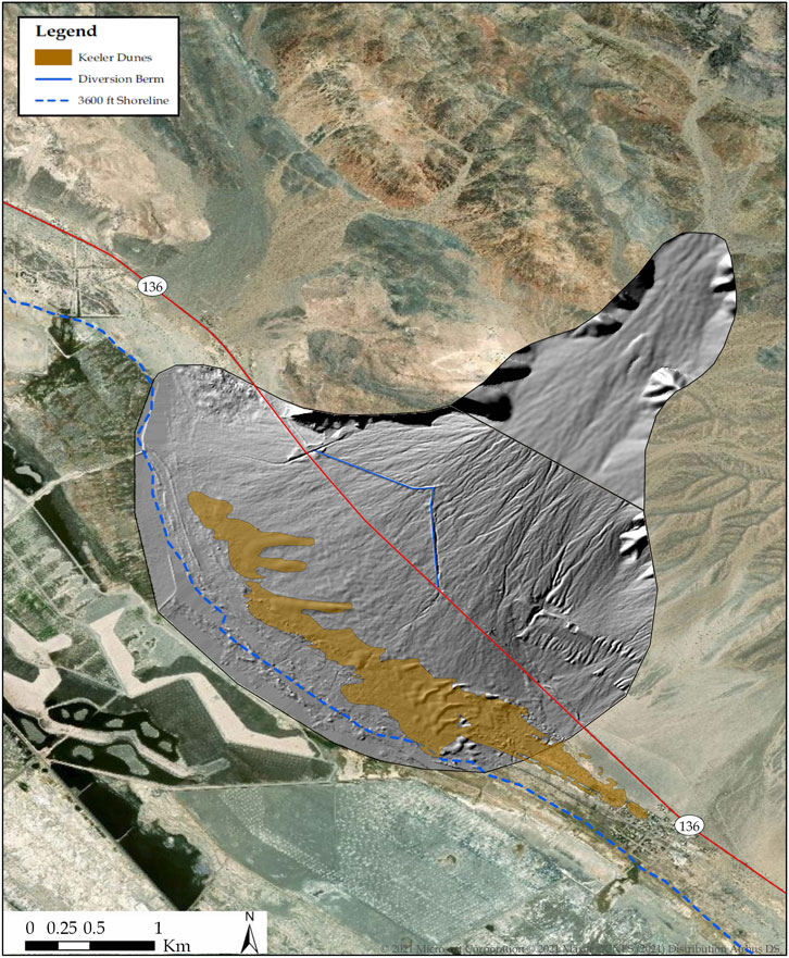
FIGURE 2. Slate Canyon Alluvial Fan two-dimensional modeling area DEM. The model is comprised of the Fan below the hydrographic apex to Keeler Dunes. The berm system is highlighted (blue line) and the separation between the upper and lower fan sections is shown. The Keeler Dunes (brown shaded area), the historic shoreline (blue dashed line), and State Highway 136 (red line) are all shown.

FLO-2D modeling is broken into two model areas and two conditions. The first model area covers the upper half of the Fan, separated approximately at the up-Fan limit of aeolian sand depositions, while the second extends from the first model boundary down to, and including, the Keeler Dunes. The reason for breaking the model into two components was to limit run times; join the two different topographic resolutions, described above; and reduce model grid size (increase model topographic resolution). Additionally, in the no-berm condition, described below, the changes to topography can be kept separate from the upper Fan without disturbing the flow distributions of the upper model. The two models are coupled at the models’ boundaries by distribution of flow between the respective in- and out-flow locations (Jaffe, 2008). Finally, analysis sections, described below, are added to the model to provide FLO-2D model output as input to model sediment transport potential at these same locations.

For all model runs it was assumed that no rainfall was present on the Fan, as local and regional orographic effects limit the amount of direct rainfall to the Fan.

2.4 Sediment Sampling

Sediment data were collected from nine sites on 11 June 2013 (Figure 3). One sample was taken near the Fan topographic apex (APEX), two on the upper Fan (SC6, SC4), one in the transition zone (SC4.5), two below the berm (SC5, SC1), one in the Fan channel (SC2), and two other samples (SC4.9, SC4.8) just up-Fan of Caltrans diversion berm. For each collection site, three samples were taken at approximately 1 ft (30.5 cm) depth in the active or recently active bed. The three samples at each location were mixed in situ, and the mix was resampled in the field following ASTM D6913. The sieve analysis was conducted by IAS Labs. Sieve sizes were standard U.S. mesh sizes greater than sieve #200. Maximum mesh size was dependent on maximum particle size at the sampling location, which for all locations was 1 in (2.54 cm). The goal of the analysis was to gain a statistical representation of the size distribution of soil on the Fan surface to be used in the SAM modeling (Section 2.5).

FIGURE 3

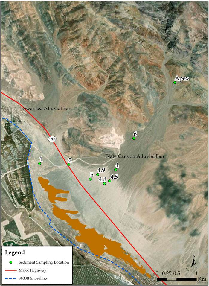
FIGURE 3. Sediment sampling location on Slate Canyon alluvial fan. Samples were taken on 11 June 2013. For each collection site, three samples were taken at approximately 1 ft (30.5 cm) depth in the active or recently active bed.

2.5 Sediment Transport Potential

Sediment transport potential at the Caltrans berm was estimated in this study using the USACE SAM numerical model. The SAM Sediment Model is an integrated system of programs developed through the Flood Damage Reduction and Stream Restoration Research Program to aid in the analyses associated with designing, operating and maintaining flood control channels and stream restoration projects (Thomas et al., 2002). To account for highly localized fluctuations in grainsize distribution, local sediment data (Section 2.4) were entered using average sediment values. SAM model runs were conducted at 10 analysis sections defined in the FLO-2D model. These analysis sections provide FLO-2D output to be used directly as input to the SAM modeling. The transport potential is compared to watershed sediment yield to suggest if the Fan is a source of sediment to Owens Lake, or a sink for sediments delivered to the Fan for the Slate Canyon Watershed.

Sediment transport equations used in all SAM modeling were chosen with the assistance of SAM’s SAM.AID subroutine and Yang and Huang (2001). The SAM.AID subroutine determines the most representative transport function based on the hydraulic parameters and presents finer data for each subreach by comparing model data with the results of 20 peer-reviewed sediment transport studies (Thomas et al., 2002). This case-by-case transport equation selection is more likely to provide a robust representation of channel sediment transport than choosing an individual transport equation for all reaches. The Yang and Huang (2001) equation was found to be representative of the study area.

2.5.1 Transport Capacity

Using available USGS DEM data for the Slate Canyon area above the alluvial fan, a HEC-RAS hydraulic model was developed (Supplementary Figure S4). Cross-sections cut from the DEM surface were edited to include defined channels based on aerial photography. The channel widths were estimated from the aerials and each channel was assumed to have a depth of 2 ft (61 cm) below the DEM elevation.

3 Results

The modeling effort described herein included two separate conditions: the existing condition in the lower fan model with the current Caltrans berm system in place, and a hypothetical condition where the berm system is removed. The no-berm model condition is representative of the lower Fan prior to the construction of the berm.

3.1 Hydrologic Modeling

Hydrologic modeling was performed using the HSPF package to estimate how precipitation in the 25.4 mi² (65.8 km²) Slate Canyon watershed translates to surface flow. Based on the HSPF model results for a simulation period of October 1948 to May 2013, a flood frequency analysis was conducted. The peak flow rates for various return periods are shown in Table 1. Within the table, the HSPF flows are a direct result based on modeled annual peaks. The HSPF-Loss Adjusted results represent the peak flows at the hydrographic apex with channel losses accounted for using the methods outlined in Section 2.1.4. At flows over 25 years, the volume of moisture in the channel and underlying ground restricts infiltration losses.

TABLE 1

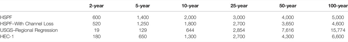
TABLE 1. Peak Flow Comparisons at Slate Canyon Alluvial Fan Hydrographic Apex (expressed in cfs).

There are no known recording precipitation or stream flow gages located within the Slate Canyon watershed. Neighboring watersheds with similar hydrologic characteristics also did not have recording gages. Without available recorded flow data, the HSPF model could not be calibrated. Therefore, the peak flow analysis results in Table 1 were compared to peak flows resulting using other standard methods: USGS Regional Regression model (Waananen and Crippen, 1977) and HEC-1 (Blood and Humphrey, 1990). The USGS Regional Regression model results are based on regional regression equations developed from an analysis of existing flow gages in the general region (Waananen and Crippen, 1977). The HEC-1 flows are from a previous modeling effort investigating cloudburst flows using a single design storm, not a continuous model like the HSPF (Blood and Humphrey, 1990).

The USGS Regional Regression model (Waananen and Crippen, 1977) showed lower peak flows compared to the HSPF model for recurrence intervals of 25 years or less. This difference was attributed to alluvial fan infiltration losses, which were not incorporated in the HSPF model. These comparisons are imperfect since the HSPF events were nearly all winter rain/snowmelt events while the USGS and HEC-1 results were summer/fall cloudburst events. However, they provide information as to the reasonableness of the HSPF results for the Slate Canyon alluvial fan.

The Slate Canyon HSPF modeling effort produced a continuous flow time series. Due to the long time periods with no recorded precipitation, the HSPF modeling resulted in long periods with no flows. Subsequent hydraulic modeling, described below, was concerned only with flows capable of transporting sediment, so the subset of the long-term hydrograph (1948–2013) used for this study was concatenated removing all flows under 500 cfs (14.16 m³/s). Flows under 500 cfs at the Fan hydrographic apex were determined to not have the energy for sediment transport. The resulting hydrograph in Figure 4 represents approximately 0.06% of the total simulation period (∼320 h over 64 years).

FIGURE 4

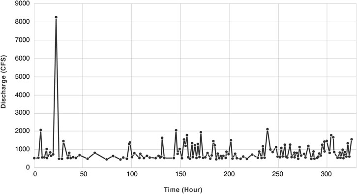
FIGURE 4. Hydrograph subset from HSPF modeling. The linearized long-term hydrograph (64 years) derived from HSPF modeling is shown for a subset (320 h) of the modeled time. Discharges smaller than 500 cfs (14.16 m³/s) were removed to facilitate an understanding of events capable of sediment transport.

HSPF results showed the Slate Canyon mean annual runoff as 6,000 ac-ft/7,400,880 m³ (5 in/12.7 cm) at the Fan topographic apex. There was a marked difference between dry and wet year runoff from near zero to 20 in/50.8 cm (1969 precipitation year). Taking into consideration the 67% flow loss across the alluvial fan (valley fill), the estimated volume of flow potentially reaching the playa is 4,000 ac-ft/4,933,920 m³. The maximum simulated flood event was 6 December 1966, at 8,861 cfs (251 m³/s). About a third of the events more frequent than the 2-year return period event are near zero.

The loss-adjusted continuous flow time series generated by the HSPF program was used as an input flow source for the FLO-2D sediment transport model of the alluvial fan.

3.2 Sediment Yield at Fan Hydrographic Apex

At present, no direct measurement of sediment yield for the Slate Canyon watershed is available for the Slate Canyon alluvial fan. In this study, watershed sediment yield was calculated using two methods: 1) the Modified Universal Soil Loss Equation (MUSLE) (Mussetter et al., 1994), and 2) United States Army Corps of Engineers Los Angeles District method (Gatwood et al., 2000). Neither sediment yield method was originally intended for application in California high-desert environments such as the Owens River Valley. The MUSLE method was originally developed for experimental watersheds in Texas and Nebraska (Mussetter et al., 1994), and the USACE method (Tatum, 1963) was originally developed for coastal Southern California watersheds (Gatwood et al., 2000), both of which are geologically and climatologically different from the study area in this analysis. In both cases, however, the methods accounted for the differences in watershed parameters used in the calculations.

The estimated sediment yield for the individual storms in the hydrologic time series using both the MUSLE and USACE methods are shown in Table 2. The MUSLE and USACE methodologies produce a range of watershed debris yield ranging from 2,976,223 US tons/2,699,984 t (MUSLE) to 3,951,561 US tons/3,584,796 t (USACE) tons for all events greater than 1,500 cfs (42.48 m³/s) at the Fan topographic apex over the period of record (1948–2013), respectively. Moreover, the difference in results is Δ ≈ 975,000 US tons (884,505 t), or a 25% difference for all events greater than 1,500 cfs (42.48 m³/s) at the Fan hydrographic apex over the period of record. Such differences are not uncommon between the two methods, and the actual value is expected to range between that predicted by these two methodologies during a given runoff year. It is important to recognize these methods are an attempt to represent the bounds in which the actual watershed sediment yield lies. The paucity of data in the watershed creates a level of uncertainty with the present analysis, and the use of multiple methods to arrive at a range is more likely to produce representative results than a single method.

TABLE 2

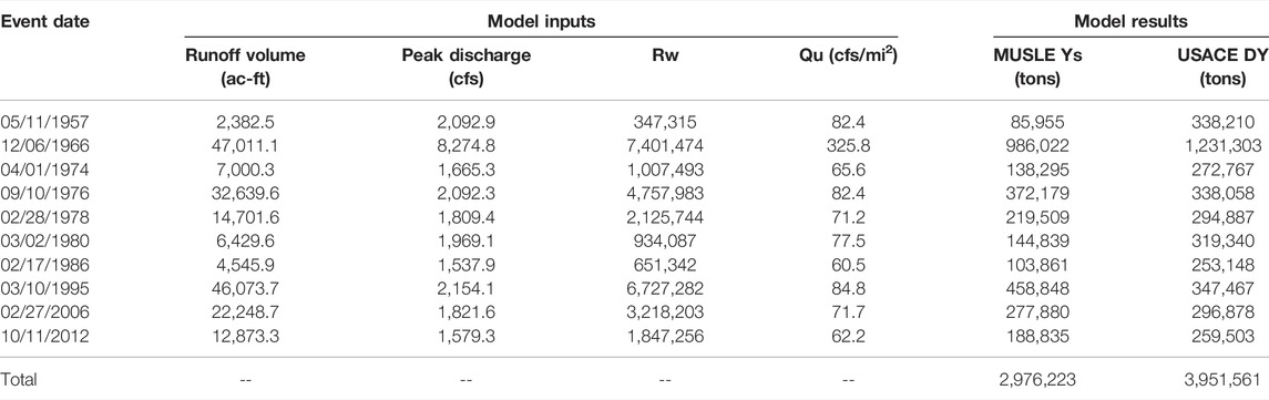
TABLE 2. Estimates of Watershed Sediment Yield at the Fan Hydrographic Apex, by Event, using MUSLE and USACE methods. Events were days during which the flow was greater than 1,500 cfs during the periods from 1948 to 2013. The area of the Slate Canyon Watershed is 25.4 mi².

The maximum event of record occurred on 6 December 1966. For the December 1966 event, the debris production estimated by the USACE method is approximately 48,500 tons/mi² (16,987,900 kg/km²). This event is used as a case study in the following sections to determine the potential amount of sediment transported by the Fan and the distribution of sediment in the berm and no-berm scenarios.

3.3 Hydraulics Modeling

tThe loss-adjusted, continuous flow time series generated by the HSPF model (Figure 2) was used as inputs to FLO-2D to calculate the Fan sediment yield on the lower portion of the Slate Canyon alluvial fan occupied by the Keeler Dunes. Two scenarios were considered for modeling: berm and no-berm. These two scenarios are referring to water diversion berms that were constructed by CalTrans in 1954 and 1967 upgradient of State Highway 136. The purpose of comparing the two scenarios is to estimate the impact the berm system has on surface flows and sediment delivery to Keeler Dunes below the current location of State Highway 136. A short-run, peak-event linearized hydrograph (6 December 1966) was used to generate model maximum inundation output analysis.

Panels A through D of Figure 5 clearly show how the outflow of the upper Fan model provided for the inflow of the lower Fan models. The importance of the feeder channels for directing overall flow onto the Fan can also be observed such that the existing hydraulic conditions are observed to concentrate in the larger, more incised channels. The flow patterns appear to follow the more incised channels and generally match the flow pattern shown in the output of the FLO-2D numerical model runs. The maximum velocities and depths predicted on the upper Slate Canyon Fan for both the existing and no-berm scenarios are presented in Figure 5, respectively, for the maximum event of record on 6 December 1966. Both the existing berm and no-berm scenario velocities and depths range from 0.0 to >12.0 ft/s (3.66 m/s) and 0.0 to >7.0 feet (2.13 m), respectively.

FIGURE 5

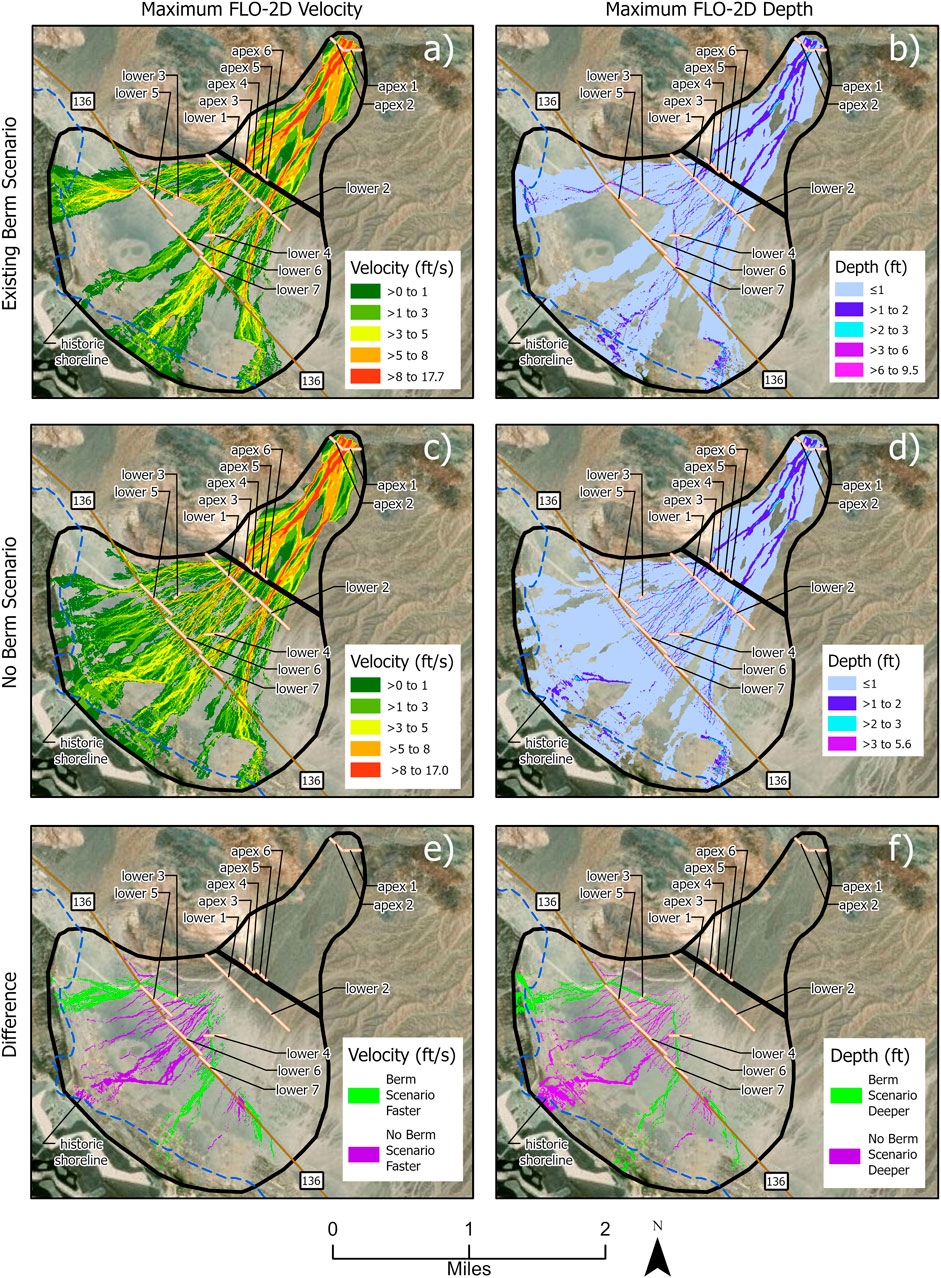
FIGURE 5. FLO-2D modeling results for peak event of record (12/6/1966). The maximum flow velocity (A,C) and maximum depth (B,D) are shown for the existing and no-berm modeling scenarios. The difference in velocity and depth between scenarios is shown in panels (E,F), respectively.

The distribution of surface flow on the Fan in the existing with berm condition suggests that the primary result of the presence of the berm is to shadow some portions of the lower Fan from up-Fan runoff. There are two primary shadowed locations of the Fan (Figures 5A,B): an area shadowed by the north arm of the berm represented by analysis section “lower 5” and the north half of analysis section “lower 6”, and a small portion of the southern half of analysis section “lower 6”. Velocities are highest in the deeper flowing distributary channels and along the upstream side of the berm. As is expected for alluvial fan surfaces, velocity decreases in the down-fan direction, which is most clearly observed down-fan of analysis sections “lower 1” and “lower 2”. Likewise, the greatest depths are observed in the most incised channels and along the upstream side of the berm. The latter depths are controlled by backwatering at the berm.

In the no-berm condition (Figures 5C,D) the flow patterns are largely the same as the berm condition, except for the shadowed areas that are now largely available to surface flows and the area down-fan of “lower 7,” which receives no surface flows. The differences between the berm and no-berm conditions are shown in Figures 5E,F. The figure shows that fan flows are deeper and faster around the berm ends (green) in the berm scenario, while the area down slope of the diversion berms is faster and deeper in the no-berm scenario (purple). This is the expected result, except for some portions of the berm scenario that experience overtopping of the berm system and therefore experience flows down slope of the berm.

Model results clearly show the importance of the feeder channels for directing overall flow on the Fan. Existing condition flows are observed concentrating in the larger, more incised channels, particularly compared with the topography. The model results also indicate that, when present, the berm system diverts sediment-laden flows away from some portions of the down-fan Keeler Dunes area. Yet for events with discharge magnitudes on par with the 6 December 1966 event, the area down-fan of the southern portion of the berm system would be inundated by overtopping of the berm. It is not presently clear what topographic apex discharge magnitude will result in overtopping of the berm system, but the extensive inundation during the 6 December 1966 event suggests that the threshold for overtopping the berm is less than the discharge observed during the peak event of record.

The analysis sections shown in Figure 5 were selected to extend across primary flow paths on the Fan. Detailed, time-dependent hydraulic model results are output at each section to serve as the hydraulic input for the SAM modeling (discussed in Section 3.4). Therefore, SAM modeling proceeds at locations where Fan hydraulic behavior is indicative of primary sediment transport pathways.

3.4 Sediment Yield on Fan Surface

Sediment transport potential at the Caltrans berm was estimated in this study using the USACE SAM numerical model. SAM combines the hydraulic information and the bed material gradation information to compute the sediment transport capacity for a given channel or floodplain hydraulic cross-section for a given discharge at a single point in time or for a series of discrete hydraulic discharges. Several sediment transport functions are available for this analysis and SAM provides guidance to assist in selecting the most appropriate sediment transport equation.

3.4.1 Sediment Sampling

Sediment sampling was conducted to characterize the sediment of the Fan surface, and by extension the material that was transported during discharge events. The sediment sampling locations are shown in Figure 3, and the grain size distribution at each sample location is shown in Figure 6. The average gradation curve determined from these samples (Supplementary Figure S5) is used as an input to the sediment transport potential model (SAM model).

FIGURE 6

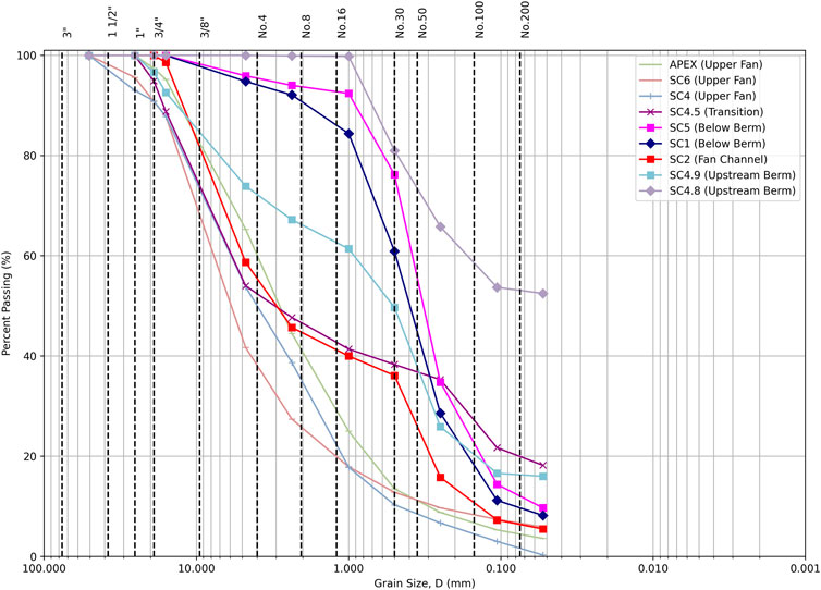
FIGURE 6. Grain size distribution for sediment samples. Grain size distribution is based on ASTM D6913 for US mesh sizes greater than sieve #200. Sample locations were from distinct regions of the Slate Canyon Fan. The upper Fan is represented by samples Apex, SC6, and SC4. The transition zone is represented by sample SC4.5. The area of primary aeolian deposits that exists below the water diversion berm is represented by samples SC1 and SC5. The distinct incised channels that are present on the Fan are represented by sample SC2. Samples SC4.8 and SC4.9 are taken upstream of the Caltrans berm. Aeolian deposits are centered around Sieve #16, or approximately 1 mm.

The grain size distribution of the upper Fan sediments (samples APEX, SC4 and SC6) is broader and more evenly distributed between the sieve sizes compared to samples from other areas. The average D₅₀ for the three upper Fan sediment samples is 4.236 mm (D_50,Apex = 2.441 mm, D_{50, SC4} = 3.257 mm, and D_50,SC6 = 3.500 mm) and the average composition of fines (smaller than sieve No. 200, approximately 0.075 mm diameter) is 3.3%. Below the berm (samples SC1 and SC5), the grain size distribution is more uniform compared to the samples in the upper fan. The average D₅₀ for samples SC1 and SC5 is 0.374 mm (D_50,SC1 = 0.416 mm and D_50,SC5 = 0.342 mm), which is smaller than the D₅₀ of the upper Fan sediments. Similarly, the fine percentage of the below the berm samples (SC1 and SC5) is higher (average = 9%) compared to the upper Fan sediments.

In addition to the upper Fan and the below the berm samples, there are four more samples from different areas of the fan. Sample SC2 was taken from an incised Fan channel diverted to the northwest by the Caltrans berm. This sample has a D₅₀ of 0.671 mm and is composed of 5.5% fines. The sediment in this sample resembles the distribution of upper Fan sediments for those sediments that are larger than 3 mm (sieve No. 8) and then resembles the below the berm sediment distribution for those sediments smaller than 1 mm (sieve No. 16). A similar pattern is observed for the SC4.5 sample, which has a D₅₀ of 1.475 mm and 18.2% fines. The two samples collected directly upstream of the berms (SC4.8 and SC4.9) have similar sediment profiles for the fraction of each sample that is 1 mm or smaller; however, they profile for the larger sediment is distinctly different between the samples. The sample SC4.8 has 0.2% sediment larger than 1 mm while the SC4.9 sample has 39.6% of the sediment that is larger than 1 mm. Sample SC4.8 is composed of 52.5% fines while SC4.9 is 16.0% fines.

3.4.2 SAM Modeling

SAM modeling was completed for sections both above and below the Fan hydrographic apex for the maximum event of record on 6 December 1966. The SAM model hydraulic input was taken from the hydraulic output of the FLO-2D modeling. In comparison to the watershed yield calculations, the sediment yield estimated by SAM (Table 3) is approximately equal to the watershed debris yield predicted by the MUSLE and USACE watershed debris yield equations (Table 2), at mid- and lower-Fan locations, while empirical debris yield is approximately double the SAM yield at the hydrographic apex. These results suggest that during the largest events what is delivered from the watershed to the Fan hydrographic apex can be readily transported to the Fan toe once it passes the limiting hydrographic apex Fan section. Moreover, the results suggest that the mid- and lower-Fan should be roughly in equilibrium during the largest events.

TABLE 3

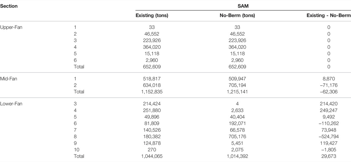
TABLE 3. Comparison of debris yield calculations for the SAM model for each section of the Fan for the berm and no-berm scenarios for the maximum event of record on 6 December 1966. The Fan hydrographic apex is the yield-limiting section of the Fan, while little attenuation in yield is expected on the mid- and lower-Fan portions.

For the sections in the FLO-2D model (Table 3), SAM predicted a total sediment yield of approximately 652,609 US tons (592,037 t) for the maximum event of record (6 December 1966) at the hydrographic apex. This is less than the sediment yield predicted by both the MUSLE equation (986,020 US tons/894,502 t) and the USACE method (1,231,303 US tons/1,117,019 t) (Table 2). By comparison, mid-Fan maximum sediment yield at Sections 1 and 2 was estimated to be 1,152,835 US tons (1,045,834 t), while lower-Fan sediment yield at Sections 3 through 10 was found to be approximately 1,044,065 US tons (947,160 t), for the same event. Interestingly, the sediment yield predictions from the MUSLE equation and the USACE method are approximately equal (MUSLE:SAM = 0.94 and USACE:SAM = 1.18) to the sediment yield predicted on the lower-Fan by the SAM model. This suggests that for the Slate Canyon alluvial fan, the MUSLE and USACE calculated sediment yield at the hydrographic apex may be used to estimate the sediment yield on the lower fan.

The ratio of apex:mid-Fan:lower-Fan yield is 1.00:1.77:1.60, suggesting there is little attenuation in the transport capacity moving down the Fan from mid- to lower-Fan, but that the Fan hydrographic apex is limiting in sediment yield. It is important to note that large volumes of deposition have not been observed at the hydrographic apex, although it is much steeper than lower down on the Fan. It may be possible, however, that the maximum event of record deposited large volumes of sediment at the hydrographic apex only to have it removed in subsequent, smaller events.

A hydraulic model of the channel above the Fan’s hydrographic apex was created to estimate the potential sediment delivery limitations based on channel geometry. The Hydraulic Engineering Center-River Analysis System model (USACE) for the peak historical event was run and the results indicate that the minimum mass capacity is approximately Qx = 2,516,000 US tons (2,282,475 t)/day at a section approximately 4,000 ft (1,219 m) upstream of the hydrographic apex. The average mass capacity is Qs = 3,992,000 US tons (3,621,481 t)/day. These capacities are larger than any of the sediment yield estimates. Specifically, the watershed yields for MUSLE and USACE are approximately Ys = 986,020 US tons (894,502 t) and 1,231,000 US tons (1,116,744 t), respectively, which is significantly less than either the minimum or average capacity of the channel. This finding indicates that the transport capacity of the channel does not limit the delivery to the Fan hydrographic apex during the peak observed event.

4 Discussion

The Keeler Dunes are situated between the toe of the Slate Canyon alluvial fan and the playa of Owens (dry) Lake. Previous studies (Lancaster and McCarley-Holder, 2013; Kolesar et al., 2022) have examined two mechanisms by which sediment may have been deposited at the dunes. In Lancaster and McCarley-Holder (2013), the authors focused on the aeolian transport of playa sediment to the Keeler Dunes. They conclude that changes to the dunes are driven by the current sediment-limited environment caused by the implementation of dust controls on the Owens Lake playa. In Kolesar et al. (2022), measurements of the potential for sediments of various desert landforms (including alluvial fans and playa surfaces) to be transported via aeolian processes demonstrate that alluvial fans can be a major source of aeolian material. In the current study, the focus is on another potential mechanism by which sediment can be deposited at a dune system; the transportation of sediment (both alluvial and aeolian in origin) via alluvial processes. This study complements previous work to creating a more complete assessment of the interconnected processes contributing to dune morphogenesis.

Sediment analysis was conducted on several areas of the Fan. The grain size distribution indicates that the Fan is made up of primarily sandy material. In general, the grain size of the fan sediments were progressively more fine with distance away from the hydrographic Fan apex, consistent with observations from other alluvial fans (Bull, 1964; Waters and Field, 1986). The sediment samples were taken in June 2013, which is at the end of the dust season (period during which the majority of aeolian sediment transportation events occur) for the Owens River Valley. At the beginning of the 2012–2013 dust season (11 October 2012), there was a large precipitation event with the capacity to transport an estimated 188,835 tons (171,308 t) to 259,503 tons (235,417 t) of sediment to the hydrographic apex (Table 2). Therefore, the samples taken had recent contributions of sediment transported via alluvial processes.

During the time between the large precipitation event and sample collection, it is also likely that material was deposited on the surface via aeolian processes. The main modes of aeolian transportation to the fan are assumed to be reptation/creep, particles > ∼0.5 mm, and saltation, particles between ∼0.07 and 0.5 mm (Kok et al., 2012). Therefore, the sediment samples with a large fraction of material with diameter ∼ 0.5 mm and smaller were likely influenced by aeolian transportation. The aeolian deposition zone is visually evident as the light color band toward the Fan toe just down-Fan from sections “lower 1” and “lower 2” (Figure 5). These influences from aeolian deposition are observed from the lower Fan area up to an elevation of approximately 3,900 ft (1,189 m), which is typical of alluvial fans in arid areas (Blair and McPherson, 2009). The contribution of fine material on the lower Fan is likely augmented by the desert pavement surfaces that trap aeolian material (McFadden et al., 1987). What is important about this observation is that aeolian deposition zones are also portions of the Fan that experience surface flows. Because the surface flows will transport material down fan toward Owens Lake and Keeler Dunes, the aeolian deposits are essentially recycled by hydraulic sediment transport processes to the lake and dunes for subsequent aeolian movement. It is presently unclear what role recycling of aeolian-derived sediments plays in the formation and maintenance of the Keeler Dunes.

The peak event of record for the Slate Canyon alluvial fan occurred on 6 December 1966. The debris production estimated by the USACE method for this date is approximately 48,500 tons/mi² (16,987,900 kg/km²). By comparison, physical measurements of the debris production of an August 1984 event in the Dolomite Fan, located north of the Slate Canyon watershed, produced 146,000 tons/mi² (51,138,834 kg/km²) (Blair and McPherson, 1998). Therefore, on a per-area basis, the Dolomite Fan produced three times the quantity of debris as the Slate Canyon Fan. However, the tributary drainage area of Dolomite Fan was approximately 1 mi² (2.6 km²) with a maximum elevation of approximately 4,000 ft (1,219 m) while the Slate Canyon watershed is approximately 25.4 mi² (64.79 km²) in size (maximum elevation near 10,000 ft [3,333 m]). Given the smaller areal extent of the Dolomite watershed, the observed higher per-area debris watershed sediment yield is expected, because the precipitation during one event could be concentrated over the entire watershed. The inverse relationship between sediment yield and drainage area was also observed in studies of the Mojave Desert of very small (1 < km²) drainage basins (Griffiths et al., 2005).

The peak event of record was used as a case study to compare between sediment transportation and surface flows during the berm and no-berm conditions. Constructed in 1954 (northern berm portion) and 1967 (southern berm portion), the diversion berms serve to protect the highway from flood inundation on the Fan up slope of State Highway 136. As illustrated in Figure 5, the construction of the berm mostly worked as intended by diverting most of the flow to two channels toward the berm extents. Similar to the natural process of channel avulsion (Leeder, 1977), this forced channel entrenchment led to changes in sedimentary deposits.

The range of watershed total debris yield is from 2,976,000 (MUSLE) to 3,943,000 (USACE) US tons (2,699,782 and 3,577,029 t, respectively) for all events greater than 1,500 cfs (42.48 m³/s) at the Fan hydrographic apex over the period of record (1948–2013, shown in Table 2). Since the SAM model results indicate that the sediment yield to the lower fan area is approximately equal to the MUSLE and USACE calculated sediment yields, this suggests a large volume of sediment has been transported down the fan via alluvial processes since 1948. Lancaster and McCarley-Holder (2013) estimated that the volume of the Keeler Dunes changed by approximately 1,150,000 US tons (1,043,262 t) (assuming the density of sand) over a similar time frame. Based on the location of the Keeler Dunes, the modeled spatial distribution of watershed deposited material, and the quantity of debris yield, it is plausible that material originating in the Slate Canyon watershed contributed to material deposited in the Keeler Dunes. Furthermore, the modeled sediment transport for the peak event of record shows that a high percentage of total sediment yield is expected to be deposited in the channels formed down-Fan of the berm edges beginning in 1954 and 1967. This change in location of sediment deposition coincides with observed migration to the southern margin of the Keeler Dunes beginning in around 1970 (Lancaster and McCarley-Holder, 2013). In arid environments such as the Owens River Valley, climatic change is often regarded as the primary cause of alluvial fan aggradation and channel abandonment and erosion (e.g., Wells et al., 1990; Bull, 1991; Harvey et al., 1999; McDonald et al., 2003). However, in the case of the Slate Canyon fan, these changes can be attributed to more direct anthropogenic forcing.

The construction of roadways and water diversion structures have a well-known impact on surface flows and sediment deposition (e.g., Jones et al., 2000; Phippen and Wohl, 2003). However, the impact of these changes on desert landforms are rarely considered. Previous studies tend to focus on the impacts of avulsion on vegetation and water, such as changes to the distribution of vegetation near the roadway (Schlesinger et al., 1989), potential contributions to desertification by increasing resource fragmentation (Okin et al., 2009), and changes to groundwater infiltration (Blainey and Pelletier, 2008). Even in the case of the Slate Canyon alluvial fan, a recent study by (Richards et al., 2022) indicates that the diversion of flow caused by berm construction is likely the driving force behind observed changes in plant cover on the alluvial fan and on the Keeler Dunes. They conclude that these changes contributed to an estimated 4.4-fold increase in sand movement compared to the theoretical scenario of no vegetation changes (Richards et al., 2022). While these are important considerations for the impacts of water diversion structures, the current study is one of the few to also implicate changes in the spatial distribution of sediment in the destabilization and morphogenesis of dunes.

5 Conclusion

The Slate Canyon watershed (25.4 mi²) is located along the eastern edge of the Owens River Valley near the town of Keeler, CA. Surface water flows discharging from the Slate Canyon provide the mechanism to convey eroding rock material from the watershed to the Fan. A diversion berm system was constructed in 1954 (northern berm portion) and 1967 (southern berm portion) on the Fan above State Highway 136. The apex of the berm system is located at approximately 3,850 ft (1,173 m). The berm system has a length of approximately 5,350 ft (1,631 m) and is comprised of two sections. The purpose of the berm system is to protect the highway from flood inundation. The Keeler Dunes are located down Fan, below State Highway 136.

In arid and semi-arid regions, the source and transportation of sediment is the subject of extensive research (e.g., Gillette et al., 1980; Reheis and Kihl, 1995; Prospero et al., 2002; Pelletier and Cook, 2005; Sweeney et al., 2011). Aeolian emissions from desiccated playas are often the focus of this research and is the preferred source in many global dust models (e.g., Tegen, 2003; Parajuli and Zender, 2017). Similarly, previous research on Keeler Dunes concluded that playa sediment transported via aeolian processes must be the source for the dunes (Lancaster and McCarley-Holder, 2013). However, based on the current use of hydrologic and hydraulic modeling to assess the potential watershed and fan sediment yield associated with Slate Canyon alluvial fan, we demonstrate that approximately 1,150,000 US tons (1,043,262 t) of sediment was moved from the alluvial fan topographic apex, down gradient toward the Keeler Dunes area from 1948 to 2013. Given the volume of sediment transported, the changes to sediment deposition caused by diversion berm construction, and the proximity of deposition to the Keeler Dunes, the Slate Canyon alluvial fan sediment is likely a major source of sediment for the dunes.

The Keeler Dunes serves as a case study into the complex alluvial-aeolian interactions that form dunes in arid environments. Dune systems around the world are subjected to anthropogenic forcing either directly through changes to sediment deposition and water channels (e.g., Ahmady-Birgani et al., 2018; Richards et al., 2022) or indirectly through climate change (e.g., Thomas et al., 2005; Bhattachan et al., 2013). As the dunes become destabilized, they can become large sources of dust, which can negatively impact downwind communities and lead to changes in nutrient distribution. This work provides an important contribution toward better understanding how alluvial fans can contribute to the genesis and cause(s) of the destabilization and migration of dune systems.

Data Availability Statement

This data can be accessed via ftp from: ftp.ncdc.noaa.gov/pub/data/noaa/.

Author Contributions

DJ and SB contributed to the conception and design of the study. DJ and SB both prepared results from portions of the models used in the study. All authors contributed to the analysis and interpretation of results. DJ, SB, and KK all wrote sections of the manuscript. All authors contributed to manuscript revision, read, and approved the submitted version.

Funding

This research and writing were supported by funds from the Los Angeles Department of Water and Power, Agreement Nos. 47557A, 47389-6, and 47169-3: Science, Technology, and Air Quality Services for Owens Lake, Owens Valley, and Mono Basin.

Author Disclaimer

The views expressed herein do not necessarily reflect the views of the funding agency.

Conflict of Interest

SB is employed by Northwest Watersheds LLC. KK is employed by Air Sciences Inc. DJ is employed by David Evans and Associates, Inc.

Publisher’s Note

All claims expressed in this article are solely those of the authors and do not necessarily represent those of their affiliated organizations, or those of the publisher, the editors and the reviewers. Any product that may be evaluated in this article, or claim that may be made by its manufacturer, is not guaranteed or endorsed by the publisher.

Acknowledgments

The authors would like to thank John Humphreys, PhD for his guidance.

Supplementary Material

The Supplementary Material for this article can be found online at: https://www.frontiersin.org/articles/10.3389/feart.2022.879115/full#supplementary-material

Footnotes

¹Uncommon abbreviations used in this article: BASINS, Better Assessment Science Integrating Point and Nonpoint Sources; CIMIS, California Irrigation Management Information System; HSPF, Hydrological Simulation Program–Fortran; MUSLE, Modified Universal Soil Loss Equation; USACE method, United States Army Corps of Engineers Los Angeles District Method; USLE, Universal Soil Loss Equation.

References

Ahmady-Birgani, H., Agahi, E., Ahmadi, S. J., and Erfanian, M. (2018). Sediment Source Fingerprinting of the Lake Urmia Sand Dunes. Sci. Rep. 8, 206. doi:10.1038/s41598-017-18027-0

PubMed Abstract | CrossRef Full Text | Google Scholar

Bacon, S. N., Jayko, A. S., Owen, L. A., Lindvall, S. C., Rhodes, E. J., Schumer, R. A., et al. (2020). A 50,000-Year Record of Lake-Level Variations and Overflow From Owens Lake, Eastern California, USA. Quat. Sci. Rev. 238, 106312. doi:10.1016/j.quascirev.2020.106312

CrossRef Full Text | Google Scholar

Beaty, C. B. (1989). Great Big Boulders I Have Known. Geology 17, 349. doi:10.1130/0091-7613(1989)017<0349:gbbihk>2.3.co;2

CrossRef Full Text | Google Scholar

Benn, D. I., Owen, L. A., Finkel, R. C., and Clemmens, S. (2006). Pleistocene Lake Outburst Floods and Fan Formation Along the Eastern Sierra Nevada, California: Implications for the Interpretation of Intermontane Lacustrine Records. Quat. Sci. Rev. 25, 2729–2748. doi:10.1016/j.quascirev.2006.02.018

CrossRef Full Text | Google Scholar

Bhattachan, A., D'Odorico, P., Okin, G. S., and Dintwe, K. (2013). Potential Dust Emissions from the Southern Kalahari's Dunelands. J. Geophys. Res. Earth Surf. 118, 307–314. doi:10.1002/jgrf.20043

CrossRef Full Text | Google Scholar

Blainey, J., and Pelletier, J. (2008). Infiltration on Alluvial Fans in Arid Environments: Influence of Fan Morphology. J. Geophys Res. 113, F03008. doi:10.1029/2007jf000792

CrossRef Full Text | Google Scholar

Blair, T. C., and McPherson, J. G. (2009). “Processes and Forms of Alluvial Fans,” in Geomorphology of Desert Environments. Editors A. J. Parsons, and A. D. Abrahams (Dordrecht: Springer Netherlands), 413–467. doi:10.1007/978-1-4020-5719-9_14

CrossRef Full Text | Google Scholar

Blair, T. C., and McPherson, J. G. (1998). Recent Debris-Flow Processes and Resultant Form and Facies of the Dolomite Alluvial Fan, Owens Valley, California. J. Sediment. Res. 68, 800–818. doi:10.2110/jsr.68.800

CrossRef Full Text | Google Scholar

Blair, T. C. (2001). Outburst Flood Sedimentation on the Proglacial Tuttle Canyon Alluvial Fan, Owens Valley, California, U.S.A. J. Sediment. Res. 71, 657–679. doi:10.1306/2dc4095e-0e47-11d7-8643000102c1865d

CrossRef Full Text | Google Scholar

Blood, W. H., and Humphrey, J. H. (1990). Design Cloudburst and Flash Flood Methodology for the Western Mojave Desert, California. ASCE, 561–566. Available at: https://cedb.asce.org/CEDBsearch/record.jsp?dockey=0067058 (Accessed April 14, 2022).

Google Scholar

Bull, W. B. (1991). Geomorphic Responses to Climatic Change. New York: Oxford University Press.

Google Scholar

Bull, W. B. (1964). Geomorphology of Segmented Alluvial Fans in Western Fresno County, California. Available at: https://pubs.er.usgs.gov/publication/pp352E (Accessed April 14, 2022). doi:10.3133/pp352e

CrossRef Full Text | Google Scholar

Cataldo, J., Behr, C., Montalto, F., and Pierce, R. (2010). Prediction of Transmission Losses in Ephemeral Streams, Western U.S.A. Open Hydrol. J. 4, 19–34. doi:10.2174/1874378101004010019

CrossRef Full Text | Google Scholar

Courant, R., Friedrichs, K., and Lewy, H. (1967). On the Partial Difference Equations of Mathematical Physics. IBM J. Res. Dev. 11, 215–234. doi:10.1147/rd.112.0215

CrossRef Full Text | Google Scholar

Danskin, W. R. (1998). Evaluation of the Hydrologic System and Selected Water-Management Alternatives in the Owens Valley, California. United States Geological Survey. doi:10.3133/wsp2370H

CrossRef Full Text | Google Scholar

D’Arcy, M., Roda-Boluda, D. C., and Whittaker, A. C. (2017). Glacial-Interglacial Climate Changes Recorded by Debris Flow Fan Deposits, Owens Valley, California. Quat. Sci. Rev. 169, 288–311. doi:10.1016/j.quascirev.2017.06.002

CrossRef Full Text | Google Scholar

Dühnforth, M., Densmore, A. L., Ivy-Ochs, S., Allen, P. A., and Kubik, P. W. (2007). Timing and Patterns of Debris-Flow Deposition on Shepherd and Symmes Creek Fans, Owens Valley, California, Deduced from Cosmogenic 10Be. J. Geophys Res. Earth Surf. 112, F03S15. doi:10.1029/2006JF000562

CrossRef Full Text | Google Scholar

FLO-2D Software Inc. (2021). FLO-2D Tutorials. Available at: https://documentation.flo-2d.com/ (Accessed May 12, 2022).

Google Scholar

Gatwood, E., Pedersen, J., and Casey, K. (2000). Los Angeles District Debris Method for Prediction of Debris Yield. Los Angeles, CA: United States Army Corps of Engineers. Available at: https://www.scribd.com/document/474221265/US-Army-Corps-of-Engineers-Los-Angeles-District-Debris-Method (Accessed April 14, 2022).

Google Scholar

Gillette, D. A., Adams, J., Endo, A., Smith, D., and Kihl, R. (1980). Threshold Velocities for Input of Soil Particles into the Air by Desert Soils. J. Geophys. Res. 85, 5621–5630. doi:10.1029/jc085ic10p05621

CrossRef Full Text | Google Scholar

Griffiths, P. G., Hereford, R., and Webb, R. H. (2005). Sediment Yield and Runoff Frequency of Small Drainage Basins in the Mojave Desert, United States. Geomorphology 74, 232–244. doi:10.1016/j.geomorph.2005.07.017

CrossRef Full Text | Google Scholar

Harvey, A. M., Wigand, P. E., and Wells, S. G. (1999). Response of Alluvial Fan Systems to the Late Pleistocene to Holocene Climatic Transition: Contrasts Between the Margins of Pluvial Lakes Lahontan and Mojave, Nevada and California, USA. Catena 36, 255–281. doi:10.1016/s0341-8162(99)00049-1

CrossRef Full Text | Google Scholar

Homer, C. G., Dewitz, J., Fry, J., Coan, M., Hossain, N., Larson, C., et al. (2007). Completion of the 2001 National Land Cover Database for the Conterminous United States. Photogramm. Eng. Remote Sens. 73, 5. Available at: http://pubs.er.usgs.gov/publication/70029996 (Accessed April 15, 2022).

Google Scholar

Hubert, J. F., and Filipov, A. J. (1989). Debris-Flow Deposits in Alluvial Fans on the West Flank of the White Mountains, Owens Valley, California, U.S.A. Sediment. Geol. 61, 177–205. doi:10.1016/0037-0738(89)90057-2

CrossRef Full Text | Google Scholar

Jackson, W. L., Gebhardt, K., and Van Haveren, B. P. (1986). “Use of the Modified Universal Soil Loss Equation for Average Annual Sediment Yield Estimates on Small Rangeland Drainage Basins,” in IAHS-AISH Publication (Wallingford: International Association of Hydrological Sciences), 413–423. Available at: http://pascal-francis.inist.fr/vibad/index.php?action=getRecordDetail&idt=8269889 (Accessed March 31, 2022).

Google Scholar

Jaffe, D. A. (2008). Examination of an Arithmetic Approach for the Coupling of Two-Dimensional Hydraulic Surface Water Models. FMA News (December) 18 (4), 13–18.

Google Scholar

Jones, J. A., Swanson, F. J., Wemple, B. C., and Snyder, K. U. (2000). Effects of Roads on Hydrology, Geomorphology, and Disturbance Patches in Stream Networks. Conserv. Biol. 14, 76–85. Available at: https://www.jstor.org/stable/2641906 (Accessed April 14, 2022). doi:10.1046/j.1523-1739.2000.99083.x

CrossRef Full Text | Google Scholar

Kok, J. F., Parteli, E. J., Michaels, T. I., and Karam, D. B. (2012). The Physics of Wind-Blown Sand and Dust. Rep. Prog. Phys. 75, 106901. doi:10.1088/0034-4885/75/10/106901

PubMed Abstract | CrossRef Full Text | Google Scholar

Kolesar, K. R., Schaaf, M. D., Bannister, J. W., Schreuder, M. D., and Heilmann, M. H. (2022). Characterization of Potential Fugitive Dust Emissions Within the Keeler Dunes, an Inland Dune Field in the Owens Valley, California, United States. Aeolian Res. 54, 100765. doi:10.1016/j.aeolia.2021.100765

CrossRef Full Text | Google Scholar

LaMotte, A. E. (2016). National Land Cover Database 2001 (NLCD01). Reston VA: U.S. Geological Survey. doi:10.3133/ds383

CrossRef Full Text | Google Scholar

Lancaster, N., Baker, S., Bacon, S., and McCarley-Holder, G. (2015). Owens Lake Dune Fields: Composition, Sources of Sand, and Transport Pathways. CATENA 134, 41–49. doi:10.1016/j.catena.2015.01.003

CrossRef Full Text | Google Scholar

Lancaster, N., and McCarley-Holder, G. (2013). Decadal-Scale Evolution of a Small Dune Field: Keeler Dunes, California 1944-2010. Geomorphology 180-181, 281–291. doi:10.1016/j.geomorph.2012.10.017

CrossRef Full Text | Google Scholar

Langbein, W. B., and Schumm, S. A. (1958). Yield of Sediment in Relation to Mean Annual Precipitation. Trans. AGU 39, 1076–1084. doi:10.1029/tr039i006p01076

CrossRef Full Text | Google Scholar

Leeder, M. R. (1977). A Quantitative Stratigraphic Model for Alluvium, with Special Reference to Channel Deposit Density and Interconnectedness. Fluv. Sedimentol. 5, 587–596. Available at: https://archives.datapages.com/data/dgs/005/005001/587_cspgsp0050587.htm (Accessed April 14, 2022).

Google Scholar

McDonald, E., McFadden, L., and Wells, S. (2003). “Regional Response of Alluvial Fans to the Pleistocene-Holocene Climatic Transition, Mojave Desert, California,” in Paleoenvironments and Paleohydrology of the Mojave and Southern Great Basin Deserts (Boulder, CO: Geological Society of America), 189–205. doi:10.1130/0-8137-2368-x.189

CrossRef Full Text | Google Scholar

McFadden, L. D., Wells, S. G., and Jercinovich, M. J. (1987). Influences of Eolian and Pedogenic Processes on the Origin and Evolution of Desert Pavements. Geology 15, 504–508. doi:10.1130/0091-7613(1987)15<504:ioeapp>2.0.co;2

CrossRef Full Text | Google Scholar

Miller, D. M., Schmidt, K. M., Mahan, S. A., McGeehin, J. P., Owen, L. A., Barron, J. A., et al. (2010). Holocene Landscape Response to Seasonality of Storms in the Mojave Desert. Quat. Int. 215, 45–61. doi:10.1016/j.quaint.2009.10.001

CrossRef Full Text | Google Scholar

Muhs, D. R., Lancaster, N., and Skipp, G. L. (2017). A Complex Origin for the Kelso Dunes, Mojave National Preserve, California, USA: A Case Study Using a Simple Geochemical Method with Global Applications. Geomorphology 276, 222–243. doi:10.1016/j.geomorph.2016.10.002

CrossRef Full Text | Google Scholar

Mussetter, R. A., Lagasse, P. F., and Harvey, M. D. (1994). Sediment and Erosion Design Guide. Prepared for Albuquerque Metropolitan Arroyo Flood Control Authority AMAFCA.

Google Scholar

Okin, G. S., Parsons, A. J., Wainwright, J., Herrick, J. E., Bestelmeyer, B. T., Peters, D. C., et al. (2009). Do Changes in Connectivity Explain Desertification? BioScience 59, 237–244. doi:10.1525/bio.2009.59.3.8

CrossRef Full Text | Google Scholar

Osborn, G., and Bevis, K. (2001). Glaciation in the Great Basin of the Western United States. Quat. Sci. Rev. 20, 1377–1410. doi:10.1016/s0277-3791(01)00002-6

CrossRef Full Text | Google Scholar

Parajuli, S. P., and Zender, C. S. (2017). Connecting Geomorphology to Dust Emission Through High-Resolution Mapping of Global Land Cover and Sediment Supply. Aeolian Res. 27, 47–65. doi:10.1016/j.aeolia.2017.06.002

CrossRef Full Text | Google Scholar

Pelletier, J. D., and Cook, J. P. (2005). Deposition of Playa Windblown Dust Over Geologic Time Scales. Geology 33, 909–912. doi:10.1130/g22013.1

CrossRef Full Text | Google Scholar

Phippen, S. J., and Wohl, E. (2003). An Assessment of Land Use and Other Factors Affecting Sediment Loads in the Rio Puerco Watershed, New Mexico. Geomorphology 52, 269–287. doi:10.1016/s0169-555x(02)00261-1

CrossRef Full Text | Google Scholar

Prospero, J. M., Ginoux, P., Torres, O., Nicholson, S. E., and Gill, T. E. (2002). Environmental Characterization of Global Sources of Atmospheric Soil Dust Identified with the Nimbus 7 Total Ozone Mapping Spectrometer (Toms) Absorbing Aerosol Product. Rev. Geophys. 40, 2-1–2–31. doi:10.1029/2000rg000095

CrossRef Full Text | Google Scholar

Reheis, M. C., and Kihl, R. (1995). Dust Deposition in Southern Nevada and California, 1984-1989: Relations to Climate, Source Area, and Source Lithology. J. Geophys. Res. 100, 8893–8918. doi:10.1029/94jd03245

CrossRef Full Text | Google Scholar

Richards, J. H., Smesrud, J. K., Williams, D. L., Schmid, B. M., Dickey, J. B., and Schreuder, M. D. (2022). Vegetation, Hydrology, and Sand Movement Interactions on the Slate Canyon Alluvial Fan-Keeler Dunes Complex, Owens Valley, California. Aeolian Res. 54, 100773. doi:10.1016/j.aeolia.2022.100773

CrossRef Full Text | Google Scholar

Schlesinger, W. H., Fonteyn, P. J., and Reiners, W. A. (1989). Effects of Overland Flow on Plant Water Relations, Erosion, and Soil Water Percolation on a Mojave Desert Landscape. Soil Sci. Soc. Am. J. 53, 1567–1572. doi:10.2136/sssaj1989.03615995005300050045x

CrossRef Full Text | Google Scholar

Schumm, S. A. (1977). The Fluvial System. Chichester and New York: John Wiley & Sons. Available at: https://onlinelibrary.wiley.com/doi/abs/10.1002/esp.3290040121 (Accessed March 15, 2022).

Google Scholar

Simons, D. B., and Sentürk, F. (1992). Sediment Transport Technology: Water and Sediment Dynamics. Littleton, CO: Water Resources Publications.

Google Scholar

Soil Survey StaffNational Resources Conservation Service (2022). United States Department of Agriculture Web Soil Survey. Available at: https://websoilsurvey.sc.egov.usda.gov/App/WebSoilSurvey.aspx (Accessed March 15, 2022).

Google Scholar

Sweeney, M. R., McDonald, E. V., and Etyemezian, V. (2011). Quantifying Dust Emissions From Desert Landforms, Eastern Mojave Desert, USA. Geomorphology 135, 21–34. doi:10.1016/j.geomorph.2011.07.022

CrossRef Full Text | Google Scholar

Sweeney, M. R., McDonald, E. V., and Markley, C. E. (2013). Alluvial Sediment or Playas: What Is the Dominant Source of Sand and Silt in Desert Soil Vesicular A Horizons, Southwest USA. J. Geophys. Res. Earth Surf. 118, 257–275. doi:10.1002/jgrf.20030

CrossRef Full Text | Google Scholar

Tatum, F. E. (1963). A New Method of Estimating Debris-Storage Requirements for Debris Basins. Los Angeles, CA: U.S. Army Engineer District.

Google Scholar

Tegen, I. (2003). Modeling the Mineral Dust Aerosol Cycle in the Climate System. Quat. Sci. Rev. 22, 1821–1834. doi:10.1016/s0277-3791(03)00163-x

CrossRef Full Text | Google Scholar

Thomas, D. S. G., Knight, M., and Wiggs, G. F. S. (2005). Remobilization of Southern African Desert Dune Systems by Twenty-First Century Global Warming. Nature 435, 1218–1221. doi:10.1038/nature03717

PubMed Abstract | CrossRef Full Text | Google Scholar

Thomas, W. A., Copeland, R. R., and McComas, D. N. (2002). SAM Hydraulic Design Package for Channels. Vicksburg, MS: U.S. Army Corps of Engineers Engineer Research and Development Center. Available at: https://dokumen.tips/reader/f/sam-hydraulic-design-package-for-channels-sam-hydraulic-design-package-for-channels.

Google Scholar

United States Department of the Interior Geological Survey (USDIGS) (1982). Guidelines for Determining Flood Flow Frequency, 17B [Since Superseded by 17C]. Reston VA: US Department of the Interior Geological Survey Office of Water Data Coordination. Available at: https://water.usgs.gov/osw/bulletin17b/dl_flow.pdf (Accessed April 27, 2022).

Google Scholar

United States Environmental Protection Agency (USEPA) (2019). BASINS 4.5 (Better Assessment Science Integrating Point & Non-Point Sources) Modeling Framework. BASINS Core Manual. Available at: https://www.epa.gov/sites/production/files/2019-03/documents/basins4.5coremanual.2019.03.pdf (Accessed March 31, 2022).

Google Scholar

von Holdt, J., Eckardt, F. D., Baddock, M. C., and Wiggs, G. F. S. (2019). Assessing Landscape Dust Emission Potential Using Combined Ground-Based Measurements and Remote Sensing Data. J. Geophys. Res. Earth Surf. 124, 1080–1098. doi:10.1029/2018JF004713

CrossRef Full Text | Google Scholar

Waananen, A. O., and Crippen, J. R. (1977). Magnitude and Frequency of Floods in California. Water Resources Division, U.S. Geological Survey. Available Through the National Technical Information Service. doi:10.3133/wri7721

CrossRef Full Text | Google Scholar

Waters, M. R., and Field, J. J. (1986). Geomorphic Analysis of Hohokam Settlement Patterns on Alluvial Fans Along the Western Flank of the Tortolita Mountains, Arizona. Geoarchaeology 1, 329–345. doi:10.1002/gea.3340010401

CrossRef Full Text | Google Scholar

Wells, S. G., McFadden, L. D., and Harden, J. (1990). “Preliminary Results of Age Estimations and Regional Correlations of Quaternary Alluvial Fans within the Mojave Desert of Southern California,” in At the End of the Mojave: Quaternary Studies in the Eastern Mojave Desert: San Bernardino County Museum Association and 1990 Mojave Desert Quaternary Research Center Symposium. Editors R. E. Reynolds, S. G. Wells, R. H. Brady, and J. Reynolds (Redlands, CA: San Bernadino County Museum Association), 45–53.

Google Scholar

Yang, C. T., and Huang, C. (2001). Applicability of Sediment Transport Formulas. Int. J. Sediment. Res. 16, 335–353. Available at: https://www.researchgate.net/publication/282266374_Applicability_of_sediment_transport_formulas.

Google Scholar

Zhong, S., Li, J., Whiteman, C. D., Bian, X., and Yao, W. (2008). Climatology of High Wind Events in the Owens Valley, California. Mon. Weather Rev. 136, 3536–3552. doi:10.1175/2008mwr2348.1

CrossRef Full Text | Google Scholar