 Simone Schauwecker
 Gabriel Palma
 Shelley MacDonell
 Álvaro Ayala
 Maximiliano Viale
- 1Centro de Estudios Avanzados en Zonas Áridas (CEAZA), La Serena, Chile
- 2Waterways Centre for Freshwater Management, University of Canterbury and Lincoln University, Christchurch, New Zealand
- 3Instituto Argentino de Nivología, Glaciología y Ciencias Ambientales (IANIGLA-CONICET), Mendoza, Argentina
Understanding the variability of the snowline and the closely related 0°C isotherm during infrequent precipitation events in the dry Andes in Chile is fundamental for precipitation, snow cover, and discharge predictions. For instance, it is known that on the windward side of mountains, the 0°C isotherm can be several hundreds of meters lower than on the free air upwind counterpart, but little is understood about such effects in the Andes due to missing in situ evidence on the precipitation phase. To bridge this gap, 111 photographs of the snowline after precipitation events between 2011 and 2021 were gathered in the frame of a citizen science programme to estimate the snowline altitude. Since photographs of the mountain snowline are in good agreement with Sentinel-2 imagery, they have great potential to validate empirical snowline estimations. Using the snowline altitude from the photos, we evaluated different methods to estimate the snowline and 0°C isotherm altitude during precipitation events based on surface meteorological observations and ERA5 reanalysis data. We found a high correlation between the observed snowline altitude and the extrapolated 0°C isotherm based on constant lapse rates (−5.5 to −6.5°C km−1) applied to air temperature from single, near stations. However, uncertainty increases for distances >10 km. The results also indicate that the linear regression method is a good option to estimate ZSL, but the results strongly depend on the availability of high-elevation station datasets. During half of the precipitation events, the 0°C isotherm lies between ∼1,800 and ∼2,400–2,500 m asl. in winter, and the snowline is on average ∼280 m below this altitude. Our results indicate the presence of a mesoscale lowering of the 0°C isotherm over the windward slopes compared to the free-air upwind value during precipitation events and a possible isothermal layer of near-freezing air temperatures comparable to other mountain ranges. Due to this mesoscale and local behavior, ERA5 data generally overestimate the snow–rain transition in high-elevation areas, especially for relatively intense events. On the other hand, the 0°C isotherm altitude is underestimated if only low-elevation valley stations are considered, highlighting the importance of high-altitude meteorological stations in the network.
1 Introduction
Over the semi-arid Andes of Chile, most frontal storms occur in winter and usually leave snow at high elevations. After such precipitation events, a clear horizontal snowline (ZSL) divides the snow-covered mountain tops from the lower, snow-free areas, and valley floors. The altitude of the snowline is closely linked to the altitude of the 0°C isotherm (Z0C) and defines the pluvial area of mountainous catchments. A difference of a few hundred meters between a cold and a warm event can, therefore, induce a significant difference in the pluvial area with quite distinct consequences for discharge and floods (Ibañez et al., 2020; White et al., 2002). During the last four decades, the snow–rain transition altitude has increased over global land surfaces (Prein and Heymsfield, 2020), and a further upward shift is expected in the future, altering snow pack dynamics and streamflow timing and amount (Mardones and Garreaud, 2020; Jara et al., 2021). Appropriate methods to estimate the event-to-event variability and spatial patterns of the snow–rain transition over mountainous regions are, therefore, crucial for the assessment of precipitation triggered natural hazards (Vergara Dal Pont et al., 2018), hydrological modeling, and monitoring of snow cover (Harpold et al., 2017), glaciers, and runoff (Immerzeel et al., 2014; Schauwecker et al., 2017; Lute and Abatzoglou, 2020) and also for meteorological forecasts needed for the navigability of roadways, tourism, or agriculture (White et al., 2010; Thériault et al., 2012; Sumargo et al., 2020).
The terms snowline (ZSL), 0°C isotherm (Z0C), and snow–rain transition have distinct definitions and sometimes there is confusion between them. The snowline (ZSL) is usually defined as the actual lower limit of the snow cover on the ground (AMS, 2021). Whether snow accumulates on the ground or instantaneously melts depends on the conditions of the soil such as surface temperature and vegetation type. Z0C is usually defined as the lowermost altitude in the atmosphere with 0°C and corresponds approximately to the altitude where ice crystals and snowflakes begin to melt as they descend through the atmosphere (AMS, 2021). In most meteorological weather forecasts, the altitude of Z0C is used to refer to the snow–rain transition, but this term is ambiguous because, in reality, the snow does not transform instantaneously into rain (Minder and Kingsmill, 2013). The transition occurs within an atmospheric altitude interval of several hundred meters, the so-called snow–rain transition zone (or melting layer, Figure 1). During precipitation, Z0C lies at the top of the snow–rain transition zone in which both frozen and liquid hydrometeors coexist (AMS, 2021). Below the Z0C altitude, an isothermal layer of nearly 0°C may form (Findeisen, 1940; Marwitz, 1983; Unterstrasser and Zängl, 2006; Thériault et al., 2015). In general, an isothermal layer is defined as a vertical column of air having a constant temperature with height. Such an isothermal layer of near 0°C or slightly warmer occurs, for example, during intense stratiform precipitation or over mountainous regions if the initial Z0C is sufficiently far below the crest height of the surrounding mountain ridges so that the air mass in the valley becomes decoupled from the environmental flow aloft. If this happens, latent heat for melting falling snow is removed from the valley air until the snowline reaches the valley bottom, forming thick air layers at near 0°C. This diabatic cooling effect is enhanced with high precipitation intensities (Thériault et al., 2012) and this zone can reach up to 1 km deep (Marwitz, 1983), depending on the complex interplay between air humidity and temperature profiles and hydrometeor size, density, type, and fall velocity (Matsuo and Sasyo, 1981). Despite its importance, the formation of an isothermal layer is not considered in most air temperature extrapolation approaches.
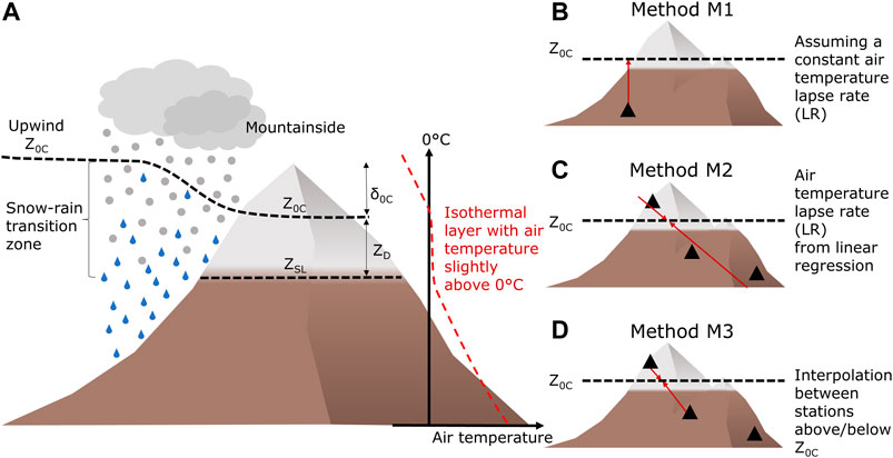
FIGURE 1. (A) Scheme showing the terminology used in this work (adapted from Minder et al., 2011). Black dashed lines show the altitude of the 0°C isotherm (Z0C) and the snowline (ZSL). The difference between the mountainside Z0C and ZSL is named ZD, and δ0C is the displacement between the mountainside Z0C and its upwind value (also called “lowering”). The red dashed line shows a typical vertical air temperature profile when an isothermal layer forms; Schematic diagrams illustrating the three methods used: (B) M1, (C) M2, and (D) M3.
In addition to the isothermal layer, there are other mechanisms that need to be considered to study the mesoscale variability of the snowline. Even though the mountainside Z0C is closely tied to the free troposphere Z0C during precipitation events, Z0C over windward slopes of mountains can be several hundred meters below the free atmosphere counterpart, as illustrated in Figure 1 (Medina et al., 2005; Minder et al., 2011; Cui et al., 2020). This offset—called mesoscale lowering of Z0C—has been found to be, for example, on average, 170 m for the Sierra Nevada (Minder and Kingsmill, 2013). Due to this mesoscale phenomenon, the Z0C measured by radiosonde data on the coast might be higher than its counterpart over the mountains in Chile when it is raining, leading to uncertainties in hydrological modeling. For instance, Minder et al. (2011) named three main mechanisms for the mesoscale lowering of Z0C over mountains: 1) Orographically enhanced hydrometeors population over the mountain slopes leads to more latent cooling of the air by the melting of precipitation; 2) the melting distance of the hydrometeors in the snow–rain transition zone might increase over mountains; and 3) adiabatic cooling and expansion of air parcels that are forced to rise over a topographic barrier. Here, we do not focus on the role of the different mechanisms causing a mesoscale drop of Z0C, but rather, we examine whether there is a lowering with potential implications for mountain hydroclimate.
Even if the decrease of Z0C of several hundred meters might have important implications for snow accumulation and runoff, it has only been observed in model simulations by Viale et al. (2013), but has not been studied in-depth or quantified so far for the Chilean Andes. The main challenge of studying this effect is in acquiring ground-based precipitation phase observations. In Continental Chile, there are only four radiosonde sites (Antofagasta, Santo Domingo, Puerto Montt, and Punta Arenas, Figure 2A), which are all located at the coast and no ground radar observations are available as in other mountainous regions (Fabry and Zawadzki, 1995; White et al., 2002; Lundquist et al., 2008). Also, most weather stations are located in the lowlands or in valley bottoms, influenced by either maritime or continental mountainous near-surface conditions and so the assumption of free-atmosphere temperature lapse rates may not be valid. In addition, generally, satellite images are only able to provide snow cover a few days after the event (due to cloud cover or visiting frequency) when most snow has already disappeared—especially on north-facing slopes (Lagos-Zúñiga and Vargas-Mesa, 2014).
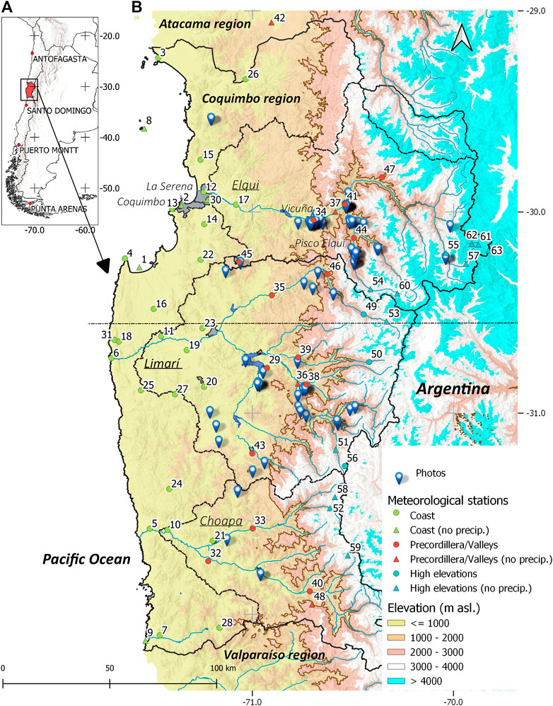
FIGURE 2. (A) Location of the study region (Coquimbo Region, Chile) and radiosonde launch sites in Chile. (B) Map of the study region with the location of photographic evidence from the participatory science programme and meteorological stations. The 2,000 m asl. isoline is indicated with a brown line. The station numbers follow their elevational distribution from 1 (lowest) to 63 (highest). (Source: catchment outlines are from the CAMELS-CL dataset, Alvarez-Garreton et al., 2018, hydrological information is provided by the Chilean government, and topographic information comes from SRTM DEM. Topographic information and country outlines in the small map are provided by NASA EarthData).
To fill the gap of missing measurements, this work is based on a set of photos of the mountainside snowline shortly after precipitation events. A photograph reveals in situ information about the snowline altitude and can be used to assess different methods to estimate the snow–rain transition. Furthermore, a photo can deliver information on cloudy days when passive satellite sensors are not able to capture surface conditions. The photograph collection used in this work is the result of a citizen science programme promoted by the Centro de Estudios Avanzados en Zonas Áridas (CEAZA). CEAZA is a regional research center located in the Coquimbo Region. Part of its mission is the promotion of the participation of the local community in science. This initiative has served to get the local society involved in science and to add value to science in society. Recently, snow cover monitoring using webcam images (Portenier et al., 2020), time-lapse cameras (Liu et al., 2015), or direct visual observations of the precipitation type (Knowles et al., 2006; Froidurot et al., 2014) have been used, but to our knowledge, the potential of photographs or any other direct visual inspection for validating extrapolation methods has not been published for the Andes.
The objectives of this work are as follows: 1) quantify Z0C and ZSL during precipitation events in the Coquimbo Region (Figure 2B) with different methods and based on photographs, station data, and climate reanalysis; 2) present the strengths and limitations of the different methods; and 3) evaluate the possible existence of the mesoscale lowering of Z0C over the windward slope of the Andes and the appearance of isothermal layers.
2 Geographical Setting
The semi-arid Coquimbo Region of Chile (∼29–32°S) is located in the transitional zone between the hyper-arid Atacama Desert to the north and the temperate sector of Central Chile to the south. The region is bounded to the west by the Pacific Ocean and to the east by the high main divide of the Andes mountain range (>5,000 m), with its highest elevations only at a distance of about 150 km from the coast (Figure 2B). In the Coquimbo Region, there are three main large watersheds (from north to south: Elqui, Limarí, and Choapa), with extensive agricultural activities that highly depend on meltwater from the mountain cryosphere, mostly from the winter snow cover above approximately 2,000 m asl., as indicated on the map.
The mean annual precipitation in low-lying regions is ∼50 mm in the Elqui River basin in the north of the Coquimbo Region and ∼300 mm for the Choapa River catchment in the south (Favier et al., 2009; Alvarez-Garreton et al., 2018). Due to the north–south gradient in both air temperature and precipitation, we divided our studied region into two clusters named sub-regions Elqui (29.0–30.55°S) and Limarí/Choapa (30.55–32.0°S, Figure 2B), following the suggestions by Lute and Abatzoglou (2020). There is also a strong orographic precipitation enhancement, leading to over 300 mm of annual precipitation in the upper Elqui river basin (>3,000 m asl.), while annual precipitation is less than 100 mm at the coast (Falvey and Garreaud, 2009; Favier et al., 2009; Scaff et al., 2017). Over 90% of the total annual precipitation occurs during the austral winter (April–September), and a large part of the annual precipitation falls during two to three events per year, which contribute 60% of the total precipitation at the coast and 40% at the highlands (Scaff et al., 2017). Heavy events and snow accumulation are strongly related to intense water vapor transport from the Pacific Ocean in the pre-cold–front environment of extratropical cyclones, which have been named as atmospheric rivers (Viale and Nuñez, 2011; Viale et al., 2018; Saavedra et al., 2020). Since annual precipitation depends on a few winter storms, there is an extremely large interannual variability, largely modulated by the ENSO phenomenon (Rutllant and Fuenzalida, 1991). The last decade was especially dry in Central Chile (30–38°S), with most years showing below-normal annual precipitation, the so-called central Chile megadrought (Garreaud et al., 2017, 2020).
3 Data and Methodology
In this work, we focus on the estimation of Z0C and ZSL during precipitation events. A precipitation day is often defined where a meteorological station records precipitation exceeding some threshold (1 mm day−1, Ibañez et al., 2020 or 5 mm day−1, Mardones and Garreaud, 2020). But the definition of a regionally significant precipitation event is not straightforward since precipitation can be local, of low intensity, or limited to the highest elevations where stations are scarce or do not record precipitation. Therefore, we here defined a precipitation day where at least three stations in the region recorded ≥2 mm. By using this criterion, days with marine drizzle producing only traces of rain on the coast are excluded. To apply this criterion, we used all stations within the Coquimbo Region (see Figure 2B) with hourly precipitation records. Daily precipitation is computed starting from 00 local time (04 UTC). If precipitation days are separated by 1 day or more the event was split.
3.1 Methods for the Estimation of Z0C and ZSL
3.1.1 ZSL Derived From Photographs of Citizen Science Programme
To assess different methods that estimate Z0C or ZSL, we used photos collected in the frame of the citizen science programme “Vecinos de las Nieves” (CEAZA, 2021). In April 2021, we requested photos of past and current precipitation events via social networks (Figure 3A), asking for the following information: location, name of the mountain, direction of the camera, date, and hour. By sending the photo, the participants agreed that the photo could be used for scientific purposes. Nearly 70 participants sent photos taken since 2011. In addition, we gathered photos from social networks (Facebook, Twitter, and Flickr). In total, 111 photographs were selected from 28 events over 11 years (2011–2021). All the photos (Supplementary Figure S6) and the details (Supplementary Table S2) can be found in the supplementary information. We selected the photos that fulfilled the following criteria:
- Date, hour, and location of the photo are available and can be verified.
- A clear snowline is visible and the resolution of the photo allows identifying its altitude.
- The photo was captured less than 48 h after the end of precipitation according to the closest meteorological records. Most photos were taken <12 h after precipitation ended, but it must be noted that snow might melt or sublimate within a few hours.
- If there are several photos from the same site, we only selected the first one that was taken after the precipitation stopped.
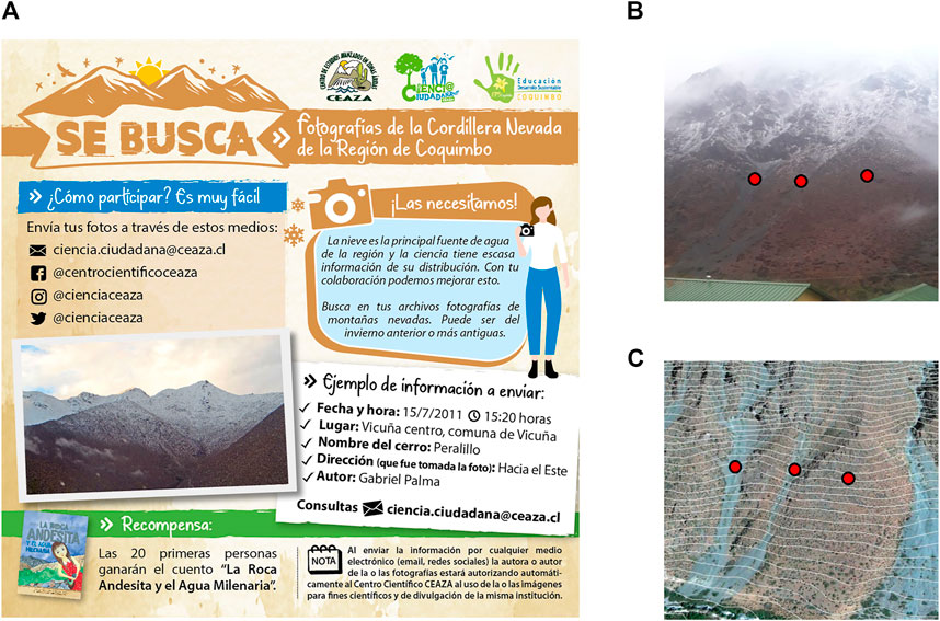
FIGURE 3. (A) Social media flyer used to collect photos of the snowline. An example of (B) a photo of the snowline (M. Carmona 23 June 2021) and (C) isolines generated based on a DEM and visualized in Google Earth. The red points mark the visually identified snowline. The photo indicates ZSL of ∼1,561 m asl.
The aim of the photograph analysis is to derive a representative value of ZSL per photo. To do so, three representative points on the mountain slope were drawn on the photo at the lowermost elevation with snow occurrence (Figure 3B). The photo was then compared to isolines in the Google Earth software to estimate the elevation of the selected points using geological features as reference (Figure 3C). The mean altitude of the three points was then calculated. Topographic isolines have a vertical distance of 12.5 m and were computed based on the Advanced Land Observation Satellite (ALOS) Digital Elevation Model (DEM) (PALSAR 2011, from Japan Aerospace Exploration Agency, JAXA, 2011).
This method might be inappropriate in cases where new snow lies above the lower extent of the current snow cover. However, this did not occur in any of the photos. We expect that such events are infrequent in this arid region, mainly because precipitation events are often separated by several days or weeks and because snow melts/sublimates quickly at low altitudes (Réveillet et al., 2020).
In the presented methodology, we compared the snowline altitude from the photos to the minimum Z0C during an event. The photos from two precipitation events of 8–10 August 2015 and 10–12 May 2017, both of which caused floods and mass movements in Vicuña and its surroundings (Palma, 2019), were not considered in the following analyses because air temperature significantly increased during the last hours of the event, probably causing rain on snow and leaving a significantly higher ZSL compared to the minimum Z0C during the event (Supplementary Figure S4 in the supplementary information). It seems thus that for events with increasing air temperatures during the last hours, the minimum Z0C is not a good estimator for the final ZSL after the event. For such events, the Z0C during the last relevant precipitation hours would be a better estimate. Other precipitation events with increasing air temperatures have been observed during the study period, but the increase only occurred during the final hours of the events and was accompanied by low precipitation intensities.
In addition, we excluded the photo from the event on 23–24 June 2020, where the snowline from the photo clearly lay almost 600 m above the minimum Z0C from nearby stations. The closest station, station 46 at a distance of 9 km, showed a clear drop in air temperature, which probably did not occur at the photo site. For example, the nearby station 49 did not show this drop in air temperature. This case shows that a temperature drop at an individual station can lead to errors in the method.
3.1.2 ZSL Derived From Satellite Images
We used the snow cover area maps derived from Sentinel-2 images at a spatial resolution of ca. 55 m. The maps are automatically derived by the Sentinel-2 Level 2A processing using the Normalized Difference Snow Index (NDSI) (European Space Agency, 2022). To estimate ZSL, we used the approach presented by Gascoin et al. (2019). We considered the area of the Elqui River basin, fitting a rectangle to the catchment area. We then selected all available snow cover area maps <5 days after precipitation events 2016–2021, resulting in ten images. A DEM from the Shuttle Radar Topography Mission (SRTM) was used to segment the satellite image in elevation bands with a fixed height of 100 m. Then, the fraction of the area covered by snow in each band was computed. The simple algorithm proposed by Gascoin et al. (2019) finds the lowest elevation band at which the snow cover fraction is greater than a given fraction fs selected as 2%. The value of ZSL is then the lower edge of that elevation band. It should be noted that Gascoin et al. (2019) selected the fraction fs of 10% and then defined the snowline in two elevation bands below that band. Here, we found that our criteria lead to a slightly higher correlation between the snowline altitude from satellites and photos. In total, we could verify the ZSL of 22 photos during 10 events.
3.1.3 Z0C Derived From Ground Stations
The Coquimbo Region contains a dense network of automatic meteorological stations maintained by the CEAZA research institute (Supplementary Table S1). Air temperature, precipitation and other variables are recorded at 10 min intervals and then averaged to hourly data. Most stations were installed between 2004 and 2010, and their elevations range between sea level and 4,774 m asl. Precipitation and air temperature data were used to estimate Z0C through three different traditional methods and for the period 2011–2021.
The first method (M1, Figure 1B) is based on data from a single meteorological station and the assumption that temperature decreases with altitude following a certain constant lapse rate (Eq. 1). We evaluate different typical free air temperature lapse rates under moisture saturated conditions, ranging from −5 to −6.5°C km−1 (Blandford et al., 2008; Minder et al., 2010; Garreaud, 2013; González and Garreaud, 2019; Ibañez et al., 2020; Mardones and Garreaud, 2020). In addition, in hydrological models, a threshold temperature TSL of around 1–2°C is usually used to discriminate between snow and rain at certain elevation bands (Schaefli et al., 2005, Eq. 2). This threshold temperature corresponds to the air temperature at which snowflakes can reach the ground below Z0C without melting (at the snowline) and therefore, in theory, relates to the offset ZD between Z0C and ZSL, see Figure 1. The air temperature at the altitude of the snowline is, however, substantially uncertain and depends on a variety of variables such as humidity, precipitation rate, soil temperature or vegetation type. The equations are as follows:
and
where Z0C is the altitude of the 0°C isotherm, ZSL is the snowline altitude, ZSt and TSt are station elevation and air temperature, TSL is the threshold air temperature at the snowline altitude, and LR is the air temperature lapse rate.
In detail, the following steps were performed to compare Z0C from Eq. 1 to ZSL from photos taken within a certain time after precipitation end (T1): For every station within a certain distance (Dst) to the photo, Z0C was estimated with Eq. 1 and different LRs (−5, −5.5, −6, and −6.5°C km−1) for all rainy hours (≥0.2 mm h−1) within a defined time window before the photo capture (T2). From the rainy hours, we then selected the hour with the lowest Z0C, assuming that this value is most decisive for the final snowline observed in the photo. For each photo and LR, we derived n values of Z0C depending on the number of stations within the searching distance. For each LR, the mean Z0C of the n values was compared to the ZSL for all photos. From all these data pairs per LR, mean offset, standard deviation (SD), and coefficient of determination (R2) were computed. The highest R2 values indicate the most suitable LRs, and the coefficient of determination is an indicator of the uncertainty. The mean offset corresponds in part to the difference ZD between Z0C and ZSL, even though it might also be influenced by local conditions at the station or nearby the snowline and needs careful evaluation. Nevertheless, this offset was used to estimate TSL (TSL = ZD‧LR), which is required for Eq. 2. This equation was then applied to stations within 50 km with the aim to better understand the behavior and representativeness of different stations to estimate ZSL with M1 in the function of distance and elevation (Section 4.2.2).
The following decisions were made for the method M1: 1) DSt: Stations within a 10 km distance to the photo location were selected. If the distance is shorter, a considerable number of photos is not close enough to stations and needs to be excluded. If the distance is larger, the representativity of the stations decreases. 2) T1: We included only photos taken ≤12 h after precipitation end. Some of the selected photos were taken up to 24 h after precipitation end and showed, in some cases, a relatively high snowline compared to Z0C since snow might have melted/sublimated already. If we include photos taken up to 48 h after precipitation end, there might be a positive bias in snowline altitude estimates. 3) T2: The time window is 36 h. A simple analysis has shown that the time window does not influence much the results. The window only defines which hours are included to search for the coldest wet hour, and in most cases, changing the window does not affect the value for the coldest wet hour.
The second method (M2, Figure 1C) is based on a linear regression of hourly air temperature records for stations at different altitudes. For both study regions, CEAZA stations were selected according to their elevation, neglecting stations below 500 m asl. or close to the coast (<10 km) since these stations might be influenced by the maritime climate (see green stations in Figure 2B). To assess the sensitivity to high elevation stations (such as described by Ibáñez et al., 2020), we estimated Z0C considering all stations (M2) and stations below 2,400 m asl. (M2-low). Then, hourly temperature lapse rates and Z0C were estimated by fitting a linear regression to observed air temperature from all selected stations. Only the hours with at least three stations recording precipitation (≥0.2 mm h−1) and with R2 ≥ 0.5 were considered.
The third method (M3, Figure 1D) estimates Z0C from the linear interpolation of air temperature recorded at the highest and lowest stations recording positive and negative air temperatures, respectively. Z0C is computed separately for Elqui and Limarí/Choapa.
For the methods M2 and M3, we used stations at a certain distance (DSt) to identify hours with at least one station recording precipitation (≥0.2 mm h−1) and then selected the hour with the lowest Z0C. The following decisions were made: 1) the search distance DSt is 25 km. As in the method M1, we considered 2) only photos taken ≤12 h after precipitation end (T1) and 3) the time window is 36 h (T2).
3.1.4 Z0C Derived From ERA5 Reanalysis Data
Hourly Z0C values were retrieved from ERA5, the most recent reanalysis product of the European Centre for Medium-Range Weather Forecasts (ECMWF), with an hourly temporal resolution and at a spatial resolution of ∼31 km (Copernicus Climate Change Service, 2017). Z0C is directly downloadable, and there is no need for interpolation of air temperature at different pressure levels. Since the variable from ERA5 is given in m above ground, it must be added to the ERA5 orography to get Z0C in meters above sea level.
Although the radiosonde data at the launching point are assimilated in ERA5 (Hersbach et al., 2020), there might be systematic biases between the two data sets that need to be considered (Virman et al., 2021). With the aim to assess the representativity of ERA5 data over the coast, we first compared Z0C from ERA5 to Z0C from the radiosonde data. The closest upper air sounding data are available at Santo Domingo (33.6547°S, 71.6144°W, 73 m asl.), about 170 km away from the southern edge of the Coquimbo Region. Radiosondes are released twice a day (00 and 12 UTC), and data are provided by the Integrated Global Radiosonde Archive (IGRA). We used freezing height from the radiosonde data (FRZHGT), defined as the height above the surface where the temperature first reaches the freezing point when the balloon moves upward from the surface. We then compared radiosonde freezing height to Z0C from ERA5 at the same time. The drift was not considered, since data of the maximum balloon drift distance for a 2 year period (July 2007–June 2009) is less than 14 km (DriftPlotter software, Seidel et al., 2011). The SYNOP messages from the same location (Santo Domingo, 33.39°S, 71.37°W, 75 m) were used to check if it was raining or not during the sounding launch. We found that the correlation between Z0C from ERA5 and radiosonde data is very high, both for all days (R2 = 0.95 for 00 UTC and R2 = 0.96 for 12 UTC) and for rainy conditions (R2 = 0.95, mean offset = 75 m), Supplementary Figure S1 in the supplementary information. This result is in line with a notable correlation between daily averages of Z0C from the Climate Forecast System Reanalysis (CFSR) and upper-air sounding at Santo Domingo (Mardones and Garreaud, 2020). We, hence, assumed that ERA5 also represents well the upper air conditions over the coastal zone of the Coquimbo Region.
Note that the spatial resolution of ERA5 is about 31 km, which is too coarse to resolve the complex topography over the Andes (see Figure 11A). If Z0C (given in height above ground) is below the model surface, the value of Z0C is constrained by the topography. This leads to unrealistic West–East profiles of Z0C. We, therefore, decided to take the upwind value (50 km west) of the photo location for a more robust comparison. For the comparison of Z0C during rainy hours (≥0.2 mm h−1) from ERA5 with ZSL from photos, we did the same as described in M2 and M3 and only considered hours when at least one nearby station (within 25 km) indicates rainy conditions.
3.2 Exploring the Mesoscale Lowering of Z0C
The mesoscale lowering of Z0C on upwind slopes of the Andes was investigated applying two explorative approaches described below with radiosonde and surface meteorological station data and with the ERA5 reanalysis.
3.2.1 West–East Cross Sections of Z0C
To explore the mesoscale lowering of Z0C, we first assessed West–East cross-sections of extrapolated Z0C from the coast to the slopes of the Andes along the Elqui River basin, together with profiles from ERA5. On the slopes of the Andes, we estimated Z0C using four mountain stations (stations 34, 41, 44, and 47) applying the method M1 with a representative moist adiabatic temperature lapse rate of −6.5°C km−1. On the coast, we estimated Z0C using hourly data of the two surface stations (stations 15 and 17) and wet temperature lapse rates calculated with radiosonde data launched at the Santo Domingo station. For this site, we estimated LRs with linear regression from the surface to the first level with negative air temperatures, obtaining LRs for 250 cases (Supplementary Figure S2 in the supplementary information). The SYNOP messages from the radiosonde station were used to check if it was raining or not during the sounding launch (00 and 12 UTC).
To create the cross-sections, we only selected days with rainy radiosonde records (from 2 days before or 1 day after) and with at least five of the six mentioned stations along the Elqui catchments indicating wet conditions (>2 mm day−1). For two precipitation events that last more than one calendar day (11–12 May 2017 and 12–13 July 2015), we manually selected the day with more significant precipitation intensities and where we, therefore, expect the lowering (12 May 2017 and 12 July 2015), which results in 11 study events. For the same dates, we plotted cross-sections of ERA5 data for the latitude of −29.95°S for the hour when the air temperature was lowest at the station Nr. 17.
Assuming lapse rates from a somewhat distant radiosonde release and using a unique value of the temperature lapse rate in the method M1 may lead to uncertainties, but this approach uses only observations and will give us a first look at this mesoscale atmospheric phenomenon. To account for uncertainties related to the assumption of constant lapse rates for the mountain area, we also assessed the cross-sections for a lapse rate of −5°C km−1.
3.2.2 Z0C From ERA5 on the Coast vs. Z0C From Linear Regression of Station Data
Since we found that ERA5 adequately represents Z0C for rainy conditions at the coast in Santo Domingo (Supplementary Figure S1), we assumed that ERA5 also adequately represents upwind Z0C in the Coquimbo Region. We, therefore, assumed that the comparison between ERA5 and Z0C from M2 might indicate lowering. For this, we compared the daily minimum value of Z0C from ERA5 at the coast (upwind of the Andes) with Z0C from linear regression (method M2) on the upslope zone of the Andes range, which were first assessed with photographic evidence. This analysis was performed for Elqui and Limarí/Choapa separately, selecting ERA5 grid points −30.2°S, −71.25°W and −31.2°S, −71.25°W, respectively. We only considered hours where a representative reference station indicates rainy hours (reference station 44 for Elqui and station 39 for the Limarí/Choapa). To this comparison, we added daily mean precipitation to evaluate if precipitation intensity may influence the lowering of Z0C over the mountains.
4 Results and Discussion
4.1 Quantification of ZSL and Z0C
For the entire Coquimbo Region, during the period 2011–June 2021, we identified 97 precipitation events (152 precipitation days), with a maximum event duration of up to 8 days (Supplementary Figure S3 in the supplementary information). The photos, therefore, cover approximately 30% of all events. During seven of these events, snow was observed in Pisco Elqui at ∼1,200 m asl., along with relatively high daily precipitation intensities of ∼15 mm and more. Fortunately, all snow events in Pisco Elqui since 2014 are documented by at least three photos. In addition, there were only three precipitation events observed by local observers from the citizen science programme “Vecinos de las Nieves” (CEAZA, 2021) between 2018 and 2021 that were not indicated by meteorological stations. Two of these events (10 October 2018 and 17 June 2019) were only observed at a high elevation location near meteorological station 55 (3,209 m a.s.l., Figure 2B). One event (28 May 2021) was only observed at elevations >1,300 m asl. and limited to 1–2 mm (and 8.8 cm of snow at 3,150 m asl.). This justifies the criterion to identify precipitation events based on three stations recording ≥2 mm.
Values for ZSL from the photos range between 820 and 2,500 m asl. with few values up to 3,880 m asl. (Figure 4A). This altitudinal range and the distribution of ZSL from the selected photos are not entirely representative of the climatology of this region, as local residents mostly took photos on valley floors, which likely skews results toward cooler precipitation events with low ZSL. There might also be a negative sampling bias if fresh snow falls over an existing snowpack and a snow–rain transition altitude that is higher than the existing snowline. But no such event was identified in the photos in our sample.
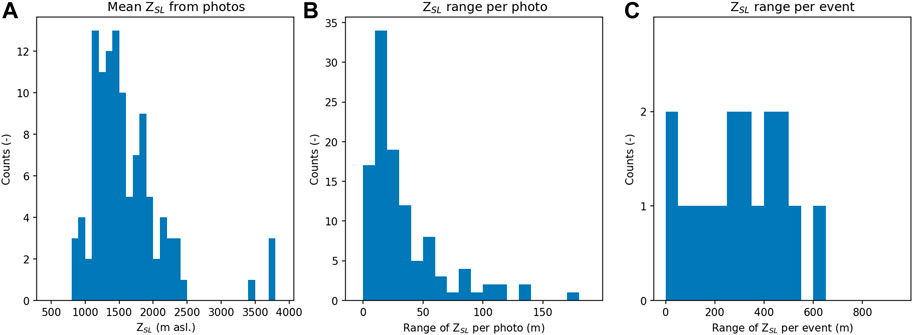
FIGURE 4. Histograms of the distribution of (A) mean ZSL from all photos, (B) maximum minus minimum ZSL per photo, and (C) range of maximum minus minimum mean ZSL per event with ≥3 photos available.
Most photos show a maximum range of <50 m between the highest and lowest estimation of ZSL (Figure 4B). Only for seven photos, this difference is ≥100 m. The estimation of ZSL with photographic evidence seems, therefore, quite robust. For events documented by at least three photos (Figure 4C), most photographs show a variation of the highest and lowest ZSL estimation ranging between 0 and 500 m. This difference could be a result of spatial differences in snowpack ablation and therefore indicate the spatial variability of ZSL some hours after an event. The event with the largest difference between photos (>900 m) is from the precipitation episode in August 2015. This value must be evaluated carefully because the photos are not from the same days and thus may represent ZSL under different rainy environments. There are five events with differences of 400–700 m. Visual analysis suggests that there are north–south gradients in ZSL (being both positive and negative), and there might be slightly lower ZSL for valleys compared to foothills (∼200 m). But there are not enough photographs to identify robust systematic variations for valleys–foothills or north–south.
We then compared ZSL values from the Sentinel-2 NSDI product in the Elqui river basin area to those from the photographic evidence. In Figure 5, we found a high correlation between ZSL from satellite imagery and photographic evidence (R2 = 0.79), and the differences are, in most cases, <500 m (19 from 23 data points). Where the satellite imagery is taken more than 3 days after the photo, ZSL tends to lay significantly above ZSL from the photos after the event. This is what we expect in this subtropical region because after most precipitation events and especially on north-facing slopes, snow melts (or sublimates) quickly. Since we found a good agreement between satellite images and photos, we can conclude that photos are valuable evidence and can be used to relate Z0C estimates to the snowline.
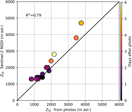
FIGURE 5. Comparison between ZSL from Sentinel-2 NSDI and photos.
In Figure 6, Z0C estimates from different methods are compared to the snowline ZSL from photos. For each panel, one point represents the results for one photo and its corresponding estimate. Figures 6A–D show a high correlation between Z0C estimates from the method M1 and ZSL from photos (R2 ≥ 0.86) if stations within 10 km are considered. As expected, the correlation slightly decreases for a larger station distance, for example, 25 km (R2 ≥ 0.77, not shown here). With steeper LRs, the standard deviation and mean offset decrease and the correlation increases (Figures 6A–D). The different lapse rates of −6.5 to −5°C km−1 yield mean offsets that correspond to threshold temperatures of 0.4–1.3°C (TSL = ZD‧LR), which is within the typical range used in the literature. Note that the mean offset in Figure 6 is only an indicator for the offset ZD between Z0C and ZSL during precipitation events (Figure 1), since it can also be influenced by local conditions at the meteorological stations used for the extrapolation techniques or the conditions of the slope such as soil temperature or vegetation type. We can also observe that there are some cases where the snowline lies up to ∼200 m above Z0C—in particular for a LR of −6.5°C km−1. There are different reasons why this might occur: First, snow could have melted away quickly within a few hours at low elevations due to warm ground or meteorological conditions. Second, some stations might be in areas where the temperature dropped during the precipitation event, while the photo was taken at a site where this did not occur or not with the same magnitude (see Section 4.2.1). There might be other explanations, but more in-situ observations would be needed to fully resolve this uncertainty.
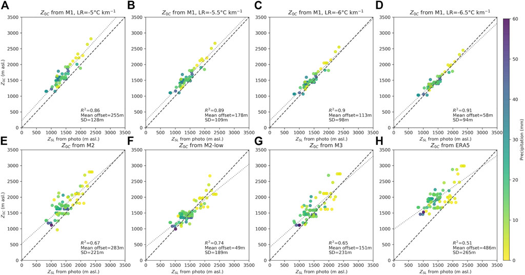
FIGURE 6. Different Z0C estimates compared to ZSL from photographic evidence: (A–D) Z0C from stations using a constant LR (method M1, only stations within 10 km); Z0C from a linear regression (E) among all stations and (F) considering only stations below 2,400 m asl. (method M2); (G) Z0C from linear interpolation between stations above/below Z0C (method M3); (H) Z0C from ERA5 reanalysis. Each data point represents one photo with its respective Z0C estimation. Note that some events are represented by up to 13 photos, and not all events are documented with photographic evidence.
The method M2 yields a moderate correlation between Z0C and ZSL if stations at high elevations are included (R2 = 0.67, Figure 6E). If only stations below 2,400 m asl. are considered (method M2-low), the correlation is higher (R2 = 0.74, Figure 6F). But more importantly, there are several cases where the snowline altitude lies more than 200 m above Z0C, which might indicate a weakness in the method M2-low. The method M3 leads to a similar correlation as M2 (Figure 6G), but there are also many cases where the snowline lies above Z0C, similar as for M2-low (Figure 6F). In contrast, the correlation between ERA5 Z0C and ZSL is smaller (R2 = 0.51, Figure 6H), and there is a considerable offset of 486 m, which indicates that ERA5 data overestimates Z0C over the mountains. This offset could occur due to the lowering effect of Z0C over mountains (Section 4.3). The standard deviation of the different methods M2, M2-low, and M3 ranges between ∼190–230 m, indicating a similar range of uncertainty of around 200 m. ERA5 has the highest standard deviation of 265 m.
We further found that the scores (R2, mean offset and standard deviation) in Figure 6 are quite sensitive to individual photos, especially the ones with a relatively high ZSL compared to the estimated Z0C. Therefore, the numbers given in Figure 6 are only indicative and serve to compare and discuss the different methods but cannot precisely quantify precisely the mean offset and standard deviation.
With the different methods presented earlier, we then estimated the typical range of minimum Z0C during precipitation days. Precipitation days are defined separately for the two regions Elqui and Limarí/Choapa when at least three stations recorded ≥2 mm, resulting in 84 and 161 days for 2011–June 2021. From these days, we selected the days where all four methods delivered a result, resulting in 70 and 139 days for Elqui and Limarí/Choapa, respectively. As expected, approximately 90% of all events occur during winter, and there are more precipitation days for the more southernly Limarí/Choapa region. We did not apply M1 here because it is difficult to compare the conditions at individual stations (due to different record periods and local conditions, see Figure 9).
Figure 7 shows the typical range for the two regions and during winter and summer. Results from the approach M2 indicate an interquartile range of ∼1830–2,490 m asl. (Elqui) and ∼1830–2,360 m asl. (Limarí/Choapa) for daily minimum Z0C (Figures 7A,B) for precipitation days during winter (May–October). As expected, the median of M2 decreases slightly by ∼130 m for Limarí/Choapa (∼2,100 m asl.) compared to Elqui (∼2,230 m asl.), most probably due to the north–south gradient (Mardones and Garreaud, 2020). In summer (Figures 7C,D), the median increases by ∼830 and 740 m for the Elqui and Limarí/Choapa regions, respectively. These numbers are approximate as there are too few days available in summer for a robust analysis. The results from the M2-low method (considering only stations <2,400 m asl.) are considerably lower, as already observed in Figures 6E,F. The difference between the median values is 310 and 630 m during winter for Elqui and Limarí/Choapa, respectively. Especially for the region Limarí/Choapa, the values below 500 m asl. seem unrealistic. A high sensitivity of Z0C estimations to high elevation stations was also described by Ibañez et al. (2020) and will be discussed in more depth in Section 4.2.3. The M3 method shows similar median values as M2. Reanalysis data from ERA5 indicate a slightly higher Z0C compared to M2 and M3, in the range of 100–400 m, depending on season and region. This result is in line with Climate Forecast System Reanalysis (CFSR) data that indicate mean rainy conditions Z0C of 2,500–2,600 between 32–30°S (Mardones and Garreaud, 2020).
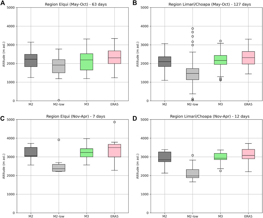
FIGURE 7. Boxplots of minimum daily Z0C during rainy days during May–October in the study region (A) Elqui and (B) Limarí/Choapa and November–April in (C) Elqui and (D) Limarí/Choapa, based on M2 (including all stations), M2-low (only considering stations <2,400 m asl.), M3, and ERA5 for 2011-June 2021. The number of days considered is given in the subplot titles.
4.2 Strengths and Limitations of the Different Methods
4.2.1 Case Studies
For every photo, we plotted the temporal evolution of hourly precipitation and Z0C from M1 (from stations within 25 km and the coastal station Nr. 17 and 6 for Elqui and Limarí/Choapa, respectively), M2, M2-low, M3, and ERA5 during the 48-h prior the photo capture. In Figures 8A,B, we present two case studies (13 July 2015 and 14 October 2015, respectively) for events with snow observed in Pisco Elqui (∼1,200 m asl.) and with some types of precipitation triggered hazards in Vicuña and surroundings (Palma, 2019). The selection represents similar findings as for the other events that are not shown here.
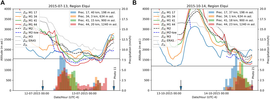
FIGURE 8. Two examples of meteorological conditions during events with photographic evidence. Bars: hourly precipitation from different meteorological stations within 25 km; lines: Z0C estimates using different methods and ERA5; horizontal line: ZSL from photo. For method M1, a LR of −6.5°C km−1 was applied. During both events, mass movements were observed in Vicuña and its surroundings, and snow was observed in Pisco Elqui (∼1,200 m asl.).
The meteorological synoptic conditions associated with the two case studies are illustrated in Supplementary Figure S5 in the supplementary information. Both events were produced by cold fronts and their associated closed-low or trough pressure systems and moisture plumes with strong water vapor transported from the Pacific Ocean. The first event (12–13 July 2015) had stronger synoptic forcings, with lower pressure depression and stronger moisture transports, and produced higher precipitation accumulation than those of the second event 2 (14 October 2015). Although both events had different precipitation and synoptic forcing intensities, both represent typical synoptic conditions with frontal systems and Pacific-originated moisture plumes reaching the subtropical coastal latitudes of the Coquimbo Region (∼30°S).
In Figure 8, we can observe a temperature decline during the two events for almost all meteorological stations located in valleys (especially 39 and 44), leading to temporal drops in Z0C from M1. The drop generally appears around the hours with the highest hourly precipitation intensities and seems less pronounced for events with low hourly intensities. In all events with snow in Vicuña, this drop appears, and this temporal drop is less clear or not visible in Z0C from M1 applied to the coastal stations. It probably occurs due to mesoscale air cooling on the upslope sector of the Andes caused mainly by diabatic cooling from the melting of orographically enhanced precipitation rates and adiabatic cooling for the upslope ascending of the air (Minder et al., 2011). But more studies are needed to identify and quantify the processes that lead to this drop in air temperature.
Z0C from linear regression and low altitude stations (<2,400 m asl., M2-low) shows similar minimum values as Z0C from M1 applied to valley stations. Z0C from linear regression, including high altitude stations, is generally higher, and the drop of Z0C is, in most cases, less pronounced. The drop is also visible in the timeline of Z0C from M3. In contrast, ERA5 reanalysis data indicate higher Z0C values compared to M1 and M2 and the temporal drop of Z0C is not clearly indicated.
4.2.2 Extrapolation of Air Temperature From Single Stations (M1)
Even if the M1 method seems suitable in most cases for nearby stations (Figures 6A-D), uncertainties are expected to increase for meteorological stations at larger distances or for certain stations due to non-elevational factors. But there is a lack of understanding about the representativeness of stations depending on their characteristics, such as elevation or surrounding topography. Also, the magnitude of the uncertainty in the function of these characteristics is not well known. Therefore, we applied a lapse rate of −6.5°C km−1 and the estimated offset ZD from Figure 6D to stations up to 50 km away from the photo using Eq. 2. Figure 9 shows the difference between ZSL from M1 and from photos, in the function of 1) distance between meteorological stations and photos and 2) station elevation.
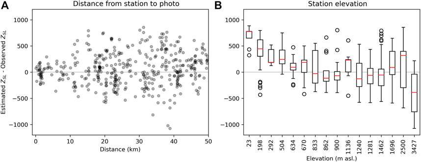
FIGURE 9. Difference between ZSL from M1 and photos, using a constant LR of −6.5°C km−1 and an offset between Z0C and ZSL of 58 m (from Figure 6D) in the function of (A) station distance and (B) station elevation. This analysis considers all stations within 50 km of each photo. Each data point represents a value for one station compared to a photo, each photo having up to 9 stations within 50 km.
In Figure 9A, we can observe that the ZSL from M1 corresponds well to ZSL from photos for close stations <10 km. The difference between the estimated and observed ZSL, however, significantly increases with a larger distance between the meteorological station to the photo. For stations >10 km away from the photographic evidence, the estimated ZSL lies in many cases more than 200 m above or below the observed ZSL, which is considerable for hydrological applications.
Uncertainty also depends on station elevation (Figure 9B). As already observed in the study cases (Figure 8), low coastal stations with elevations up to ∼500–700 m asl. tend to overestimate ZSL. The most representative stations seem to be located at ∼700–1,500 m asl. with most of the errors within ±200 m (see the interquartile range and relatively small median error in Figure 9B). These stations are located below the typical snow–rain transition zone. Comparatively, the spread of the uncertainty probably increases for higher stations (see whiskers for standard deviation), especially for stations >1,000 m asl. The study cases in Figure 8 (and more study cases not shown here) indicate that there is a strong temporal drop in Z0C for these stations. The relatively low temperatures in specific valleys and events might thus be accurate to estimate ZSL in the same valleys, but not for other sites. The relatively high-altitude stations 47 (1,696 m asl.) and 49 (2,500 m asl.) tend to overestimate ZSL. The highest station TASC (3,427 m asl.)—located clearly above the snow–rain transition zone in most cases and at large distances—probably lies too high or far for representative Z0C estimations.
We found that applying other lapse rates (−5, −5.5, and −6°C km−1) and corresponding offsets from Figures 6A–C does not change the overall pattern of the results in Figure 9 (not shown here). Our findings confirm that uniform lapse rates applied to representative and nearby (<10 km) stations might be suitable to estimate the local snowline altitude for rainy conditions if the station is located below the snow–rain transition. In Chile, wet-weather SLTR values from −5.8 to −6.2°C km−1 were found for the western subtropical Andes (Ibañez et al., 2020) and ∼−6.5°C km−1 for the coastal mountains (González and Garreaud, 2019). Even if the assumption of a uniform and constant surface lapse rate of −6.5°C km−1 is a poor one for annual mean lapse rates (Gardner and Sharp, 2009; Minder et al., 2010), we can confirm the recommendation by Ibañez et al. (2020) of using a value between −5.5 and −6.5°C km−1 to estimate minimum Z0C during rainy conditions.
4.2.3 Linear Regression Method (M2)
In Figures 6E and F, we observed that a linear regression method using surface stations at different elevations seems accurate, but the result strongly depends on the inclusion of high-elevation stations. If only stations in valley bottoms and at low altitudes (<2,400 m asl.) are considered, the extrapolated Z0C lies much lower, and in many cases, the snowline lies above Z0C. This might indicate that the method is not very precise in these cases. To understand the elevational distribution of air temperature during precipitation events, we examined the daily minimum air temperature during the six snow events in the period 2014–2021 in Pisco Elqui (Figures 10A-F). The minimum temperature is recorded at almost the same hour for all stations during these days. LR and Z0C are then calculated through the M2 method with linear regression for stations above and below 1,500 m asl. For all six events, Z0C estimated with high elevation stations lies clearly above Z0C from low elevation stations and LRs of the higher zone are less steep compared to the lower elevations. Hence, there seems to be a break in LR around the snow–rain transition, together with an offset of up to 430 m. Our findings confirm that stations from a wide range of elevations (especially high elevations) are crucial, such as suggested by Lute and Abatzoglou (2020) or Ibañez et al. (2020).
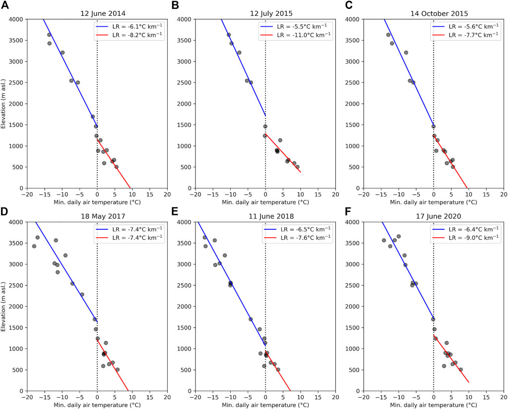
FIGURE 10. Elevation vs. minimum daily air temperature for mountain stations above 500 m asl. in the Elqui region during the six snow events at 1,200 m asl. (in Pisco Elqui). Red/blue lines show linear regressions between stations below/above 1,500 m asl.
The difference between the two Z0C values could be interpreted as a zone of an air temperature of near 0°C, called the isothermal layer (Findeisen, 1940; Unterstrasser and Zängl, 2006), which occurs if air mass in the valley becomes decoupled from the environmental flow. In this case, the latent heat required for melting the falling snow is continuously removed from the valley, thereby lowering the snow–rain transition and increasing ZD. The formation of an isothermal layer of similar magnitude has been observed and simulated for other mountainous regions (Thériault et al., 2012). This process could explain a drop in air temperature of stations in steep valleys such as observed in the study cases (Figure 8), for example, Pisco Elqui (station 44). An isothermal layer might also explain why M2 leads to higher Z0C values if high elevation stations above the isothermal layer are included. More research is needed to study the formation of isothermal layers during storm events in this region. It is also important to note that near-surface air temperature might also be altered by other local conditions. Further research could focus on the sensitivity of estimated lapse rates to single stations.
4.2.4 Linear Interpolation Between Two Stations (M3)
The interpolation technique using two stations (one below and one above Z0C) is accurate but relies on high elevation stations above the typical range of the snow–rain transition. In some cases, there is an air temperature inversion with positive air temperatures at higher elevations than negative air temperatures below. In these cases, the linear interpolation between air temperature recorded at two stations are not accurate. Similar as in M2-low, the comparison with the snowline from photos has shown many cases where the snowline lies above Z0C. This indicates that a local cooling of the atmosphere could lead to temperature drops at certain stations, which then lead to lower Z0C estimations that are not representative of the conditions of nearby valleys. But we need further studies to better understand these cases. We suggest that this method should only be applied if reliable stations are available and if local effects of temperature variability are well understood.
4.3 Mesoscale Behavior of Z0C
Since we do not have vertically pointing radars in the valleys and at the coast, it is not easy to identify the magnitude of the mesoscale lowering. We, therefore, use two simple approaches based on the methods presented above as the first attempt to assess the possible existence of the mesoscale lowering of Z0C.
4.3.1 West–East Cross Sections
The cross-barrier plot in Figure 11A shows that the 11 events present a lowering of extrapolated Z0C toward the Cordillera, with values up to 766 m. Assuming that a constant lapse rate of −6.5 C km−1 is associated with important uncertainties in the estimation of the lowering, there might also be cases where conditions at low elevations are dry and saturated aloft, leading to different LRs. To account for these uncertainties, we did the same cross-sections assuming a lapse rate of −5°C km−1 for the mountain stations (34, 41, 44, and 47), which leads to a less pronounced lowering of up to 487 m (not shown here). Still, 7 of 11 study cases present a decrease of Z0C over the mountain area compared to the coast. In contrast, cross-sections of ERA5 data do not show the lowering of Z0C. Figure 11A also shows the topography of ERA5, which seems coarse for this complex topography lying some hundreds of meters above the location of the meteorological stations.
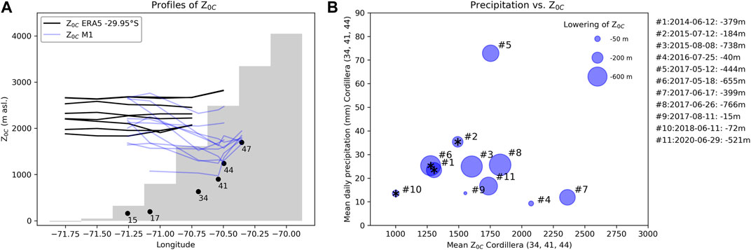
FIGURE 11. (A) Cross-sections of Z0C from ERA5 and estimated based on coast stations (15 and 17) and lapse rates from radiosonde profiles and stations in the Cordillera (34, 41, 44, and 47) based on a lapse rate of −6.5°C km−1. The grey area shows the ERA5 topography. (B) Difference (size of the circle) between Z0C from the mountainside (34 and 41) and coast stations (15 and 17) in function of daily precipitation and minimum air temperature (34 and 41) for the same dates as in (A). Snowflake symbols indicate days with snow observed in Pisco Elqui (near station 44).
Figure 11B suggests that the differences in the mountainside and upwind Z0C may accentuate with higher precipitation intensities, but more data are needed to further investigate this relationship. A dependency on precipitation intensity would be in line with observations (Marwitz 1983) and analytical models (Unterstrasser and Zängl, 2006) that have been used to understand how higher precipitation intensities lead to more latent cooling from melting precipitation and deeper isothermal 0°C layers.
An alternative interpretation of this result is that above the location of valley stations, an isothermal layer forms with temperatures slightly above 0°C and with very low air temperature gradients within that layer (Figure 1, Findeisen, 1940; Unterstasser and Zaengl, 2006), which is supported by the findings in Figure 10. At stations 44 and 47, temperatures slightly above 0°C are recorded for most precipitation events, despite the station elevation difference of 456 m. When we apply constant lapse rates of, for example, −6.5°C km−1 to these low air temperatures, the extrapolated Z0C lies a few 100 m above ground at both locations. However, if there is an isothermal layer with air temperatures slightly above 0°C and Z0C at its top, a constant LR of, for example, −6.5°C km−1 is only valid up to the bottom of the isothermal layer, and the top of the isothermal layer lies at a much higher altitude. This would then result in a much less significant lowering of Z0C over the mountains. If this is true, we underestimate Z0C significantly using ground stations located below an isothermal layer and standard LR, even if ZSL estimations seem accurate (Figure 6).
Based on this analysis, we cannot conclude whether this drop in extrapolated Z0C is due to a mesoscale lowering of Z0C or an isothermal layer, or both. In any case, it indicates that during precipitation events, there are either mesoscale lowering in Z0C or locally changed lapse rates due to isothermal layers that need to be considered to estimate the snow–rain transition altitude, especially if we base the estimation on radiosonde stations from the coast or reanalysis data. Due to these effects, the local snow–rain transition seems to be much lower than estimated based on the conditions at the coast, although an offset could be added to account for the lowering or the isothermal layer.
4.3.2 ERA5 vs. Linear Regression of Station Data
In Section 4.3.1, we were unable to quantify the mesoscale drop in Z0C, as constant LRs (M1) might underestimate Z0C if an isothermal layer forms. In contrast, Z0C estimates using linear regression (M2) with in situ stations might lead to more robust Z0C estimates. Since we found that ERA5 Z0C is well correlated with radiosonde records, we assume that these data may also be representative along the coast of the Coquimbo Region. A large difference between ERA5 and mountainside Z0C might therefore indicate a mesoscale lowering of Z0C over the Cordillera.
Figure 12 shows that the two values (Z0C from M2 representing the mountainside and ERA5 data representing the coast) are well correlated (R2 = 0.69 and 0.66 for Elqui and Limarí/Choapa), but there is an offset in the range of 150–160 m, which may indicate a mesoscale lowering. For the snow events in Pisco Elqui (see snowflake symbols in Figure 12A), the offset even increases to 297 m. The results are in line with observations from the Sierra Nevada, where an average drop of the snow–rain transition of 170 m was identified using 3 years of profiling radar observations over the windward slopes (Minder and Kingsmill, 2013). For example, Thériault et al. (2015) have shown using WRF model simulations that Z0C decreased by 400 m within 60 min until reaching the ground in the Pacific Coast Ranges. The difference between the two regions might be due to the different properties of the incoming flow or topography, which all have effects on the mesoscale lowering (Minder et al., 2011). Since the lowering is the result of a complex interplay between humidity, wind speed, stratification, air temperature, and topography, more research is needed to understand regional differences along the Chilean Andes.
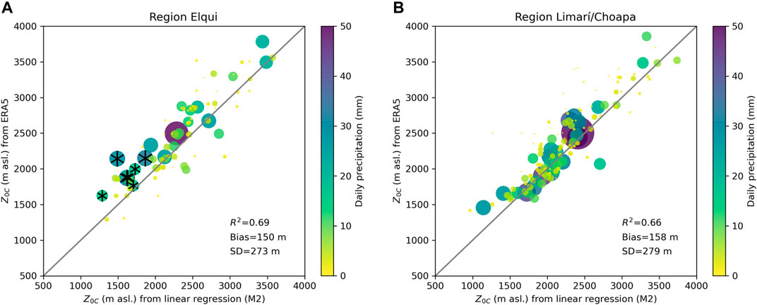
FIGURE 12. Scatterplots of ERA5 Z0C vs. Z0C during precipitation events from M2 for the regions (A) Elqui and (B) Limarí/Choapa. Snowflake symbols indicate days with snow observed in Pisco Elqui (∼1,200 m asl.). Note that the values are daily minimum Z0C during rainy hours recorded at the two reference stations, 44 and 39 for Elqui and Limarí/Choapa, respectively. Daily precipitation is also taken from these reference stations.
5 Conclusion and Recommendations
The snow–rain transition altitude is a key factor for hydrometeorological and glaciological processes in mountainous regions. Therefore, a proper estimation of the snow–rain transition is crucial for road security, agriculture, and flood alerts. In this work, we used photographs taken by participants of a citizen science programme as ground truth for the altitude of the snowline. We found that photographs of the mountain snowline after precipitation events are in good agreement with Sentinel-2 NSDI imagery and have great potential to validate empirical ZSL estimations. We first evaluated different traditional methods to estimate Z0C and ZSL based on surface station data along the upslopes of the Andes and ERA5 reanalysis data. The different methods were then used to evaluate the typical range of Z0C during precipitation events, and corresponding strengths and limitations were discussed and related to local meteorological processes such as isothermal layers. Then, the possible existence of mesoscale lowering of Z0C over the mountains with respect to that in the free atmosphere upstream of the Andes was assessed.
We can confirm that the here presented methods (M1, M2, and M3) are quite accurate, computationally efficient, and can be used for applications such as weather forecasting and flood alerts. Despite some limitations, the different methods (especially M2, including high elevation stations and M3) enable the estimation of the typical range of Z0C during precipitation events. The results from method M2 indicate an interquartile range of Z0C of ∼1830–2,490 m asl. (Elqui) and ∼1830–2,360 m asl. (Limarí/Choapa) for precipitation days during winter (May–October). ZSL is expected at an average of ∼280 m below Z0C, but this offset is only approximate and cannot be directly transferred to other methodologies since it depends on the data availability and a diversity of other local factors (such as the formation of isothermal layers, local temperature drops, and soil temperature). The different methods to estimate Z0C during precipitation events can be summarized as follows:
• If there are nearby meteorological stations, the traditional approach (M1) assuming constant LRs (−5 to −6.5°C km−1) and corresponding threshold temperatures is quite accurate to estimate ZSL during precipitation events over a certain catchment. We found that minimum air temperature during precipitation hours is a good predictor for ZSL (except during events with increasing snow–rain transition during the last precipitation hours). Our results indicate that different LRs lead to similarly high correlations, but the threshold temperature or offset ZD needs to be adapted accordingly to estimate ZSL. The station location should be evaluated carefully since low altitude stations (<700 m asl.) with maritime influence and high-elevation stations above the snow–rain transition tend to overestimate ZSL. Ideally, the station lies a few hundred meters below the snow–rain transition and close to the point of interest. For larger distances >10 km between the meteorological station and the photographic evidence, the errors increase in many cases up to ±200 m. We also suggest that this method might be robust for ZSL but probably underestimates Z0C if isothermal layers with near 0°C form.
• The results indicate that—in general—the linear regression method (M2) is accurate for estimating ZSL. However, the result strongly depends on the availability of high elevation stations above the snow–rain transition altitude, achieving significantly higher estimates if high-elevation stations are considered. Without this information, the estimated Z0C and ZSL are probably lowered by local valley effects (such as isothermal layers) and need careful interpretation. We suggest that the method M2 is more accurate for estimating Z0C, while M2-low is more related to ZSL.
• An interpolation technique (M3) using two stations (one below and one above Z0C) is accurate, similar to M2. But the method strongly relies on high elevation stations above the typical range of the snow–rain transition.
• Z0C from ERA5 reanalysis data lies almost 500 m above the mountainside ZSL from photographic evidence, probably because the coarse model topography does not allow the formation of local or mesoscale effects over mountainous areas such as isothermal layers near 0°C or lowering.
Our results suggest that the mesoscale lowering of Z0C from the coast to the mountain during a frontal storm is, on average, ∼150 m, which is similar to that observed in other mountainous regions (Minder and Kingsmill, 2013). For days with intense precipitation, the data indicate a lowering of up to 700 m (in line with Minder and Kingsmill, 2013). However, it must be noted that there is considerable uncertainty in our estimates of the lowering of Z0C due to unknown vertical air temperature lapse rates, which makes it difficult to properly compare our results with other studies. In situ meteorological data also point to the formation of a wide isothermal layer with near-freezing temperatures and shallow lapse rates. However, air temperature at the meteorological stations might also be influenced by other local effects and needs careful interpretation.
Both the effects, isothermal layers and lowering, can cause snowfall in valley bottoms, even if the upwind Z0C lies up to 500 m higher than the local snowline. This has implications for different methods to estimate Z0C and ZSL, but more data is needed to isolate and quantify these effects. Since the observed lowering is large enough to have implications for runoff, future research should focus on high-resolution numerical modeling, such as the Weather Research and Forecasting (WRF) modeling, to study the vertical structure of precipitation events and to quantify the mesoscale lowering and its dependence on, for example, topography, precipitation intensity, wind speed, humidity, and stability of the atmosphere and/or air temperature. Experimental radiosonde observations during selected storms and real-time Doppler radar observations at selected sites (upwind and in valleys) would be useful to shed light on the questions discussed here (Massmann et al., 2017).
As there is a need for more detailed studies about the future upward shift of the snow–rain transition altitude (Espinoza et al., 2020), we recommend installing stations around the typical range of snow–rain transition to study and monitor the air temperature evolution during precipitation events at different elevations. In the case of the Coquimbo Region, additional meteorological stations would be useful between 1,000 and 2,500 m asl. Photos after precipitation events are valid in situ information of the snowline altitude and should therefore be included in citizen science projects in mountainous areas. Since the manual evaluation is very time-intensive, we recommend considering automated mapping techniques.
Data Availability Statement
The original contributions presented in the study are included in the article/Supplementary Material; further inquiries can be directed to the corresponding author.
Author Contributions
SS: Conceptualization, data curation, formal analysis, funding acquisition, investigation, methodology, project administration, visualization, and writing. GP: Data curation, methodology, and writing—review. SM: Funding acquisition, supervision, and writing—review. ÁA: Formal analysis, writing—original draft preparation, writing—review, and conceptualization. MV: Conceptualization, methodology, writing—review and editing, investigation, and visualization.
Funding
SS was funded by the Swiss National Science Foundation Grant nr. P2ZHP2_187765. SM was funded by ANID-CENTROS REGIONALES R20F0008.
Conflict of Interest
The authors declare that the research was conducted in the absence of any commercial or financial relationships that could be construed as a potential conflict of interest.
Publisher’s Note
All claims expressed in this article are solely those of the authors and do not necessarily represent those of their affiliated organizations, or those of the publisher, the editors, and the reviewers. Any product that may be evaluated in this article, or claim that may be made by its manufacturer, is not guaranteed or endorsed by the publisher.
Acknowledgments
Sentinel imagery was downloaded from the EO Browser (https://apps.sentinel-hub.com/eo-browser). CEAZA station data are available at http://www.ceazamet.cl. ERA5 data are accessible through https://cds.climate.copernicus.eu. Upper air sounding data can be downloaded at https://www.ncei.noaa.gov/products/weather-balloon/integrated-global-radiosonde-archive. ÁA acknowledges FONDECYT-Postoc 3190732. We also acknowledge the project REDES of IANIGLA-CEAZA (ANID REDES-180099). Most of this work was performed with open and free languages and software (QGIS, Python). The authors thank all participants from the programme “Vecinos de las Nieves”: V. Aliste, P. Nuñez, J. Alcayaga, C. Araya, C. Canihuante, D. Canihuante, L. Canihuante, M. Carmona, C. Cortés, M. Díaz, M. Gómez, A. Muñiz, G. Oporto, C. Peralta, A. Pizarro, C. Rojas, J. C. Silva y, and J. Torres. They thank Marcela Zavala, Patricio Jofré, and Janina Guerrero for assisting the social media campaign. They thank all the people that also sent them photos from the snowline: R. Araya, F. Arce, C. Astudillo, J. Carvajal, J. Córdova, J. Larrain, C. Manzano, K. Meléndez, S. Munizaga, M. Palleros, M. Piñones, D. Pizarro, M. Quiñones, K. Rojas, A. Sandoval, C. Sirvent, B. Tapia, M. Tapia, E. Toro, R. Villalobos y, and J. V. Río Elqui. They also thank the authors of the photos that they found on social networks: Portales de INIA Intihuasi, Multimedia Ovalle TV, Elqui Semanario, El Vicuñense, El Paihuanino, El Comunal, El Hurtadino, El Andacollino, Aguslepe en Flickr, F. Barraza, M. Collao, A. Cortés, P. Díaz, M. González, M. Huerta, P. Jofré, M. López, R. Orrego, L. Ponce, J. C. Robles, R. Rojas, S. Smith, E. Toro, J. Yáñez y, and V. Velásquez. The authors would also like to thank the two reviewers for their critical and constructive comments that have enabled significant improvements to the paper.
Supplementary Material
The Supplementary Material for this article can be found online at: https://www.frontiersin.org/articles/10.3389/feart.2022.875795/full#supplementary-material
References
Alvarez-Garreton, C., Mendoza, P. A., Boisier, J. P., Addor, N., Galleguillos, M., Zambrano-Bigiarini, M., et al. (2018). The CAMELS-CL Dataset: Catchment Attributes and Meteorology for Large Sample Studies - Chile Dataset. Hydrol. Earth Syst. Sci. 22, 5817–5846. doi:10.5194/hess-2018-2310.5194/hess-22-5817-2018
AMS (2021). AMS Glossary. 2nd ed. Boston: American Meteorological Society. Retrieved from: http://amsglossary.allenpress.com/glossary/browse.
Blandford, T. R., Humes, K. S., Harshburger, B. J., Moore, B. C., Walden, V. P., and Ye, H. (2008). Seasonal and Synoptic Variations in Near-Surface Air Temperature Lapse Rates in a Mountainous Basin. J. Appl. Meteorology Climatol. 47 (1), 249–261. doi:10.1175/2007JAMC1565.1
CEAZA (2021). Vecinos de las Nieves. Retrieved from: http://cienciaciudadana.ceaza.cl. Accessed on 22 March 2021.
Copernicus Climate Change Service (2017). ERA5: Fifth Generation of ECMWF Atmospheric Reanalyses of the Global Climate. U. K. Copernic. Clim. Change Serv. Clim. Data Store (CDS). Retreived from: https://cds.climate.copernicus.eu/cdsapp#!/home. Accessed on 22 March 2021.
Cui, G., Bales, R., Rice, R., Anderson, M., Avanzi, F., Hartsough, P., et al. (2020). Detecting Rain-Snow-Transition Elevations in Mountain Basins Using Wireless Sensor Networks. J. Hydrometeorol. 21 (9), 2061–2081. doi:10.1175/JHM-D-20-0028.1
Espinoza, J. C., Garreaud, R., Poveda, G., Arias, P. A., Molina-Carpio, J., Masiokas, M., et al. (2020). Hydroclimate of the Andes Part I: Main Climatic Features. Front. Earth Sci. 8 (64), 1–20. doi:10.3389/feart.2020.00064
European Space Agency (2022). Level-2A Algorithm Overview. European Space Agency. Avilable on https://sentinels.copernicus.eu/web/sentinel/technical-guides/sentinel-2-msi/level-2a/algorithm.
Fabry, F., and Zawadzki, I. (1995). Long-Term Radar Observations of the Melting Layer of Precipitation and Their Interpretation. J. Atmos. Sci. 52, 838–851. doi:10.1175/1520-0469
Falvey, M., and Garreaud, R. D. (2009). Regional Cooling in a Warming World: Recent Temperature Trends in the Southeast Pacific and along the West Coast of Subtropical South America (1979-2006). J. Geophys. Res. 114, D04102. doi:10.1029/2008jd010519
Favier, V., Falvey, M., Rabatel, A., Praderio, E., and López, D. (2009). Interpreting Discrepancies between Discharge and Precipitation in High-Altitude Area of Chile's Norte Chico Region (26-32°S). Water Resour. Res. 45 (2), 1-20. doi:10.1029/2008WR006802
Findeisen, W. (1940). The Formation of the 0°C Isothermal Layer in Fractocumulus and Nimbostratus. Meteorol. Z. 57, 49–54.
Froidurot, S., Zin, I., Hingray, B., and Gautheron, A. (2014). Sensitivity of Precipitation Phase over the Swiss Alps to Different Meteorological Variables. J. Hydrometeorol. 15 (2), 685–696. doi:10.1175/JHM-D-13-073.1
Gardner, A. S., and Sharp, M. (2009). Sensitivity of Net Mass-Balance Estimates to Near-Surface Temperature Lapse Rates when Employing the Degree-Day Method to Estimate Glacier Melt. Ann. Glaciol. 50, 80–86. doi:10.3189/172756409787769663
Garreaud, R. D., Alvarez-Garreton, C., Barichivich, J., Boisier, J. P., Christie, D., Galleguillos, M., et al. (2017). The 2010-2015 Megadrought in Central Chile: Impacts on Regional Hydroclimate and Vegetation. Hydrol. Earth Syst. Sci. 21, 6307–6327. doi:10.5194/hess-21-6307-2017
Garreaud, R. D., Boisier, J. P., Rondanelli, R., Montecinos, A., Sepúlveda, H. H., and Veloso‐Aguila, D. (2020). The Central Chile Mega Drought (2010-2018): A Climate Dynamics Perspective. Int. J. Climatol. 40 (1), 421–439. doi:10.1002/joc.6219
Garreaud, R. (2013). Warm Winter Storms in Central Chile. J. Hydrometeorol. 14, 1515–1534. doi:10.1175/JHM-D-12-0135.1
Gascoin, S., Grizonnet, M., Bouchet, M., Salgues, G., and Hagolle, O. (2019). Theia Snow Collection: High-Resolution Operational Snow Cover Maps from Sentinel-2 and Landsat-8 Data. Earth Syst. Sci. Data 11 (2), 493–514. doi:10.5194/essd-11-493-2019
González, S., and Garreaud, R. (2019). Spatial Variability of Near-Surface Temperature over the Coastal Mountains in Southern Chile (38°S). Meteorol. Atmos. Phys. 131 (1), 89–104. doi:10.1007/s00703-017-0555-4
Harpold, A. A., Kaplan, M. L., Klos, P. Z., Link, T., McNamara, J. P., Rajagopal, S., et al. (2017). Rain or Snow: Hydrologic Processes, Observations, Prediction, and Research Needs. Hydrol. Earth Syst. Sci. 21 (1), 1–22. doi:10.5194/hess-21-1-2017
Hersbach, H., Bell, B., Berrisford, P., Hirahara, S., Horányi, A., Muñoz‐Sabater, J., et al. (2020). The ERA5 Global Reanalysis. Q.J.R. Meteorol. Soc. 146 (730), 1999–2049. doi:10.1002/qj.3803
Ibañez, M., Gironás, J., Oberli, C., Chadwick, C., and Garreaud, R. D. (2020). Daily and Seasonal Variation of the Surface Temperature Lapse Rate and 0°C Isotherm Height in the Western Subtropical Andes. Int. J. Climatol. 41, 1-20. doi:10.1002/joc.6743
Immerzeel, W. W., Petersen, L., Ragettli, S., and Pellicciotti, F. (2014). The Importance of Observed Gradients of Air Temperature and Precipitation for Modeling Runoff from a Glacierized Watershed in the Nepalese Himalayas. Water Resour. Res. 50, 2212–2226. doi:10.1002/2013WR014506
Jara, F., Lagos-Zúñiga, M., Fuster, R., Mattar, C., and McPhee, J. (2021). Snow Processes and Climate Sensitivity in an Arid Mountain Region, Northern Chile. Atmosphere 12 (4), 520. doi:10.3390/atmos12040520
JAXA (2011). Dataset ALOS PALSAR. Retrieved from: https://search.asf.alaska.edu/. Accessed on 22 March 2021.
Knowles, N., Dettinger, M. D., and Cayan, D. R. (2006). Trends in Snowfall versus Rainfall in the Western United States. J. Clim. 19 (18), 4545–4559. doi:10.1175/JCLI3850.1
Lagos-Zúñiga, M. A., and Vargas-Mesa, X. (2014). Potenciales influencias del cambio climático en crecidas pluviales en una cuenca andina. Tecnol. Ciencias Del. Agua. 5 (2), 19–38. Retrieved from http://www.scielo.org.mx/scielo.php?script=sci_arttext&pid=S2007-24222014000200002&lang=pt.
Liu, J., Chen, R., and Wang, G. (2015). Snowline and Snow Cove Monitoring at High Spatial Resololution in a Mountainous River Basin Based on a Time-Lapse Camera at Daily Scale. J. Mt. Sci. 12 (2), 60–69. doi:10.1007/s11629-013-2842-y
Lundquist, J. D., Neiman, P. J., Martner, B., White, A. B., Gottas, D. J., and Ralph, F. M. (2008). Rain versus Snow in the Sierra Nevada, California: Comparing Doppler Profiling Radar and Surface Observations of Melting Level. J. Hydrometeorol. 9 (2), 194–211. doi:10.1175/2007JHM853.1
Lute, A. C., and Abatzoglou, J. T. (2020). Best Practices for Estimating Near‐surface Air Temperature Lapse Rates. Int. J. Climatol. 41 (S1), E110–E125. doi:10.1002/joc.6668
Mardones, P., and Garreaud, R. D. (2020). Future Changes in the Free Tropospheric Freezing Level and Rain-Snow Limit: The Case of Central Chile. Atmosphere 11, 1–16. doi:10.3390/atmos11111259
Marwitz, J. D. (1983). The Kinematics of Orographic Airflow during Sierra Storms. J. Atmos. Sci. 40, 1218–1227. doi:10.1175/1520-0469(1983)040<1218:tkooad>2.0.co;2
Massmann, A. K., Minder, J. R., Garreaud, R. D., Kingsmill, D. E., Valenzuela, R. A., Montecinos, A., et al. (2017). The Chilean Coastal Orographic Precipitation Experiment: Observing the Influence of Microphysical Rain Regimes on Coastal Orographic Precipitation. J. Hydrometeorol. 18 (10), 2723–2743. doi:10.1175/JHM-D-17-0005.1
Matsuo, T., and Sasyo, Y. (1981). Melting of Snowflakes below Freezing Level in the Atmosphere. J. Meteorol. Soc. Jpn. 59 (1), 10–25. doi:10.2151/jmsj1965.59.1_10
Medina, S., Smull, B. F., Houze, R. A., and Steiner, M. (2005). Cross-barrier Flow during Orographic Precipitation Events: Results from MAP and IMPROVE. J. Atmos. Sci. 62 (10), 3580–3598. doi:10.1175/JAS3554.1
Minder, J. R., and Kingsmill, D. E. (2013). Mesoscale Variations of the Atmospheric Snow Line over the Northern Sierra Nevada: Multiyear Statistics, Case Study, and Mechanisms. J. Atmos. Sci. 70 (3), 916–938. doi:10.1175/JAS-D-12-0194.1
Minder, J. R., Mote, P. W., and Lunquist, J. D. (2010). Surface Temperature Lapse Rates over Complex Terrain: Lessons from the Cascade Mountains. J. Geophys. Res. 115, 1-13. doi:10.1029/2009jd013493
Minder, J. R., Durran, D. R., and Roe, G. H. (2011). Mesoscale Controls on the Mountainside Snow Line. J. Atmos. Sci. 68 (9), 2107–2127. doi:10.1175/JAS-D-10-05006.1
Palma, G. (2019). Análisis y cartografía de procesos geológicos peligrosos en Vicuña, Región de Coquimbo. Chile: Universidad de Atacama, Facultad de Ingeniería, Departamento de Geología. Unpublished thesis.
Portenier, C., Hüsler, F., Härer, S., and Wunderle, S. (2020). Towards a Webcam-Based Snow Cover Monitoring Network: Methodology and Evaluation. Cryosphere 14, 1409–1423. doi:10.5194/tc-2019-14210.5194/tc-14-1409-2020
Prein, A. F., and Heymsfield, A. J. (2020). Increased Melting Level Height Impacts Surface Precipitation Phase and Intensity. Nat. Clim. Chang. 10 (8), 771–776. doi:10.1038/s41558-020-0825-x
Réveillet, M., MacDonell, S., Gascoin, S., Kinnard, C., Lhermitte, S., and Schaffer, N. (2020). Impact of Forcing on Sublimation Simulations for a High Mountain Catchment in the Semiarid Andes. Cryosphere 14 (1), 147–163. doi:10.5194/tc-14-147-2020
Rutllant, J., and Fuenzalida, H. (1991). Synoptic Aspects of the Central Chile Rainfall Variability Associated with the Southern Oscillation. Int. J. Climatol. 11 (1), 63–76. doi:10.1002/joc.3370110105
Saavedra, F., Cortés, G., Viale, M., Margulis, S., and McPhee, J. (2020). Atmospheric Rivers Contribution to the Snow Accumulation over the Southern Andes (26.5° S-37.5° S). Front. Earth Sci. 8, 1–11. doi:10.3389/feart.2020.00261
Scaff, L., Rutllant, J. A., Rahn, D., Gascoin, S., and Rondanelli, R. (2017). Meteorological Interpretation of Orographic Precipitation Gradients along an Andes West Slope Basin at 30°S (Elqui Valley, Chile). J. Hydrometeorol. 18 (3), 713–727. doi:10.1175/JHM-D-16-0073.1
Schaefli, B., Hingray, B., Niggli, M., and Musy, A. (2005). A Conceptual Glacio-Hydrological Model for High Mountainous Catchments. Hydrol. Earth Syst. Sci. 9, 95–109. doi:10.5194/hessd-2-73-200510.5194/hess-9-95-2005
Schauwecker, S., Rohrer, M., Huggel, C., Endries, J., Montoya, N., Neukom, R., et al. (2017). The Freezing Level in the Tropical Andes, Peru: An Indicator for Present and Future Glacier Extents. J. Geophys. Res. Atmos. 122, 5172–5189. doi:10.1002/2016JD025943
Seidel, D. J., Sun, B., Pettey, M., and Reale, A. (2011). Global Radiosonde Balloon Drift Statistics. J. Geophys. Res. 116 (7), 1-8. doi:10.1029/2010JD014891
Sumargo, E., Cannon, F., Ralph, F. M., and Henn, B. (2020). Freezing Level Forecast Error Can Consume Reservoir Flood Control Storage: Potentials for Lake Oroville and New Bullards Bar Reservoirs in California. Water Resour. Res. 56 (8), 1–13. doi:10.1029/2020WR027072
Thériault, J. M., Rasmussen, R., Smith, T., Mo, R., Milbrandt, J. A., Brugman, M. M., et al. (2012). A Case Study of Processes Impacting Precipitation Phase and Intensity during the Vancouver 2010 Winter Olympics. Weather Forecast. 27 (6), 1301–1325. doi:10.1175/WAF-D-11-00114.1
Thériault, J. M., Milbrandt, J. A., Doyle, J., Minder, J. R., Thompson, G., Sarkadi, N., et al. (2015). Impact of Melting Snow on the Valley Flow Field and Precipitation Phase Transition. Atmos. Res. 156, 111–124. doi:10.1016/j.atmosres.2014.12.006
Unterstrasser, S., and Zängl, G. (2006). Cooling by Melting Precipitation in Alpine Valleys: An Idealized Numerical Modelling Study. Q. J. R. Meteorol. Soc. 132 (618), 1489–1508. doi:10.1256/qj.05.158
Vergara Dal Pont, I. P., Santibañez Ossa, F. A., Araneo, D., Ferrando Acuña, F. J., and Moreiras, S. M. (2018). Determination of Probabilities for the Generation of High-Discharge Flows in the Middle Basin of Elqui River, Chile. Nat. Hazards 93 (1), 531–546. doi:10.1007/s11069-018-3313-0
Viale, M., and Nuñez, M. N. (2011). Climatology of Winter Orographic Precipitation over the Subtropical Central Andes and Associated Synoptic and Regional Characteristics. J. Hydrometeorol. 12 (4), 481–507. doi:10.1175/2010JHM1284.1
Viale, M., Houze, R. A., and Rasmussen, K. L. (2013). Upstream Orographic Enhancement of a Narrow Cold-Frontal Rainband Approaching the Andes. Mon. Weather Rev. 141 (5), 1708–1730. doi:10.1175/MWR-D-12-00138.1
Viale, M., Valenzuela, R., Garreaud, R. D., and Ralph, F. M. (2018). Impacts of Atmospheric Rivers on Precipitation in Southern South America. J. Hydrometeorol. 19 (10), 1671–1687. doi:10.1175/JHM-D-18-0006.1
Virman, M., Bister, M., Räisänen, J., Sinclair, V. A., and Järvinen, H. (2021). Radiosonde Comparison of ERA5 and ERA-Interim Reanalysis Datasets over Tropical Oceans. Tellus A Dyn. Meteorol. Oceanogr. 73 (1), 1–7. doi:10.1080/16000870.2021.1929752
White, A. B., Gottas, D. J., Strem, E. T., Ralph, F. M., and Neiman, P. J. (2002). An Automated Brightband Height Detection Algorithm for Use with Doppler Radar Spectral Moments. J. Atmos. Ocean. Technol., 19, 6872–7697. doi:10.1175/1520-0426(2002)019<0687:aabhda>2.0.co;2
Keywords: 0°C isotherm, freezing level, melting level, precipitation, snow–rain transition, citizen science, dry subtropical Andes, ERA5 data
Citation: Schauwecker S, Palma G, MacDonell S, Ayala Á and Viale M (2022) The Snowline and 0°C Isotherm Altitudes During Precipitation Events in the Dry Subtropical Chilean Andes as Seen by Citizen Science, Surface Stations, and ERA5 Reanalysis Data. Front. Earth Sci. 10:875795. doi: 10.3389/feart.2022.875795
Received: 14 February 2022; Accepted: 12 May 2022;
Published: 24 June 2022.
Edited by:
Alexandre M. Ramos, University of Lisbon, PortugalReviewed by:
Justin Minder, University at Albany, United StatesAnna Wilson, University of California, San Diego, United States
Copyright © 2022 Schauwecker, Palma, MacDonell, Ayala and Viale. This is an open-access article distributed under the terms of the Creative Commons Attribution License (CC BY). The use, distribution or reproduction in other forums is permitted, provided the original author(s) and the copyright owner(s) are credited and that the original publication in this journal is cited, in accordance with accepted academic practice. No use, distribution or reproduction is permitted which does not comply with these terms.
*Correspondence: Simone Schauwecker, c2ltb25lLnNjaGF1d2Vja2VyQGNlYXphLmNs