 Yang Yang1
 Lingzhi Xie
94% of researchers rate our articles as excellent or good
Learn more about the work of our research integrity team to safeguard the quality of each article we publish.
Find out more
ORIGINAL RESEARCH article
Front. Earth Sci., 18 March 2022
Sec. Structural Geology and Tectonics
Volume 10 - 2022 | https://doi.org/10.3389/feart.2022.873715
This article is part of the Research TopicQuantitative Characterization and Engineering Application of Pores and Fractures of Different Scales in Unconventional ReservoirsView all 24 articles
Hydraulic fracturing is a key technology for shale gas production. Activating the natural fracture (NF) system in shale reservoirs and forming a complex fracture network can greatly improve the effect of fracturing. The effect of fracturing is mainly influenced by geological factors and operational parameters of a reservoir. Effectively reforming a reservoir under unfavourable geological conditions and maximizing the activation of NFs in the reservoir can substantially increase its reformed volume and the production of shale gas. Alternating fluid injection (AFI) fracturing technologies using multiple fracturing fluids with different viscosities can activate closed NFs while retaining the high conductivity of the principal fracture to achieve a larger stimulated reservoir volume (SRV). In this paper, a hydraulic-mechanical coupling finite element method (FEM) of a reservoir is established, and AFI fracturing technology is numerically simulated using the continuum method. In addition, the fracture propagation stage and path propagation for AFI technology are discussed. The results show that AFI fracturing technology can form principal fractures with high conductivity and activate NFs in a reservoir to form comparatively complex fracture propagation paths.
Unconventional reservoirs such as shale, sandstone, and coal are rich in natural gas resources (Yin et al., 2020; Guo et al., 2021). Enhancing the extraction of shale gas demands successful reservoir stimulation treatment due to the low permeability characteristics of shale rock (Li, 2020; Zhao P. et al., 2021). Hydraulic fracturing and horizontal well technology are currently the most widely used shale gas exploitation technologies (Weng, 2015; Yin and Ding, 2018). There are many natural fractures (NFs) in shale reservoirs (Gale et al., 2014; Wang et al., 2020) that strongly influence the effect of reservoir stimulation on hydraulic fracturing (He et al., 2020). Making full use of the NF system and forming a complex fracture network in a reservoir can achieve a larger stimulated reservoir volume (SRV) and reservoir permeability (Mayerhofer et al., 2010; Zhao et al., 2020a).
When hydraulic fractures (HFs) propagate and encounter NFs in the reservoir, the following three behaviours occur: HFs offset along NFs, HFs cross NFs, and HFs are arrested by NFs (Sarmadivaleh, 2012). The interaction of these behaviour modes is influenced by geological factors, such as in situ stress differences, NF dip angles and NF tensile strengths, and operational parameters, such as the fracturing fluid viscosity and injection rate (Zhang et al., 2020b). In hydraulic fracturing tests, the in situ stress difference and approach angle are the most studied influencing factors. Blanton (1982) studied the influence of in situ stress and approach angle on the interaction between HFs and NFs and proposed an interaction criterion including these two factors. Warpinski and Teufel (1987) conducted a triaxial hydraulic fracturing test and suggested a criterion that includes the approach angle, stress difference and shear slip of NFs, which can predict the interaction behaviour mode of HFs and NFs. Renshaw and Pollard (1995) introduced an interaction criterion of frictional NFs and HFs at orthogonal angles, and Gu et al. (2012) expanded this criterion to nonorthogonal fractures. The mechanical properties of NFs also affect the interaction between HFs and NFs. Zhou et al. (2008) included the shear slippage of pre-existing fractures to investigate the interaction between HFs and pre-existing fractures based on the work of (Blanton, 1982). However, when the geological conditions of a reservoir are not suitable for activating NFs by conventional methods, special hydraulic fracture design is critical to activating NFs and forming complex fracture networks in hydraulic fracturing. Therefore, research on fracturing fluid viscosity and injection rate is gradually increasing. Chuprakov et al. (2014) proposed an analytical model, referred to as OpenT, of fluid penetration that describes the influence of fluid viscosity and injection rate on the interaction of HFs and NFs. He et al. (2015) confirmed through hydraulic fracturing tests that high-viscosity fracturing fluids and high injection rates tend to penetrate rather than activate natural fractures. Zou et al. (2016) indicated that low-viscosity fracturing fluid is more likely to enter NFs through computerized tomography (CT) scanning of shale samples after hydraulic fracturing, thereby forming a complex network of fractures. However, for reservoirs where it is difficult to achieve large SRVs, a variety of fracturing fluids with different viscosities are used for multi-stage fracturing (Duan et al., 2019; Cao et al., 2020; Chen G. B. et al., 2021; Wang and Wang, 2021), and research on multi-stage fracturing with multiple fluids has begun. Alternating Fluid Injection (AFI) technology is a fracturing technology that uses different fracturing fluids at different stages of multi-stages fracturing, aiming to transform geological conditions that are not conducive to the formation of complex fracture networks (Gao et al., 2021b; Fan et al., 2021; Fan et al., 2022). Hou et al. (2019) proposed a technology of alternating injection of fluids with different viscosities, which improved the activation of NFs under conditions that were not conducive to the formation of complex fracture networks (such as high differential stress). According to these experiments, using sequenced hydraulic fracturing and multiple fracturing fluids with different viscosities is a promising technology.
However, the experimental methods are limited by accuracy and sample size (Zhang et al., 2020a; Lan et al., 2021; Yang et al., 2021), and it is difficult to evaluate the fracturing effect of variable viscosity alternating injection technology. Large-scale simulations of hydraulic fracturing can obtain the whole fracture morphology and quantitative analysis of SRV changes. Therefore, it is appropriate to use numerical methods to study alternating injection technology. Numerical methods can be divided into continuum approaches and discontinuity approaches according to the description of fractures. In the discontinuity approaches, fractures are described as geometric discontinuities where fluid flows to simulate fracture propagation. Discrete element method (DEM) is suitable method for simulating hydraulic fracturing of rock reservoirs, which can clearly show the fracture propagation path and the final fracture network shape (Yoon et al., 2017; Gao, 2021a). Zhai et al. (2020) used the cohesive zone model to study the propagation of HFs in random natural fracture shale reservoirs under different working conditions. Zhao H. et al. (2021) applied the discrete fracture network model (DFN) to study the propagation of carbon dioxide fracturing networks in shale reservoirs and analysed the influence of different natural fracture densities on the shape of the fracture network. Rezaei et al. (2019) used the boundary element method (BEM) to study the propagation of the fracture network in a large-scale two-dimensional reservoir model with many natural fractures and focused on the influence of NF dip on the expansion of the fracture network. In the continuum method, the extended finite element method (XFEM) was adopted to simulate fracture propagation by adding discontinuous displacement degrees of freedom to describe the fracture width and other properties (Vahab et al., 2019; Zheng et al., 2020a). Although the extended finite element method provides visual descriptions of fractures in the continuum model, it is difficult for researchers to embed natural fractures using this method, and the calculation efficiency is not high. The smeared crack model based on the finite element method (FEM) offers a practical balance between calculation efficiency and accuracy and is easy for researchers to embed fracture into this model (Bazant and Oh, 1983). In the FEM, fractures are simplified as anisotropic damage elements. Therefore, the propagation of these fractures is expressed as damage zones, and this method has adequate efficiency to study the interaction between HFs and NFs (Tang et al., 2018; Zhao Z. et al., 2020).
Although there are many studies on the fracture propagation process of hydraulic fracturing, most of them consider only the injection of one type of fracturing fluid, and research on the alternate injection of multiple fracturing fluids of different viscosities is very rare. Therefore, it is of practical significance to simulate the stimulation effect of alternating fluid injection multi-stage fracturing technology through numerical methods and to observe the final fracture network morphology. In this paper, an FEM model of a shale reservoir with an embedded fracture is established to simulate the interaction between HFs and NFs and explore the effect of alternating injection of fracturing fluids with different viscosities on the SRV and the maximum capability of this technology.
In the FEM model of hydraulic-mechanical coupling, shale is treated as a porous material according to the extended formula of Biot’s consolidation theory (Zienkiewicz and Shiomi, 1984). The fracturing fluid in the shale is treated as a single-phase flow.
The mass balance differential equation of shale is as follows:
where
According to the principle of effective stress, the relationship between effective stress and total stress is as follows:
where
The effective stress is the force applied on a rock skeleton, which determines the elastic strain of the rock, and its relationship is as follows:
where
The geometric equation including the relationship between strain and displacement is as follows:
where
According to the mass conservation relationship of fluid flow, the following equation can be obtained:
where
Fluid flow conforms to Darcy’s law, and the relationship between flow flux and pore pressure is as follows:
where
The compressibility parameter in Eq. 5 can be calculated as follows:
where
According to the model of initiation, fractures can be divided into toughness-dominated fractures and viscosity-dominated fractures. For the continuous model whose mesh size is much larger than the fracture tip, viscosity-dominated fractures are usually used to simulate the initiation of fractures, that is, when the elelemnt stress exceeds the corresponding strength, fractures are generated (Zhou, 2013; Li et al., 2016). In this case, the strength criterion is suitable for determining rock failure. In this paper, the anisotropic maximum tensile stress criterion is used to determine the initiation and propagation of fractures.
For a shale matrix, the failure planes of the material can be described as follows:
where
The strength of natural fractures in shale is lower than that of the matrix, and the failure plane of natural fractures can be obtained by the following formula:
where
When HF propagates in a rock matrix, the propagation direction is usually perpendicular to the direction of the maximum principal stress of the shale formation. In some cases, a single rock element includes multiple failure surfaces, and the failures of these surfaces do not affect each other (Figure 1A). In each time step, the program checks whether the stress element meets the failure criterion. Generally, the stress element is subject to the following conditions: ① The minimal principle effective stress exceeds the critical tensile stress; and ② the normal effective stress exceeds the NF tensile strength. The cases of the resulting fractures are as follows: 1) When only condition ① is satisfied, the fracture is along the direction of maximum principal stress; 2) when only condition ② is satisfied, the fracture is along the preset NF direction; and 3) when both ① and ② are satisfied at the same time, the fracture in the element can be decomposed into two fractures in specific directions (Figure 1C).
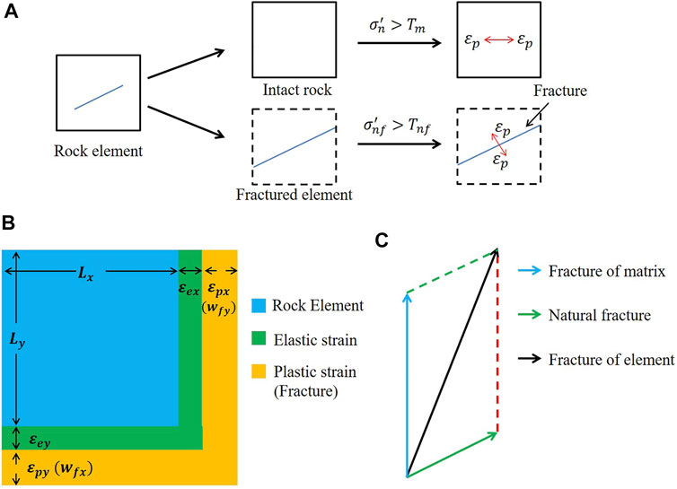
FIGURE 1. (A) Fractures in the continuum model; (B) Relationship between fracture width and plastic strain; (C) Fracture direction in a fractured element.
In Section 2.2, the plastic strain and deformation after material failure can be obtained. However, it is necessary to link the material strain with the fluid parameters to achieve a complete HF propagation fluid mechanics coupling process. When the shale is still intact rock, fluid flows in the pores of the rock and can be described by Darcy’s law. In the fracturing process, due to the low permeability of shale, fluid flow is blocked, resulting in an uneven distribution of rock pore pressure; that is, there is a difference in pore pressure between the injection point and the surrounding area. When the pressure difference accumulates to a certain value, i.e., the effective stress reaches the failure strength, the rock is damaged, and the permeability of the rock element is divided into two parts: the permeability of the fracture and the permeability of the porous medium.
Obviously, it is necessary to calculate the equivalent fracture width in order to calculate the permeability. Based on the equivalent continuum method, the strain of fractured rock consists of fracture strain and intact rock strain. The deformation of intact rock can be approximated as elastic strain, while plastic strain is completely caused by fracture deformation. Therefore, the fracture width corresponds to the result of the continuum model (Figure 1B) shown in the following equation:
where
To clearly distinguish the permeability of fractures and pores, several assumptions must be made. First, when rock breaks, the permeability of the pores remains unchanged. The increase in the permeability of the shale element is entirely the result of the initiation and expansion of fractures. Thus, based on the cubic law of fluid flow, the relationship between the equivalent permeability and fracture width can be established:
where
This program is a secondary development based on the above theories and methods on the ANSYS® platform. First, the reservoir parameters are input, and a reservoir model with a natural fracture is built. Then, fluid is injected into the reservoir for fracturing, and whether the shale rock material breaks is determined. If a rock element of the reservoir is damaged, then the material permeability corresponding to this element is updated for the subsequent calculation. The program continues to loop through these steps until the entire fracturing process is completed.
Fracture and reservoir properties can be easily obtained using numerical methods, allowing the fracturing effect to be quantified. The total area of the reservoir fracture network and the SRV are two indicators that are used frequently for measuring the effect of reservoir fracturing.
The SRV is commonly used as the standard for measuring the effect of stimulation in shale reservoirs. It is calculated by using the discrete bins method (Mayerhofer et al., 2010), which packs the fracture elements into several bins with a fixed width and a certain length to approximately calculate the SRV (Figure 2) using the equation below:
where
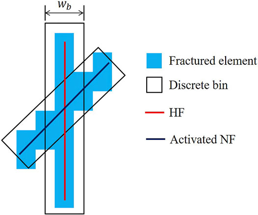
FIGURE 2. Discrete bins method for the SRV calculation.
The fracture network permeability, which corresponds to reservoir permeability and hydraulic fracture conductivity, is another method for evaluating the fracturing effect (Ofoegbu and Smart, 2019). The total fracture network permeability is computed as follows:
where
In the FEM, the fractures are treated as damage elements instead of discontinuities, which prevents the propagation path and properties of the fractures in the continuous model from being clearly displayed. In this paper, to visually display the fractures in the FEM, two assumptions are made: 1) The propagation direction of HFs in the shale matrix element is perpendicular to the direction of the maximum plastic strain of the element (Figure 3A); and 2) in the elements with NFs, the plastic strain is decomposed into the direction of the minimum principal stress and the direction perpendicular to the NF (Figure 3B). In addition to the above assumptions, some fractures are corrected and merged in this process.
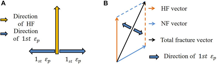
FIGURE 3. Schematic of hydraulic fracture visualization (A) In elements without NFs; (B) In elements with NFs.
In this section, the correspondence between the numerical model and the true triaxial hydraulic fracturing test is verified.
Experiments are commonly used to determine the reliability of numerical models before simulations are conducted. The focus of this article is the interaction between HFs and NFs. Therefore, experiments related to the interaction of fractures are selected to verify the validity of the model. Gu et al. (2012) used silicone oil as the fracturing fluid in actual triaxial hydraulic fracturing tests (Figure 4A) and studied the interaction between hydraulic fractures and natural fractures in a sandstone sample with a single pre-existing fracture. In order to correspond to the boundary conditions of the test, a two-dimensional FEM model of the horizontal in-situ stress plane was established and a pre-exist fracture was embedded (Figure 4B). And, the parameters used in Gu’s experiment are shown in Table 1. In addition to the parameters in Table 1, other basic parameters are used in this model, which are listed in Table 2.
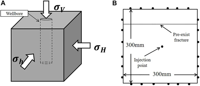
FIGURE 4. (A) Schematic diagram of the hydraulic fracturing sample; (B) the FEM model used in the verification.
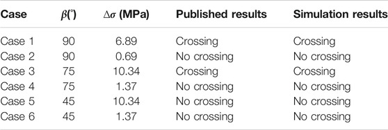
TABLE 1. Parameters used in Gu’s actual triaxial hydraulic fracturing experiment.
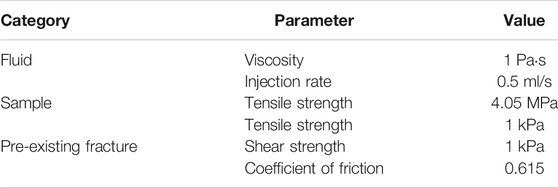
TABLE 2. Parameters used in the model validation.
To verify the numerical model, a 300 mm × 300 mm two-dimensional hydraulic fracturing model is established. A natural fracture is embedded in the model, which is consistent with the experiment. For fracturing, a concentrated fluid is injected into the model’s centre. The HFs gradually approaches the NFs, leading to one of two results: crossing or no crossing.
Where β is approaching angle, which is the angle between the propagation direction of hydraulic fracture and the direction of natural fracture; Δσ is in-situ stress difference, which is equal to (σ1–σ3).
In this paper, a numerical model with the same parameters as the experimental model of Gu et al. (2012) is used to simulate fracture interaction, and the equivalent fracture width results are shown in Figure 5. However, to ensure the convergence of the FEM simulation, a small value, 1 kPa, is used instead of 0 for the strength of the pre-existing fracture.
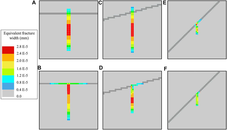
FIGURE 5. Width of HF (A) Case 1, (B) Case 2, (C) Case 3, (D) Case 4, (E) Case 5 and (F) Case 6.
As shown in Figure 5, the interaction between HFs and NFs is divided into two situations: Crossing or no crossing. In detail, Cases 1 (Figure 5A) and 3 (Figure 5C) cross, and Cases 2, 4, 5 and 6 (Figures 5B,D–F) do not cross. In addition, the colours of the elements in Figure 5 indicate the widths of different fractures, which are calculated by equation (8). The light grey area in Figure 5 represents the intact part of the matrix, and the dark grey band represents the inactive pre-existing fracture.
After verification, the results of the interaction between HFs and NFs based on the continuum method are consistent with the results of the actual triaxial hydraulic fracturing experiment. Therefore, this model can effectively simulate the interaction between HFs and NFs and obtain accurate results.
In this section, the hydraulic fracturing simulation is conducted with the validated hydraulic fracturing numerical model to study the influence of fluid viscosity on the effects of fracturing. To fully demonstrate the role of viscosity, this section is divided into the following parts: Section 4.1 describes the establishment of the engineering-scale hydraulic fracturing FEM model and its boundary conditions. Section 4.2 studies the influence of different viscosities on fracture interactions. Section 4.3 introduces the alternating fluid injection (AFI) technology process and discusses how it improves the fracture interaction mode. Section 4.4 studies the influence of AFI technology on the fracturing of the reservoir.
There are natural fractures of different scales in shale reservoirs, including micro-fractures (Figure 6A), macro-fractures in samples (Figure 6B), and large-scale fractures in shale reservoirs (Figure 6C). Micro-fractures and sample-scale fractures affect the mechanical properties of the rock, while large-scale fractures in the reservoir affect the direction of HF propagation and the final fracture network morphology. To simulate the propagation of HF in shale reservoirs with NFs, a large-scale reservoir model is built to perform engineering-scale numerical simulations of shale hydraulic fracturing.
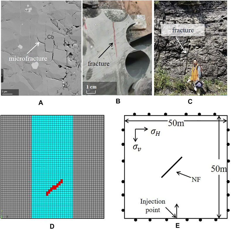
FIGURE 6. (A) micro-fracture (Chen J. et al., 2021); (B) sample-scale fracture; (C) large-scale fracture (Zheng et al., 2020b); (D) FEM model of fractured reservoir; (E) boundary condition of reservoir model.
As shown in Figure 6D, the size of the FEM model of the reservoir is 50 × 50 m. The grey elements are permeable and without fractures which represents an area not affected by fracturing. The middle blue area represents the part of the reservoir affected by fracturing, and the red elements represent the embedded NF. Notably, if the angle of the NF differs, then the position of the red element also differs. Figure 6D shows only the case where the NF dip angle is 45°. In the model, there are 2,500 fluid mechanical coupled elements, including 984 rock matrix elements, 16 NF elements and 1,500 elements for the simulation of seepage.
As shown in Figure 6E, the model applies normal displacement and pore pressure constraints to the four sides of the reservoir. To simulate the real formation situation, initial in situ stresses in the horizontal direction and vertical direction are applied, and the in situ stresses are balanced. After hydraulic fracturing start, a concentrated fluid load is applied to the reservoir and acts on the element at the boundary to simulate fluid injection. The parameters used in the simulation are shown in Table 3.
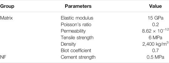
TABLE 3. Parameters of the reservoir model.
The numerical simulation cases were divided into single fluid injection fracturing and AFI cases. The simulation cases and parameters are listed in Table 4.
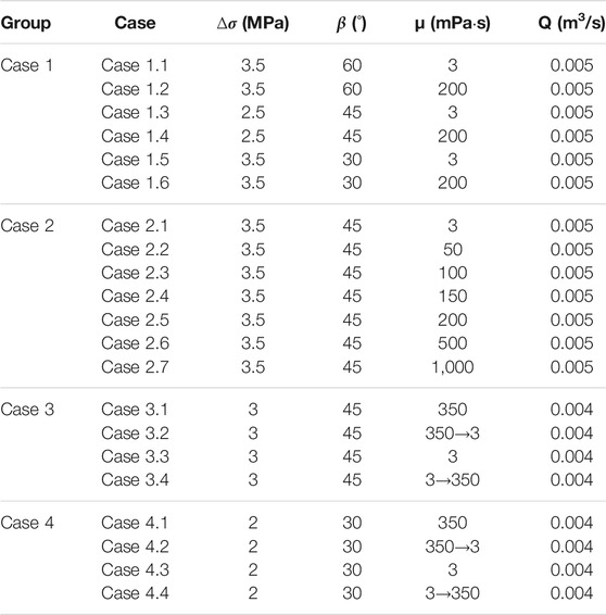
TABLE 4. List of cases used in this paper.
In this section, the role of fracturing fluid viscosity in fracturing is discussed from the aspects of fracture morphology and evaluation of the reservoir stimulation effect.
The viscosity of the fracturing fluid is the main parameter that can be controlled. Viscosity is a physical quantity that measures frictional resistance during fluid flow. High-viscosity fluid has great resistance in the direction of flow, and it is difficult for it to enter the pores of shale. In contrast, low-viscosity fluid tends to enter the NFs in shale due to its low resistance during flow, thereby accumulating pressure in the NFs and activating them.
Figure 7 shows the equivalent fracture width of HFs for different viscosities and approach angles. From top to bottom, the approach angles are 60°, 45°, and 30°. In Figures 7A,C,E, high-viscosity fracturing fluids are used; in Figures 7B,D,F, the parameters of the fracturing fluid are those of water. Figure 7 clearly shows that when the viscosity of the fracturing fluid is relatively high, the HFs pass the NF without activating it; when the viscosity is low, the HFs propagate along the NF, offset, and increase the complexity of the fracture network.
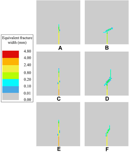
FIGURE 7. Fracture equivalent width contours: (A) Case 1.1, (B) Case 1.2, (C) Case 1.3, (D) Case 1.4, (E) Case 1.5, and (F) Case 1.6.
However, the fracture manifestation in Figure 7 does not show the fracture propagation path and fracture network shape. Therefore, according to the method in Section 2.6, the fracture equivalent width illustration is transformed into the fracture propagation path diagram shown in Figure 8.
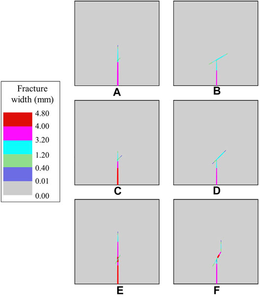
FIGURE 8. Fracture width and propagation path in hydraulic fracturing: (A) Case 1.1, (B) Case 1.2, (C) Case 1.3, (D) Case 1.4, (E) Case 1.5, and (F) Case 1.6.
In addition, the viscosity can affect the properties of the fracture, such as the fracture width. Although analytical models such as the Kristianovich-Geertsma-de Klerk (KGD) model give the relationship between the width of 2-D HFs and viscosity, they are suitable only for short fractures. Figure 9 shows fracture width vs. viscosity of some commonly used fracturing fluids; the HF width increases with increasing viscosity.
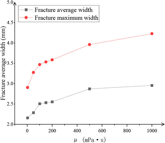
FIGURE 9. HF width curve with viscosity.
Alternating fluid injection technology is used in this paper to stimulate reservoirs with unfavourable formation parameters. AFI is usually divided into three stages: Stage 1, the use of high-viscosity fracturing fluid to fracture the reservoir (Figure 10A); stage 2, HFs pass through the NFs and expands mainly in the direction of the maximum principal stress (Figure 10B); and stage 3, continuous injection of replacement fluid, i.e., low-viscosity fracturing fluid, activates the NFs, and a more complex fracture network forms (Figure 10C). Figure 10 shows this complete process.
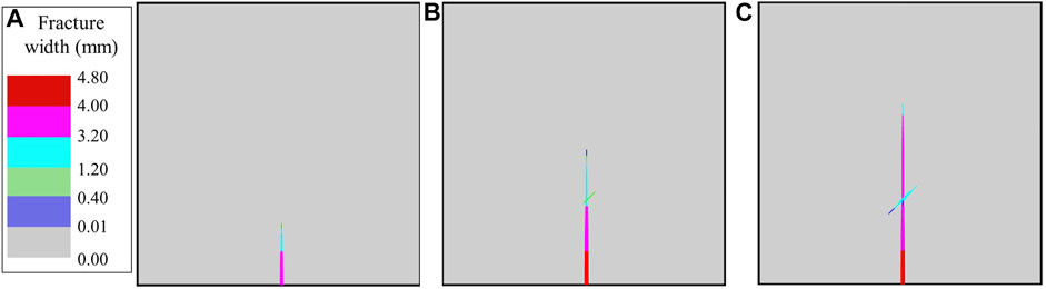
FIGURE 10. Fracture width for AFI technology: (A) stage 1, (B) stage 2, and (C) stage 3.
As shown in Figure 10, the HFs formed by the high-viscosity fracturing fluid approach and pass through the NFs; then, the low-viscosity fracturing fluid is injected in the NFs. Subsequently, the expansion of the NFs resumes, and the shapes of the HFs become more complicated. As a result, fracturing through AFI technology can not only obtain fractures with stronger conductivity but also activate NFs to form a complex fracture network.
To demonstrate the effect of AFI, this article conducts a set of control experiments, namely, fracturing with high-viscosity fracturing fluid; AFI technology with a sequence from high- to low-viscosity fluid; fracturing with low-viscosity fracturing fluid; and fracturing with a sequence from low- to high-viscosity fluid. The final fracture paths are shown in Figure 10.
Figure 11 shows the final fracture path of the reservoir with a NF with dip angle of 45°. It can be seen that the fracture length is longest in the case of the high-viscosity fracturing fluid (Figure 11A), but the SRV is narrow. The two cases of low-viscosity fracturing fluid (Figure 11C) and the sequence from low-viscosity to high-viscosity fracturing fluid (Figure 11D) are similar. And for the sequence from low-viscosity to high-viscosity fracturing fluid, the main fracture does not pass through the NFs and the length of fracture is shortest. The AFI technology that switches from high-viscosity to low-viscosity fluid (Figure 11B) simultaneously produces the longest main fracture and the largest SRV. In addition, there are three potential expansion directions for the fracture network after AFI fracturing, which greatly increases the potential of forming a complex fracture network.
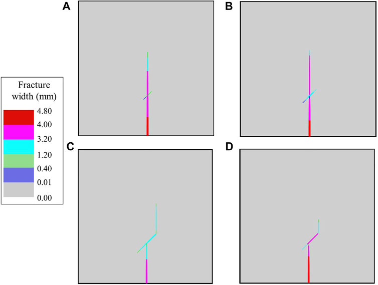
FIGURE 11. Fracture width and path of the reservoir with a NF with dip angle of 45°: (A) 350 mPa·s, (B) 350→3 mPa·s, (C) 3 mPa·s, and (D) 3→350 mPa·s.
Figure 12 shows the final fracture path of the reservoir with a NF with dip angle of 30°. Similarly, fractures created by high-viscosity fracturing fluids (Figure 12A) have ideal length and width, but lower SRV; fractures created by low-viscosity fracturing fluids (Figure 12C) can activate NF, but have smaller fracture widths. A sequence from low- to high-viscosity produces fracture with shortest length (Figure 12D). The HF fractured by AFI technology has crossed and dilated NF (Figure 12B), which keeps relatively large fracture width simultaneously.
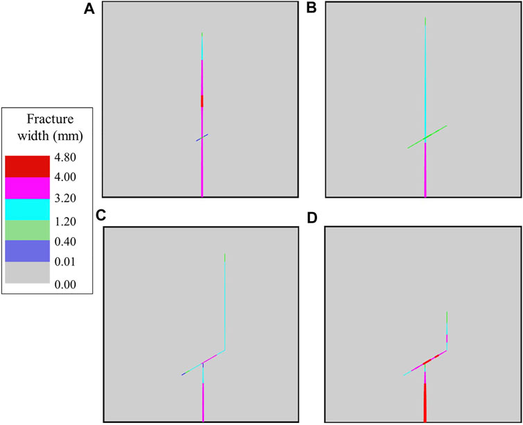
FIGURE 12. Fracture width and path of the reservoir with a NF with dip angle of 30°: (A) 350 mPas, (B) 350→3 mPa·s, (C) 3 mPa·s, and (D) 3→350 mPa·s.
The viscosity of the fracturing fluid has a considerable impact on fracture properties, and it is an important operating parameter that can be manually controlled. When evaluating the effect of reservoir stimulation, two indicators, the SRV and reservoir permeability, are commonly used. Figure 13 shows the SRV and reservoir permeability after fracturing in the four cases.
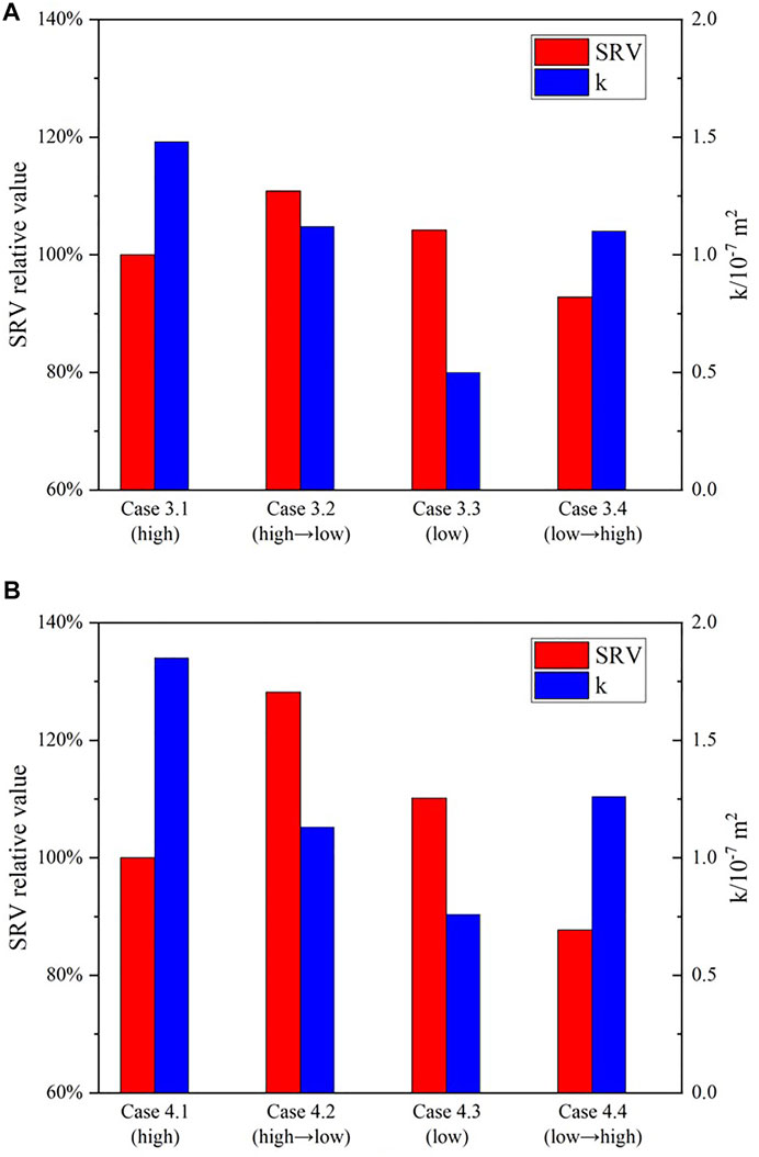
FIGURE 13. The SRV and permeability of reservoir (A) NF dip angle is 45°; (B) NF dip angle is 30°.
Figure 13A shows that compared to other fracturing technologies, AFI increases the SRV of reservoirs under the same geological conditions. Case 3.1 (high-viscosity) is set as the basis for comparison, and the SRV values of the other cases are expressed as percentages of the base value. In addition, compared with low-viscosity fracturing technology, AFI can effectively increase reservoir permeability. Compared with traditional hydraulic fracturing with high-viscosity fracturing fluid, AFI technology has the advantage of strong flow conductivity, and its permeability is almost the same as that of high-viscosity fracturing technology.
Similarly, Figure 13B shows that the SRV of the AFI technology case is significantly higher than the control high viscosity fracturing fluid case. SRV of low-viscosity fluid fracturing case is higher than the high-viscosity case but reservoir permeability is lower than the high-viscosity case. In addition, the fracturing case that switches viscosity from low to high has lowest SRV but relatively high permeability.
Combining Figures 13A,B, it can be seen that the reservoir permeability of the high-viscosity fracturing fluid case and the low-viscosity to high-viscosity fracturing fluid case are high, but the SRV are low; the low-viscosity fracturing case has comparatively high SRV but low permeability. Overall, AFI case has both the highest SRV and good reservoir permeability, and is the recommended fracturing technology.
NFs in reservoirs are potential conductivity approaches, and the effect of fracturing technology on the properties of NF is also an important indicator. To evaluate the effect of NF activation in the reservoir and the opening degree of NFs permeability are introduced. Since both the low-viscosity case and the low-to-high viscosity case fully activate NF, these two cases will be omitted from this section.
As shown in Figure 14, the NF opening degree of AFI technology (Case3.2 and 4.2) is higher than that of high-viscosity fracturing (Case3.1 and 4.1). Moreover, it can be directly found that as the dip angle decreases, the advantages of AFI technology become more obvious. It shows that AFI technology can help activate low-angle NFs in the reservoir and obtain a more complex fracture network.
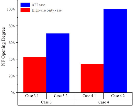
FIGURE 14. NF opening degree of the AFI and high-viscosity cases.
Figure 15 indicates that before the viscosity of the fracturing fluid changes, the NF permeability curves of the two cases overlap. After changing the viscosity, the permeability curve of AFI technology (Case3.2 and 4.2) continues to rise sharply; in contrast, the curve of the high-viscosity fluid hydraulic fracturing case (Case3.1 and 4.1) rises slowly. Obviously, compared with traditional high-viscosity fracturing technology, AFI technology can effectively activate NFs and form a complex fracture network to improve the SRV and permeability of the reservoir.
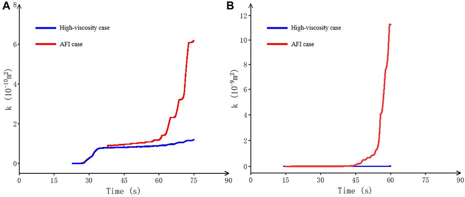
FIGURE 15. NF permeability time history curve of the AFI and high-viscosity cases (A) NF dip angle is 45°; (B) NF dip angle is 30°.
In this paper, through the secondary development of ANSYS, an FEM model of reservoir hydraulic fracturing is established. The validity of the model is verified, and hydraulic fracturing cases are simulated with different parameters.
1) The FEM has high computational efficiency and can be used to conduct numerical simulations of long-term hydraulic fracturing of engineering-scale 3D reservoirs. The traditional FEM can play a role in the numerical simulation of large-scale hydraulic fracturing.
2) Fracturing fluid viscosity has a significant effect on the width of HF. Furthermore, at different stages of fracturing, viscosity has different effects. When the NF is not opened, reducing the viscosity can activate the NF and change the interaction mode between HF and NF; while when the NF has been dilated, changing the viscosity at this time cannot change the interaction mode.
3) Numerical simulation results show that in terms of common evaluation methods such as the SRV, reservoir permeability and NF opening degree, the AFI process has obvious advantages over pure high-viscosity fracturing, pure low-viscosity fracturing and hydraulic fracturing.
4) The comparison of fracturing simulation results with different NF dip angles shows that the reservoir geological conditions are unfavorable, that is, when the NF dip angle is low, the advantages of AFI technology are more obvious.
The original contributions presented in the study are included in the article/Supplementary Material, further inquiries can be directed to the corresponding author.
YY and LX are responsible for the idea and writing of this paper and BH and PZ are responsible for the analysis.
This paper was financially supported by the National Natural Science Foundation of China (Grant No. 11872258).
The authors declare that the research was conducted in the absence of any commercial or financial relationships that could be construed as a potential conflict of interest.
All claims expressed in this article are solely those of the authors and do not necessarily represent those of their affiliated organizations, or those of the publisher, the editors and the reviewers. Any product that may be evaluated in this article, or claim that may be made by its manufacturer, is not guaranteed or endorsed by the publisher.
We are also grateful for the constructive comments from the reviewers and our editor.
Bažant, Z. P., and Oh, B. H. (1983). Crack Band Theory for Fracture of Concrete. Mat. Constr. 16, 155–177. doi:10.1007/BF02486267
Blanton, T. L. (1982). “An Experimental Study of Interaction between Hydraulically Induced and Pre-existing Fractures,” in Proceedings of the SPE Unconventional Gas Recovery Symposium, Pittsburgh, Pennsylvania, May 1982, 1–13. doi:10.2118/10847-MS
Cao, X., Wang, M., Kang, J., Wang, S., and Liang, Y. (2020). Fracturing Technologies of Deep Shale Gas Horizontal wells in the Weirong Block, Southern Sichuan Basin. Nat. Gas Industry B 7 (1), 64–70. doi:10.1016/j.ngib.2019.07.003
Chen, G. B., Li, T., Yang, L., Zhang, G. H., Li, J. W., and Dong, H. J. (2021a). Mechanical Properties and Failure Mechanism of Combined Bodies with Different Coal-Rock Ratios and Combinations. J. Mining Strata Control. Eng. 3 (2), 023522. doi:10.13532/j.jmsce.cn10-1638/td.20210108.001
Chen, J., Lan, H., Macciotta, R., Martin, C. D., and Wu, Y. (2021b). Microfracture Characterization of Shale Constrained by Mineralogy and Bedding. J. Pet. Sci. Eng. 201, 108456. doi:10.1016/j.petrol.2021.108456
Chuprakov, D., Melchaeva, O., and Prioul, R. (2014). Injection-Sensitive Mechanics of Hydraulic Fracture Interaction with Discontinuities. Rock Mech. Rock Eng. 47 (5), 1625–1640. doi:10.1007/s00603-014-0596-7
Duan, H., Li, H., Dai, J., Wang, Y., and Chen, S. a. (2019). Horizontal Well Fracturing Mode of "increasing Net Pressure, Promoting Network Fracture and Keeping Conductivity" for the Stimulation of Deep Shale Gas Reservoirs: A Case Study of the Dingshan Area in SE Sichuan Basin. Nat. Gas Industry B 6 (5), 497–501. doi:10.1016/j.ngib.2019.02.005
Fan, C., Wen, H., Li, S., Bai, G., and Zhou, L. (2022). Coal Seam Gas Extraction by Integrated Drillings and Punchings from the Floor Roadway Considering Hydraulic-Mechanical Coupling Effect. Geofluids 2022, 1–10. doi:10.1155/2022/5198227
Fan, C., Yang, L., Wang, G., Huang, Q., Fu, X., and Wen, H. (2021). Investigation on Coal Skeleton Deformation in CO2 Injection Enhanced CH4 Drainage from Underground Coal Seam. Front. Earth Sci. 9, 766011. doi:10.3389/feart.2021.766011
Gale, J. F. W., Laubach, S. E., Olson, J. E., Eichhuble, P., and Fall, A. (2014). Natural Fractures in Shale: A Review and New Observations. Bulletin 98 (11), 2165–2216. doi:10.1306/08121413151
Gao, F. (2021a). Influence of Hydraulic Fracturing of strong Roof on Mining-Induced Stress Insight from Numerical Simulation. J. Mining Strata Control. Eng. 3 (2), 023032. doi:10.13532/j.jmsce.cn10-1638/td.20210329.001
Gao, R., Kuang, T., Zhang, Y., Zhang, W., and Quan, C. (2021b). Controlling Mine Pressure by Subjecting High-Level Hard Rock Strata to Ground Fracturing. Int. J. Coal Sci. Technol. 8, 1336–1350. doi:10.1007/s40789-020-00405-1
Gu, H., Weng, X., Lund, J., Mack, M., Ganguly, U., and Suarez-Rivera, R. (2012). Hydraulic Fracture Crossing Natural Fracture at Nonorthogonal Angles: A Criterion and its Validation. SPE Prod. Oper. 27 (1), 20–26. doi:10.2118/139984-PA
Guo, L. L., Zhou, D. W., Zhang, D. M., and Zhou, B. H. (2021). Deformation and Failure of Surrounding Rock of a Roadway Subjected to Mining-Induced Stresses. J. Mining Strata Control. Eng. 3 (2), 023038. doi:10.13532/j.jmsce.cn10-1638/td.20200727.001
He, Q., Suorineni, F. T., and Oh, J. (2015). “Modeling Interaction between Natural Fractures and Hydraulic Fractures in Block Cave Mining,” in Proceedings of the 49th US Rock Mechanics/Geomechanics Symposium, San Francisco, California, June 2015.
He, X., Zhang, P., He, G., Gao, Y., Liu, M., Zhang, Y., et al. (2020). Evaluation of Sweet Spots and Horizontal-Well-Design Technology for Shale Gas in the basin-margin Transition Zone of southeastern Chongqing, SW China. Energ. Geosci. 1 (3), 134–146. doi:10.1016/j.engeos.2020.06.004
Hou, B., Chang, Z., Fu, W., Muhadasi, Y., and Chen, M. (2019). Fracture Initiation and Propagation in a Deep Shale Gas Reservoir Subject to an Alternating-Fluid-Injection Hydraulic-Fracturing Treatment. SPE J. 24 (041), 1839–1855. doi:10.2118/195571-PA
Lan, S. R., Song, D. Z., Li, Z. L., and Liu, Y. (2021). Experimental Study on Acoustic Emission Characteristics of Fault Slip Process Based on Damage Factor. J. Mining Strata Control. Eng. 3 (3), 033024. doi:10.13532/j.jmsce.cn10-1638/td.20210510.002
Li, S., Li, X., and Zhang, D. (2016). A Fully Coupled Thermo-Hydro-Mechanical, Three-Dimensional Model for Hydraulic Stimulation Treatments. J. Nat. Gas Sci. Eng. 34, 64–84. doi:10.1016/j.jngse.2016.06.046
Li, Y. (2021). Mechanics and Fracturing Techniques of Deep Shale from the Sichuan Basin, SW China. Energ. Geosci. 2 (1), 1–9. doi:10.1016/j.engeos.2020.06.002
Mayerhofer, M. J. J., Lolon, E. P. P., Warpinski, N. R. R., Cipolla, C. L. L., Walser, D., and Rightmire, C. M. M. (2010). What Is Stimulated Reservoir Volume? SPE Prod. Oper. 25 (01), 89–98. doi:10.2118/119890-PA
Ofoegbu, G. I., and Smart, K. J. (2019). Modeling Discrete Fractures in Continuum Analysis and Insights for Fracture Propagation and Mechanical Behavior of Fractured Rock. Results Eng. 4, 100070. doi:10.1016/j.rineng.2019.100070
Renshaw, C. E., and Pollard, D. D. (1995). An Experimentally Verified Criterion for Propagation across Unbounded Frictional Interfaces in Brittle, Linear Elastic Materials. Int. J. Rock Mech. Mining Sci. Geomechanics Abstr. 32 (3), 237–249. doi:10.1016/0148-9062(94)00037-4
Rezaei, A., Siddiqui, F., Bornia, G., and Soliman, M. (2019). Applications of the Fast Multipole Fully Coupled Poroelastic Displacement Discontinuity Method to Hydraulic Fracturing Problems. J. Comput. Phys. 399, 108955. doi:10.1016/j.jcp.2019.108955
Sarmadivaleh, M. (2012). “Experimental and Numerical Study of Interaction of a Pre-existing Natural Interface and an Induced Hydraulic Fracture,”. Ph.D Thesis (Perth, Australia: Curtin University).
Tang, H., Li, S., and Zhang, D. (2018). The Effect of Heterogeneity on Hydraulic Fracturing in Shale. J. Pet. Sci. Eng. 162, 292–308. doi:10.1016/j.petrol.2017.12.020
Vahab, M., Khoei, A. R., and Khalili, N. (2019). An X-FEM Technique in Modeling Hydro-Fracture Interaction with Naturally-Cemented Faults. Eng. Fracture Mech. 212, 269–290. doi:10.1016/j.engfracmech.2019.03.020
Wang, H., Shi, Z., Zhao, Q., Liu, D., Sun, S., Guo, W., et al. (2020). Stratigraphic Framework of the Wufeng-Longmaxi Shale in and Around the Sichuan Basin, China: Implications for Targeting Shale Gas. Energ. Geosci. 1 (3), 124–133. doi:10.1016/j.engeos.2020.05.006
Wang, J., and Wang, X. L. (2021). Seepage Characteristic and Fracture Development of Protected Seam Caused by Mining Protecting Strata. J. Mining Strata Control. Eng. 3 (3), 033511. doi:10.13532/j.jmsce.cn10-1638/td.20201215.001
Warpinski, N. R., and Teufel, L. W. (1987). Influence of Geologic Discontinuities on Hydraulic Fracture Propagation (Includes Associated Papers 17011 and 17074 ). J. Pet. Technol. 39 (2), 209–220. doi:10.2118/13224-PA
Weng, X. (2015). Modeling of Complex Hydraulic Fractures in Naturally Fractured Formation. J. Unconventional Oil Gas Resour. 9, 114–135. doi:10.1016/j.juogr.2014.07.001
Yang, J. X., Luo, M. K., Zhang, X. W., Huang, N., and Hou, S. J. (2021). Mechanical Properties and Fatigue Damage Evolution of Granite under Cyclic Loading and Unloading Conditions. J. Mining Strata Control. Eng. 3 (3), 033016. doi:10.13532/j.jmsce.cn10-1638/td.20210510.001
Yin, S., and Ding, W. (2018). Evaluation Indexes of Coalbed Methane Accumulation in the strong Deformed Strike-Slip Fault Zone Considering Tectonics and Fractures: a 3D Geomechanical Simulation Study. Geol. Mag. 156, 1052–1068. doi:10.1017/S0016756818000456
Yin, S., Dong, L., Yang, X., and Wang, R. (2020). Experimental Investigation of the Petrophysical Properties, Minerals, Elements and Pore Structures in Tight Sandstones. J. Nat. Gas Sci. Eng. 76, 103189. doi:10.1016/j.jngse.2020.103189
Yoon, J. S., Zang, A., Stephansson, O., Hofmann, H., and Zimmermann, G. (2017). Discrete Element Modelling of Hydraulic Fracture Propagation and Dynamic Interaction with Natural Fractures in Hard Rock. Proced. Eng. 191, 1023–1031. doi:10.1016/j.proeng.2017.05.275
Yushi, Z., Shicheng, Z., Tong, Z., Xiang, Z., and Tiankui, G. (2016). Experimental Investigation into Hydraulic Fracture Network Propagation in Gas Shales Using CT Scanning Technology. Rock Mech. Rock Eng. 49 (1), 33–45. doi:10.1007/s00603-015-0720-3
Zhai, L., Zhang, H., Pan, D., Zhu, Y., Zhu, J., Zhang, Y., et al. (2020). Optimisation of Hydraulic Fracturing Parameters Based on Cohesive Zone Method in Oil Shale Reservoir with Random Distribution of Weak Planes. J. Nat. Gas Sci. Eng. 75, 103130. doi:10.1016/j.jngse.2019.103130
Zhang, B., Shen, B., and Zhang, J. (2020a). Experimental Study of Edge-Opened Cracks Propagation in Rock-like Materials. J. Mining Strata Control. Eng. 2 (3), 033035. doi:10.13532/j.jmsce.cn10-1638/td.20200313.001
Zhang, Q., Zhang, X.-P., and Sun, W. (2021b). A Review of Laboratory Studies and Theoretical Analysis for the Interaction Mode between Induced Hydraulic Fractures and Pre-existing Fractures. J. Nat. Gas Sci. Eng. 86, 103719. doi:10.1016/j.jngse.2020.103719
Zhao, H., Wu, K., Huang, Z., Xu, Z., Shi, H., and Wang, H. (2021a). Numerical Model of CO2 Fracturing in Naturally Fractured Reservoirs. Eng. Fracture Mech. 244, 107548. doi:10.1016/j.engfracmech.2021.107548
Zhao, P., He, B., Zhang, B., and Liu, J. (2021b). Porosity of Gas Shale: Is the NMR-Based Measurement Reliable? Pet. Sci.doi:10.1016/j.petsci.2021.12.013
Zhao, P., Xie, L., Ge, Q., Zhang, Y., Liu, J., and He, B. (2020a). Numerical Study of the Effect of Natural Fractures on Shale Hydraulic Fracturing Based on the Continuum Approach. J. Pet. Sci. Eng. 189, 107038. doi:10.1016/j.petrol.2020.107038
Zhao, Z., Wu, K., Fan, Y., Guo, J., Zeng, B., and Yue, W. (2020b). An Optimization Model for Conductivity of Hydraulic Fracture Networks in the Longmaxi Shale, Sichuan basin, Southwest China. Energ. Geosci. 1 (1-2), 47–54. doi:10.1016/j.engeos.2020.05.001
Zheng, H., Pu, C., and Sun, C. (2020a). Study on the Interaction between Hydraulic Fracture and Natural Fracture Based on Extended Finite Element Method. Eng. Fracture Mech. 230, 106981. doi:10.1016/j.engfracmech.2020.106981
Zheng, H., Zhang, J., and Qi, Y. (2020b). Geology and Geomechanics of Hydraulic Fracturing in the Marcellus Shale Gas Play and Their Potential Applications to the Fuling Shale Gas Development. Energ. Geosci. 1, 36–46. doi:10.1016/j.engeos.2020.05.002
Zhou, J., Chen, M., Jin, Y., and Zhang, G.-q. (2008). Analysis of Fracture Propagation Behavior and Fracture Geometry Using a Tri-axial Fracturing System in Naturally Fractured Reservoirs. Int. J. Rock Mech. Mining Sci. 45 (7), 1143–1152. doi:10.1016/j.ijrmms.2008.01.001
Zhou, L., and Hou, M. Z. (2013). A New Numerical 3D-Model for Simulation of Hydraulic Fracturing in Consideration of Hydro-Mechanical Coupling Effects. Int. J. Rock Mech. Mining Sci. 60, 370–380. doi:10.1016/j.ijrmms.2013.01.006
Keywords: hydraulic fracturing, finite element method, alternating fluid injection, shale gas, natural fracture
Citation: Yang Y, Xie L, He B and Zhao P (2022) Numerical Study on the Use of Alternating Injection Hydraulic Fracturing Technology to Optimize the Interaction Between Hydraulic Fracture and Natural Fracture. Front. Earth Sci. 10:873715. doi: 10.3389/feart.2022.873715
Received: 11 February 2022; Accepted: 01 March 2022;
Published: 18 March 2022.
Edited by:
Shuai Yin, Xi’an Shiyou University, ChinaReviewed by:
Taotao Yan, Taiyuan University of Technology, ChinaCopyright © 2022 Yang, Xie, He and Zhao. This is an open-access article distributed under the terms of the Creative Commons Attribution License (CC BY). The use, distribution or reproduction in other forums is permitted, provided the original author(s) and the copyright owner(s) are credited and that the original publication in this journal is cited, in accordance with accepted academic practice. No use, distribution or reproduction is permitted which does not comply with these terms.
*Correspondence: Lingzhi Xie, eGllbGluZ3poaUBzY3UuZWR1LmNu
Disclaimer: All claims expressed in this article are solely those of the authors and do not necessarily represent those of their affiliated organizations, or those of the publisher, the editors and the reviewers. Any product that may be evaluated in this article or claim that may be made by its manufacturer is not guaranteed or endorsed by the publisher.
Research integrity at Frontiers
Learn more about the work of our research integrity team to safeguard the quality of each article we publish.