Wave Equation Numerical Simulation and RTM With Mixed Staggered-Grid Finite-Difference Schemes

For the conventional staggered-grid finite-difference scheme (C-SFD), although the spatial finite-difference (FD) operator can reach 2M^th-order accuracy, the FD discrete wave equation is the only second-order accuracy, leading to low modeling accuracy and poor stability. We proposed a new mixed staggered-grid finite-difference scheme (M-SFD) by constructing the spatial FD operator using axial and off-axial grid points jointly to approximate the first-order spatial partial derivative. This scheme is suitable for modeling the stress–velocity acoustic and elastic wave equation. Then, based on the time–space domain dispersion relation and the Taylor series expansion, we derived the analytical expression of the FD coefficients. Theoretically, the FD discrete acoustic wave equation and P- or S-wave in the FD discrete elastic wave equation given by M-SFD can reach the arbitrary even-order accuracy. For acoustic wave modeling, with almost identical computational costs, M-SFD can achieve higher modeling accuracy than C-SFD. Moreover, with a larger time step used in M-SFD than that used in C-SFD, M-SFD can achieve higher computational efficiency and reach higher modeling accuracy. For elastic wave simulation, compared to C-SFD, M-SFD can obtain higher modeling accuracy with almost the same computational efficiency when the FD coefficients are calculated based on the S-wave time–space domain dispersion relation. Solving the split elastic wave equation with M-SFD can further improve the modeling accuracy but will decrease the efficiency and increase the memory usage as well. Stability analysis shows that M-SFD has better stability than C-SFD for both acoustic and elastic wave simulations. Applying M-SFD to reverse time migration (RTM), the imaging artifacts caused by the numerical dispersion are effectively eliminated, which improves the imaging accuracy and resolution of deep formation.

1 Introduction

Wave equation simulation is an important technique to study the characteristics of seismic waves in complex media (Carcione, 2015; Cao and Chen, 2018), and a key kernel in reverse time migration (RTM) (Virieux et al., 2011; Berkhout, 2014) and full waveform inversion (FWI) (Pratt et al., 1998; Virieux and Operto, 2009). Compared to the pseudo-spectral method (Reshef et al., 1988; Mittet, 2021) and finite-element method (Marfurt, 1984; Moczo et al., 2010; Moczo et al., 2011), the finite-difference (FD) method has the advantage of high computational efficiency, small memory occupation and easy implementation (Alford et al., 1974; Mulder, 2017). Hence, the FD method has become the most widely used numerical method for wave propagation simulation (Alterman and Karal, 1968; Chen et al., 2021). However, the inherent numerical dispersion in FD methods seriously affects the modeling accuracy (Alford et al., 1974; Dablain, 1986) and leads to an adverse impact on RTM and FWI results (Ren et al., 2021). So suppressing the numerical dispersion to improve the modeling accuracy is an important issue for the FD method.

Dablain (1986) pointed out that approximating the temporal and spatial partial derivatives with high-order FD operators can reduce the numerical dispersion. Unfortunately, the temporal high-order FD operator significantly increases the amount of computation and decreases the stability. Hence, conventional FD (C-FD) and staggered-grid FD (C-SFD) commonly adopt temporal second-order and spatial 2M^th-order FD operators (Fornberg, 1988). With the FD coefficients calculated based on the space domain dispersion relation and Taylor series expansion (TE), the spatial FD operators in C-FD and C-SFD can achieve 2M^th-order accuracy, but the FD discrete wave equations are still only second-order accuracy (Liu and Sen, 2009). However, wave equation simulation is implemented by solving the FD discrete wave equation iteratively. So in order to improve the modeling accuracy, we should try to increase the accuracy of the FD discrete wave equation rather than improve separately the accuracy of the temporal and spatial FD operators. Liu and Sen (2009; 2011) proposed to calculate the FD coefficients of C-FD and C-SFD based on the time–space domain dispersion relation and TE, which makes the 2D and 3D FD discrete wave equations reach 2M^th-order accuracy along 8 and 48 propagation directions respectively, but the accuracy is still second-order along with the rest of the directions. In addition to the aforementioned TE methods, the least squares (LS) methods are also widely adopted for computing the FD coefficients by minimizing the error of dispersion relation, phase velocity, or group velocity (Geller and Takeuchi, 1998; Chu and Stoffa, 2012). The LS methods usually improve the accuracy of wavefield components in the medium-high frequency band but decays some accuracy of the low-frequency component. Liu (2013; 2014) found that by minimizing the relative error instead of the absolute error of space domain or time-space domain dispersion relation, the global optimal solution can be obtained without iterations.

In addition to ameliorating the method for computing the FD coefficients, constructing a more reasonable FD stencil is another important way to improve the modeling accuracy. For the 2D scalar wave equation, Liu and Sen (2013) developed a rhombus FD scheme. The FD discrete wave equation can reach 2M^th-order accuracy along with all propagation directions with the FD coefficients calculated based on the time-space domain dispersion relation. However, the length of the spatial FD operator increases rapidly with M, which makes it very computationally expensive. Wang et al. (2016) proposed an FD scheme by combining the C-FD and rhombus FD schemes, which balanced the accuracy and efficiency. Motivated by the widely used mixed-grid FD scheme in the frequency domain (Jo et al., 1996; Shin and Sohn, 1998), Hu et al. (2016) proposed a mixed-grid FD scheme for 2D scalar wave equation modeling in the time–space domain. The basic idea of Hu et al. (2016) is to express the Laplace FD operator as the weighted mean of the Laplace FD operators constructed in the general and rotated Cartesian coordinate system. The resulting mixed-grid FD scheme is similar to that of Wang et al. (2016). Hu et al. (2021) derived how to construct a 3D Laplace FD operator with the off-axial grid points and further proposed a 3D mixed-grid FD scheme, which improved the accuracy and stability of 3D scalar wave equation simulation. For the stress–velocity acoustic wave equation, Tan and Huang (2014) constructed a spatial FD operator with the axial and off-axial grid points to approximate the first-order spatial partial derivatives and developed a mixed staggered-grid FD scheme (M-SFD). This M-SFD can make the FD discrete acoustic wave equation reach fourth or sixth-order accuracy. Ren and Li (2017) extended the method of Tan and Huang (2014) to elastic wave simulation, and the accuracy of P- or S-wave in the FD discrete elastic wave equation can be up to eighth-order. However, in the M-SFD of Tan and Huang (2014) and Ren and Li (2017), two sets of off-axial grid points with different distance to the center of the spatial FD operator are sometimes assigned the same FD coefficient, which is unreasonable and makes derivation of the analytic expression of the FD coefficients too difficult.

For simulation of the stress-velocity acoustic and elastic wave equation, we intended to develop a modified M-SFD by ensuring the FD coefficient assigned to the grid points varies with their distance to the center of the spatial FD operator, which will make our M-SFD more reasonable than that of Tan and Huang (2014) and Ren and Li (2017). Then we managed to derive the analytical solution for calculating the FD coefficients with the time-space domain dispersion relation and TE. We first discretized the acoustic and elastic wave equation with our M-SFD and derived the analytical solution of the FD coefficients. This is followed by analysis of difference accuracy, numerical dispersion, and stability. Then, we performed acoustic and elastic numerical simulation on a simple three-layered model and a typical complex structural model of the Tarim Basin in Western China and compared the results of M-SFD and C-SFD. In the end, we carried out acoustic RTM with M-SFD for synthetic seismic data on the complex structural model.

2 Basic Theory of M-SFD

2.1 FD Discrete Acoustic and Elastic Wave Equation Given by M-SFD

The wavefield variables and elastic parameters are defined at staggered grid points in the staggered-grid FD scheme. Figure 1 displays the relative position of the wavefield variables and elastic parameters in acoustic and elastic staggered-grid FD schemes.

FIGURE 1

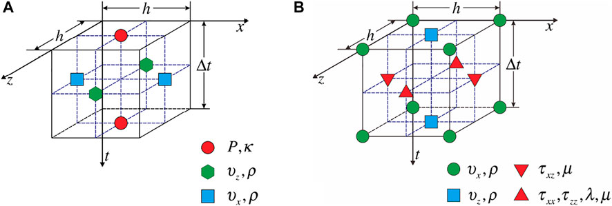
FIGURE 1. Schematic representation of the relative position of the wave-field variables and elastic parameters in (A) acoustic wave and (B) elastic wave staggered-grid FD schemes.

C-SFD adopts temporal second-order and spatial 2M^th-order FD operators. The spatial FD operator is constructed only by the axial grid points, shown in Figure 2A. In this spatial FD operator, M represents the number of sets of axial grid points with each set having the same distance to the center. As we know, M sets of grid points can ensure the spatial FD operator reaches 2M^th-order accuracy. We can also see that the distance of these points to the center of the operator increases with M, while the contribution toward improving the modeling accuracy decreases.

FIGURE 2

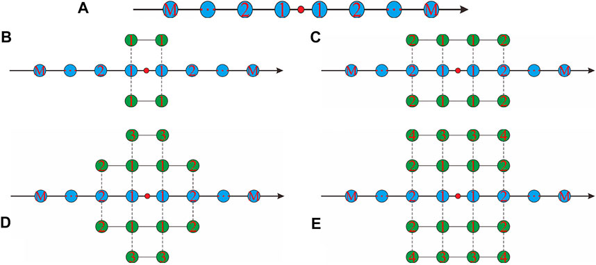
FIGURE 2. Schematic representation of the spatial FD operators of (A) C-SFD and (B–E) M-SFD (N=1, 2, 3, and 4).

In this article, we proposed a modified M-SFD by constructing the spatial FD operator using the axial and off-axial grid points while keeping the temporal second-order FD operator unchanged. In the spatial FD operators, M and N represent the number of sets of axial and off-axial grid points, respectively, and each set of grid points is equidistant from the center of the operator. The identical FD coefficient is assigned to the grid points in the same set, and different FD coefficients are assigned to different sets. Figures 2B–E show the four spatial FD operators of our M-SFD with N=1, 2, 3, and 4. Compared to C-SFD, M-SFD takes full use of the off-axial grid points near the center of the spatial FD operator.

The previous M-SFD (Tan and Huang, 2014; Ren and Li, 2017) inappropriately uses the symmetry of the off-axial grid points. Two different sets of off-axial grid points with unequal distance to the center are sometimes improperly regarded as one set and assigned the same FD coefficient. For example, in Figure 2D, the two sets of off-axial grid points labeled with ② and ③ have a different distance to the center, but the assigned FD coefficients are identical. This inappropriate assignment of the FD coefficients makes it too difficult to derive the analytical solution of the FD coefficients.

In the following, we will take M-SFD (N=1) as an example to derive the FD discrete acoustic and elastic wave equation and then derive the analytical expression of FD coefficients.

2.1.1 FD Discrete Acoustic Wave Equation

The 2D stress–velocity acoustic wave equation is given by

$\frac{\partial P}{\partial t}+\kappa \left(\frac{\partial {\upsilon }_x}{\partial x}+\frac{\partial {\upsilon }_z}{\partial z}\right)=0,\begin{array}{cc}\frac{\partial {\upsilon }_x}{\partial t}+\frac{1}{\rho }\frac{\partial P}{\partial x}=0,& \frac{\partial {\upsilon }_z}{\partial t}+\frac{1}{\rho }\frac{\partial P}{\partial z}=0,\end{array}(1)$

where $P=P\left(x,z,t\right)$ represents the pressure, ${\upsilon }_x={\upsilon }_x\left(x,z,t\right)$ and ${\upsilon }_z={\upsilon }_z\left(x,z,t\right)$ are the particle velocities, $\rho =\rho \left(x,z\right)$ represents the density, and $\kappa =\kappa \left(x,z\right)$ is the bulk modulus.

Temporal second-order FD operator to approximate $\partial P/\partial t$ is given by

${\frac{\partial P}{\partial t}|}_{1/2,1/2}^{1/2}\approx \frac{P_{1/2,1/2}^1-P_{1/2,1/2}^0}{\mathrm{\Delta }t},(2)$

where $P_{m-1/2,n-1/2}^j=P\left[x+\left(m-1/2\right)h,z+\left(n-1/2\right)h,j\mathrm{\Delta }t\right]$, and $h$ and $\mathrm{\Delta }t$ represent the grid size and time step, respectively. The spatial FD operator of M-SFD (N=1) shown in Figure 2B to approximate $\partial {\upsilon }_x/\partial x$ and $\partial {\upsilon }_z/\partial z$ is

$\begin{array}{l}{\frac{\partial {\upsilon }_x}{\partial x}|}_{1/2,1/2}^{1/2}\approx \frac{1}{h}\left\{{\displaystyle \sum _{m=1}^M{a}_m\left[{\upsilon }_{x\left(m,1/2\right)}^{1/2}-{\upsilon }_{x\left(-m+1,1/2\right)}^{1/2}\right]}+b_1\left[{\upsilon }_{x\left(1,3/2\right)}^{1/2}-{\upsilon }_{x\left(0,3/2\right)}^{1/2}+{\upsilon }_{x\left(1,-1/2\right)}^{1/2}-{\upsilon }_{x\left(0,-1/2\right)}^{1/2}\right]\right\},\\ {\frac{\partial {\upsilon }_z}{\partial z}|}_{1/2,1/2}^{1/2}\approx \frac{1}{h}\left\{{\displaystyle \sum _{m=1}^M{a}_m\left[{\upsilon }_{z\left(1/2,m\right)}^{1/2}-{\upsilon }_{z\left(1/2,-m+1\right)}^{1/2}\right]}+b_1\left[{\upsilon }_{z\left(3/2,1\right)}^{1/2}-{\upsilon }_{z\left(3/2,0\right)}^{1/2}+{\upsilon }_{z\left(-1/2,1\right)}^{1/2}-{\upsilon }_{z\left(-1/2,0\right)}^{1/2}\right]\right\},\end{array}(3)$

where $a_1,a_2,\dots ,a_M;b_1$ are the FD coefficients, ${\upsilon }_{x\left(m,n-1/2\right)}^{j-1/2}={\upsilon }_x\left[x+mh,z+\left(n-1/2\right)h,t+\left(j-1/2\right)\mathrm{\Delta }t\right]$, and ${\upsilon }_{z\left(m-1/2,n\right)}^{j-1/2}={\upsilon }_z\left[x+\left(m-1/2\right)h,z+nh,t+\left(j-1/2\right)\mathrm{\Delta }t\right]$.

Similarly, we can get the FD expressions of $\partial {\upsilon }_x/\partial t$, $\partial P/\partial x$, $\partial {\upsilon }_z/\partial t$ and $\partial P/\partial z$. Substituting the FD expressions into Eq. 1, we have

$\begin{array}{c}\frac{P_{1/2,1/2}^1-P_{1/2,1/2}^0}{\mathrm{\Delta }t}\approx -\frac{\kappa }{h}\left\{{\displaystyle \sum _{m=1}^M{a}_m\left[{\upsilon }_{x\left(m,1/2\right)}^{1/2}-{\upsilon }_{x\left(-m+1,1/2\right)}^{1/2}\right]}+b_1\left[{\upsilon }_{x\left(1,3/2\right)}^{1/2}-{\upsilon }_{x\left(0,3/2\right)}^{1/2}+{\upsilon }_{x\left(1,-1/2\right)}^{1/2}-{\upsilon }_{x\left(0,-1/2\right)}^{1/2}\right]\right\}\\ -\frac{\kappa }{h}\left\{{\displaystyle \sum _{m=1}^M{a}_m\left[{\upsilon }_{z\left(1/2,m\right)}^{1/2}-{\upsilon }_{z\left(1/2,-m+1\right)}^{1/2}\right]}+b_1\left[{\upsilon }_{z\left(3/2,1\right)}^{1/2}-{\upsilon }_{z\left(3/2,0\right)}^{1/2}+{\upsilon }_{z\left(-1/2,1\right)}^{1/2}-{\upsilon }_{z\left(-1/2,0\right)}^{1/2}\right]\right\},\\ \frac{{\upsilon }_{x\left(0,1/2\right)}^{1/2}-{\upsilon }_{x\left(0,1/2\right)}^{-1/2}}{\mathrm{\Delta }t}\approx -\frac{1}{\rho h}\left\{{\displaystyle \sum _{m=1}^M{a}_m\left(P_{m-1/2,1/2}^0-P_{-m+1/2,1/2}^0\right)}+b_1\left[P_{1/2,3/2}^0-P_{-1/2,3/2}^0+P_{1/2,-1/2}^0-P_{-1/2,-1/2}^0\right]\right\},\\ \frac{{\upsilon }_{z\left(1/2,0\right)}^{1/2}-{\upsilon }_{z\left(1/2,0\right)}^{-1/2}}{\mathrm{\Delta }t}\approx -\frac{1}{\rho h}\left\{{\displaystyle \sum _{m=1}^M{a}_m\left(P_{1/2,m-1/2}^0-P_{1/2,-m+1/2}^0\right)}+b_1\left[P_{3/2,1/2}^0-P_{3/2,-1/2}^0+P_{-1/2,1/2}^0-P_{-1/2,-1/2}^0\right]\right\},\end{array}(4)$

Equation 4 is the FD discrete acoustic wave equation given by M-SFD (N=1). Similarly, the FD discrete acoustic wave equation given by M-SFD (N=2,3,4) can be derived.

2.1.2 FD Discrete Elastic Wave Equation

The 2D stress–velocity elastic wave equation is given by

$\begin{array}{l}\begin{array}{cc}\frac{\partial {\upsilon }_x}{\partial t}=\frac{1}{\rho }\left(\frac{\partial {\tau }_{xx}}{\partial x}+\frac{\partial {\tau }_{xz}}{\partial z}\right),& \frac{\partial {\upsilon }_z}{\partial t}=\frac{1}{\rho }\left(\frac{\partial {\tau }_{xz}}{\partial x}+\frac{\partial {\tau }_{zz}}{\partial z}\right),\end{array}\\ \begin{array}{ccc}\frac{\partial {\tau }_{xx}}{\partial t}=\left(\lambda +2\mu \right)\frac{\partial {\upsilon }_x}{\partial x}+\lambda \frac{\partial {\upsilon }_z}{\partial z},& \frac{\partial {\tau }_{zz}}{\partial t}=\lambda \frac{\partial {\upsilon }_x}{\partial x}+\left(\lambda +2\mu \right)\frac{\partial {\upsilon }_z}{\partial z},& \frac{\partial {\tau }_{xz}}{\partial t}=\mu \left(\frac{\partial {\upsilon }_x}{\partial z}+\frac{\partial {\upsilon }_z}{\partial x}\right),\end{array}\end{array}(5)$

where ${\upsilon }_x={\upsilon }_x\left(x,z,t\right)$ and ${\upsilon }_z={\upsilon }_z\left(x,z,t\right)$ are the particle velocities, ${\tau }_{xx}={\tau }_{xx}\left(x,z,t\right)$, ${\tau }_{zz}={\tau }_{zz}\left(x,z,t\right)$ and ${\tau }_{xz}={\tau }_{xz}\left(x,z,t\right)$ are the stress components, $\lambda =\lambda \left(x,z\right)$ and $\mu =\mu \left(x,z\right)$ are the Lamé constants, and $\rho =\rho \left(x,z\right)$ is the density.

Similar to the derivation process of the FD discrete acoustic wave equation, the FD discrete elastic wave equation given by M-SFD (N=1) can be derived. Here, we only gave one of the five FD equations:

$\begin{array}{c}\frac{{\upsilon }_{x\left(\mathrm{0,0}\right)}^1-{\upsilon }_{x\left(\mathrm{0,0}\right)}^0}{\mathrm{\Delta }t}\approx \frac{1}{\rho h}{\displaystyle \sum _{m=1}^M{a}_m\left[\left({\tau }_{xx\left(m-1/2,0\right)}^{1/2}-{\tau }_{xx\left(-m+1/2,0\right)}^{1/2}\right)+\left({\tau }_{xz\left(0,m-1/2\right)}^{1/2}-{\tau }_{xz\left(0,-m+1/2\right)}^{1/2}\right)\right]}\\ +\frac{b_1}{\rho h}\left[\begin{array}{l}\left({\tau }_{xx\left(1/2,1\right)}^{1/2}-{\tau }_{xx\left(-1/2,1\right)}^{1/2}\right)+\left({\tau }_{xx\left(1/2,-1\right)}^{1/2}-{\tau }_{xx\left(-1/2,-1\right)}^{1/2}\right)+\\ \left({\tau }_{xz\left(1,1/2\right)}^{1/2}-{\tau }_{xz\left(1,-1/2\right)}^{1/2}\right)+\left({\tau }_{xz\left(-1,1/2\right)}^{1/2}-{\tau }_{xz\left(-1,-1/2\right)}^{1/2}\right)\end{array}\right],\end{array}(6)$

where $a_1,a_2,\dots ,a_M;b_1$ are the FD coefficients.

Using the same method, the FD discrete elastic wave equation given by M-SFD (N=2,3,4) can be derived.

2.2 FD Coefficient Calculation

2.2.1 FD Coefficient Calculation for the FD Discrete Acoustic Wave Equation

In a homogeneous medium, Eq. 1 has the following discrete plane wave solution

$\begin{array}{c}{P}_{m-1/2,n-1/2}^j=A_P{e}^{i\left[k_x\left(x+\left(m-1/2\right)h\right)+k_z\left(z+\left(n-1/2\right)h\right)-\omega \left(t+j\mathrm{\Delta }t\right)\right]},\\ {\upsilon }_{x\left(m,n-1/2\right)}^{j-1/2}=A_{{\upsilon }_x}{e}^{i\left[k_x\left(x+mh\right)+k_z\left(z+\left(n-1/2\right)h\right)-\omega \left(t+\left(j-1/2\right)\mathrm{\Delta }t\right)\right]},\\ {\upsilon }_{z\left(m-1/2,n\right)}^{j-1/2}=A_{{\upsilon }_z}{e}^{i\left[k_x\left(x+\left(m-1/2\right)h\right)+k_z\left(z+nh\right)-\omega \left(t+\left(j-1/2\right)\mathrm{\Delta }t\right)\right]},\\ \begin{array}{cc}{k}_x=k\cos \theta ,& k_z\end{array}=k\sin \theta ,\end{array}(7)$

where $A_P$, $A_{{\upsilon }_x}$, and $A_{{\upsilon }_z}$ are the plane wave amplitude factors, $k$ is the wavenumber, $\omega$ is the angular frequency, and $\theta$ is the propagation angle.

Substituting Eq. 7 into Eq. 4, we can get

$\begin{array}{c}\frac{A_P}{\mathrm{\Delta }t}\sin \left(\frac{\omega \mathrm{\Delta }t}{2}\right)\approx -\frac{\kappa A_{{\upsilon }_x}}{h}\left\{{\displaystyle \sum _{m=1}^M{a}_m\sin \left[\left(m-1/2\right)k_{x}h\right]}+2b_1\cos \left(k_{z}h\right)\sin \left(\frac{k_{x}h}{2}\right)\right\}\\ -\frac{\kappa A_{{\upsilon }_z}}{h}\left\{{\displaystyle \sum _{m=1}^M{a}_m\sin \left[\left(m-1/2\right)k_{z}h\right]}+2b_1\cos \left(k_{x}h\right)\sin \left(\frac{k_{z}h}{2}\right)\right\},\\ \frac{A_{{\upsilon }_x}}{\mathrm{\Delta }t}\sin \left(\frac{\omega \mathrm{\Delta }t}{2}\right)\approx \frac{A_P}{\rho h}\left\{{\displaystyle \sum _{m=1}^M{a}_m\sin \left[\left(m-1/2\right)k_{x}h\right]}+2b_1\cos \left(k_{z}h\right)\sin \left(\frac{k_{x}h}{2}\right)\right\},\\ \frac{A_{{\upsilon }_z}}{\mathrm{\Delta }t}\sin \left(\frac{\omega \mathrm{\Delta }t}{2}\right)\approx \frac{A_P}{\rho h}\left\{{\displaystyle \sum _{m=1}^M{a}_m\sin \left[\left(m-1/2\right)k_{z}h\right]}+2b_1\cos \left(k_{x}h\right)\sin \left(\frac{k_{z}h}{2}\right)\right\}.\end{array}(8)$

By eliminating $A_P$, $A_{{\upsilon }_x}$, and $A_{{\upsilon }_z}$ and considering $\omega =vk$ and $\kappa =\rho v^2$, we obtain

$\begin{array}{c}\frac{1}{{\left(v\mathrm{\Delta }t\right)}^2}\sin \left(\frac{rkh}{2}\right)\approx \frac{1}{h^2}{\left\{{\displaystyle \sum _{m=1}^M{a}_m\sin \left[\left(m-1/2\right)k_{x}h\right]}+2b_1\cos \left(k_{z}h\right)\sin \left(\frac{k_{x}h}{2}\right)\right\}}^2\\ +\frac{1}{h^2}{\left\{{\displaystyle \sum _{m=1}^M{a}_m\sin \left[\left(m-1/2\right)k_{z}h\right]}+2b_1\cos \left(k_{x}h\right)\sin \left(\frac{k_{z}h}{2}\right)\right\}}^2,\end{array}(9)$

where $v$ represents wave velocity, and $r=v\mathit{\Delta }t/h$ is the Courant number.

Equation 9 represents the dispersion relation of the FD discrete acoustic wave equation given by M-SFD (N=1), and it is also named as a time-space domain dispersion relation.

Taking the Taylor series expansion for cosine and sine functions in Eq. 9, we have

$\begin{array}{l}{\left\{{\displaystyle \sum _{j=0}^{\infty }{c}_j{\beta }_j{\left(k_x/2\right)}^{2j+1}{h}^{2j}}+2b_1\left[{\displaystyle \sum _{j=0}^{\infty }{\beta }_j{\left(k_x/2\right)}^{2j+1}{h}^{2j}}\right]·\left[{\displaystyle \sum _{j=1}^{\infty }{\gamma }_j{k}_z^{2j}{h}^{2j}}\right]\right\}}^2\\ +{\left\{{\displaystyle \sum _{j=0}^{\infty }{c}_j{\beta }_j{\left(k_z/2\right)}^{2j+1}{h}^{2j}}+2b_1\left[{\displaystyle \sum _{j=0}^{\infty }{\beta }_j{\left(k_z/2\right)}^{2j+1}{h}^{2j}}\right]·\left[{\displaystyle \sum _{j=1}^{\infty }{\gamma }_j{k}_x^{2j}{h}^{2j}}\right]\right\}}^2\\ \approx {\left[{\displaystyle \sum _{j=0}^{\infty }{r}^{2j}{\beta }_j{\left(k/2\right)}^{2j+1}{h}^{2j}}\right]}^2,\end{array}(10)$

where the expressions of $c_j$, ${\beta }_j$ and ${\gamma }_j$ are

$\begin{array}{ccc}{c}_j={\displaystyle \sum _{m=1}^M{\left(2m-1\right)}^{2j+1}}{a}_m+2b_1,& {\beta }_j=\frac{{\left(-1\right)}^j}{\left(2j+1\right)!},& {\gamma }_j=\frac{{\left(-1\right)}^j}{\left(2j\right)!}\end{array}.(11)$

Comparing the coefficients of $k_x^2{k}_z^2{h}^2$ on both sides of Eq. 11, we obtain

$c_0{b}_1=\frac{r^2}{24}.(12)$

Comparing the coefficients of $k_x^{2j+2}{h}^{2j}\left(j=\mathrm{0,1,2},\dots ,M-1\right)$ on both sides of Eq. 11, we obtain

$\begin{array}{c}\begin{array}{cc}{c}_0^2=1& \left(j=0\right)\end{array},\\ \begin{array}{cc}{\displaystyle \sum _{p=0}^j{c}_p{c}_{j-p}{\beta }_p{\beta }_{j-p}}={\displaystyle \sum _{p=0}^j{\beta }_p{\beta }_{j-p}{r}^{2j}}& \left(j=\mathrm{1,2},\cdots ,M-1\right)\end{array}.\end{array}(13)$

Equation 13 gives $c_0=\pm 1$, when $c_0$ changes from 1 to -1, the FD coefficients $a_1,a_2,\dots ,a_M;b_1$ will become their opposite number, which doesn’t affect the final result. Therefore, we let $c_0=1$. Then, we can obtain

$\begin{array}{cc}{c}_j=r^{2j}& \left(j=\mathrm{0,1},\cdots ,M-1\right)\end{array}.(14)$

Substituting Eq. 14 into Eq. 11, we have

$\begin{array}{cc}{\displaystyle \sum _{m=1}^M{\left(2m-1\right)}^{2j+1}}{a}_m+2b_1=r^{2j}& \left(j=\mathrm{0,1},\cdots ,M-1\right)\end{array}.(15)$

Rewriting Eq. 15 into a matrix equation, we have

$\left[\begin{array}{ccccc}1& 1& 1& \cdots & 1\\ 1^2& 3^2& 5^2& \cdots & {\left(2M-1\right)}^2\\ 1^4& 3^4& 5^4& \cdots & {\left(2M-1\right)}^4\\ ⋮& ⋮& ⋮& \ddots & ⋮\\ 1^{2M-2}& 3^{2M-2}& 5^{2M-2}& \cdots & {\left(2M-1\right)}^{2M-2}\end{array}\right]\left[\begin{array}{c}{a}_1+2b_1\\ 3a_2\\ 5a_3\\ ⋮\\ \left(2M-1\right)a_M\end{array}\right]=\left[\begin{array}{c}1\\ r^2\\ r^4\\ ⋮\\ r^{2M-2}\end{array}\right].(16)$

Equation 16 is a type of Vandermonde matrix equation.

Combining $c_0=1$ and Eq. 12, we get $b_1=r^2/24$. Then, by solving Eq. 16, we obtain

$\begin{array}{l}\begin{array}{cc}{b}_1=\frac{r^2}{24},& a_1={\displaystyle \prod _{2\le k\le M}\left[\frac{r^2-{\left(2k-1\right)}^2}{1-{\left(2k-1\right)}^2}\right]}-\frac{r^2}{12}\end{array},\\ \begin{array}{cc}{a}_m=\frac{1}{2m-1}{\displaystyle \prod _{1\le k\le M,k\ne m}\frac{r^2-{\left(2k-1\right)}^2}{{\left(2m-1\right)}^2-{\left(2k-1\right)}^2}}& \left(m=\mathrm{2,3},\cdots ,M\right)\end{array}.\end{array}(17)$

Equation 17 gives the analytical expression of the FD coefficients for M-SFD (N=1). Analogously, the analytical expression for M-SFD, with N taking any positive integer value, can be derived as well. The analytical expressions of the FD coefficients for M-SFD (N=2,3,4) are given in the Appendix.

2.2.2 FD Coefficient Calculation for the FD Discrete Elastic Wave Equation

Similar to the derivation of the dispersion relation of the FD discrete acoustic wave equation, substituting the discrete plane wave solution into the FD discrete elastic wave equation and eliminating the amplitude factors, we have

$\begin{array}{c}\left[{\sin }^2\left(\frac{\omega \mathrm{\Delta }t}{2}\right)-\frac{\lambda +2\mu }{\rho }\left(f_x^2+f_z^2\right)\right]\left[{\sin }^2\left(\frac{\omega \mathrm{\Delta }t}{2}\right)-\frac{\mu }{\rho }\left(f_x^2+f_z^2\right)\right]=0,\\ f_x=\frac{\mathrm{\Delta }t}{h}\left\{{\displaystyle \sum _{m=1}^M{a}_m\sin \left[\left(m-1/2\right)k_{x}h\right]}+2b_1\cos \left(k_{z}h\right)\sin \left(\frac{k_{x}h}{2}\right)\right\},\\ f_z=\frac{\mathrm{\Delta }t}{h}\left\{{\displaystyle \sum _{m=1}^M{a}_m\sin \left[\left(m-1/2\right)k_{z}h\right]}+2b_1\cos \left(k_{x}h\right)\sin \left(\frac{k_{z}h}{2}\right)\right\}.\end{array}(18)$

Equation 18 is the dispersion relation of the FD discrete elastic wave equation given by M-SFD (N=1).

From Eq. 18, we can get

$\begin{array}{c}\frac{1}{{\left(v_p\mathrm{\Delta }t\right)}^2}\sin \left(\frac{r_{p}kh}{2}\right)\approx \frac{1}{h^2}{\left\{{\displaystyle \sum _{m=1}^M{a}_m\sin \left[\left(m-1/2\right)k_{x}h\right]}+2b_1\cos \left(k_{z}h\right)\sin \left(\frac{k_{x}h}{2}\right)\right\}}^2\\ +\frac{1}{h^2}{\left\{{\displaystyle \sum _{m=1}^M{a}_m\sin \left[\left(m-1/2\right)k_{z}h\right]}+2b_1\cos \left(k_{x}h\right)\sin \left(\frac{k_{z}h}{2}\right)\right\}}^2,\end{array}(19)$

$\begin{array}{c}\frac{1}{{\left(v_s\mathrm{\Delta }t\right)}^2}\sin \left(\frac{r_{s}kh}{2}\right)\approx \frac{1}{h^2}{\left\{{\displaystyle \sum _{m=1}^M{a}_m\sin \left[\left(m-1/2\right)k_{x}h\right]}+2b_1\cos \left(k_{z}h\right)\sin \left(\frac{k_{x}h}{2}\right)\right\}}^2\\ +\frac{1}{h^2}{\left\{{\displaystyle \sum _{m=1}^M{a}_m\sin \left[\left(m-1/2\right)k_{z}h\right]}+2b_1\cos \left(k_{x}h\right)\sin \left(\frac{k_{z}h}{2}\right)\right\}}^2,\end{array}(20)$

where $v_p=\sqrt{\left(\lambda +2\mu \right)/\rho }$ and $v_s=\sqrt{\mu /\rho }$ represent the P- and S-wave velocity, respectively, $r_p=v_p\mathrm{\Delta }t/h$ and $r_s=v_s\mathrm{\Delta }t/h$ are the P- and S-wave Courant numbers.

Eq. 19 and 20 are the P- and S-wave time–space domain dispersion relation. We can see that Eq. 19 and 20 have the same format with Eq. 9, so the FD coefficients in the FD discrete elastic wave equation given by M-SFD (N=1) can be calculated with the same method. Equations about the FD coefficients are established via expanding the trigonometric functions in Eq. 19 with the Taylor series. Solving the equations, we can get

$\begin{array}{l}\begin{array}{cc}{b}_{1\left(r_p\right)}=\frac{r_p^2}{24},& a_{1\left(r_p\right)}={\displaystyle \prod _{2\le k\le M}\left[\frac{r_p^2-{\left(2k-1\right)}^2}{1-{\left(2k-1\right)}^2}\right]}-\frac{r_p^2}{12}\end{array},\\ \begin{array}{cc}{a}_{m\left(r_p\right)}=\frac{1}{2m-1}{\displaystyle \prod _{1\le k\le M,k\ne m}\frac{r_p^2-{\left(2k-1\right)}^2}{{\left(2m-1\right)}^2-{\left(2k-1\right)}^2}}& \left(m=\mathrm{2,3},\cdots ,M\right)\end{array}.\end{array}(21)$

Equation 21 is one of the analytical expressions of the FD coefficients in the FD discrete elastic wave equation given by M-SFD (N=1), and the other analytical expression can be obtained by substituting $r_p$ with $r_s$, which is based on the S-wave time-space domain dispersion relation. Using the same method, the analytical solutions of the FD coefficients in the discrete elastic wave equations given by M-SFD (N=2,3,4) can be worked out. They are similar to the analytical solutions of the FD coefficients in discrete acoustic wave equation given in the Appendix, just substituting $r$ with $r_p$ or $r_s$.

For simulation of the elastic wave equation, the FD coefficients calculated based on the P-wave time-space domain dispersion relation ensure high modeling accuracy of P-wave, whereas the accuracy of S-wave is relatively low. On the contrary, the FD coefficients calculated from the S-wave time-space domain dispersion relation ensure high modeling accuracy of S-wave, but the accuracy of P-wave is relatively low.

2.3 Accuracy Analysis of the FD Discrete Wave Equation

According to Eq. 9, we can define the error function $E_{M-SFD\left(N=1\right)}$ of the dispersion relation as

$\begin{array}{c}{E}_{M-SFD\left(N=1\right)}=\frac{1}{h^2}{\left\{{\displaystyle \sum _{m=1}^M{a}_m\sin \left[\left(m-1/2\right)k_{x}h\right]}+2b_1\cos \left(k_{z}h\right)\sin \left(\frac{k_{x}h}{2}\right)\right\}}^2\\ +\frac{1}{h^2}{\left\{{\displaystyle \sum _{m=1}^M{a}_m\sin \left[\left(m-1/2\right)k_{z}h\right]}+2b_1\cos \left(k_{x}h\right)\sin \left(\frac{k_{z}h}{2}\right)\right\}}^2-\frac{1}{{\left(v\mathrm{\Delta }t\right)}^2}\sin \left(\frac{rkh}{2}\right).\end{array}(22)$

Using Eqs. 10–13, Eq. 22 can be rewritten as

$\begin{array}{c}{E}_{M-SFD\left(N=1\right)}={\displaystyle \sum _{j=M}^{\infty }{\displaystyle \sum _{p=0}^j\left(c_p{c}_{j-p}-r^{2j}\right){\beta }_p{\beta }_{j-p}}\frac{1}{2^{2j+2}}\left(k_x^{2j+2}+k_z^{2j+2}\right)h^{2j}}\\ +{\displaystyle \sum _{j=2}^{\infty }{\displaystyle \sum _{p=0}^{j-1}\left[\frac{4b_1{\gamma }_{j-p}}{2^{2p+2}}{\displaystyle \sum _{q=0}^p\left(c_q{\beta }_q{\beta }_{p-q}\right)}+\frac{4b_1{\gamma }_{p+1}}{2^{2\left(j-p\right)}}{\displaystyle \sum _{q=0}^{j-p-1}\left(c_q{\beta }_q{\beta }_{j-p-1-q}\right)}\right]}}{k}_x^{2p+2}{k}_z^{2\left(j-p\right)}{h}^{2j}\\ -{\displaystyle \sum _{j=2}^{\infty }{\displaystyle \sum _{p=0}^{j-1}\left[\frac{r^{2j}{C}_{j+1}^{p+1}}{2^{2j+2}}{\displaystyle \sum _{q=0}^j\left({\beta }_q{\beta }_{j-q}\right)}\right]}}{k}_x^{2p+2}{k}_z^{2\left(j-p\right)}{h}^{2j},\end{array}(23)$

where $C_{j+1}^{p+1}=\frac{\left(j+1\right)!}{\left(p+1\right)!\left(j-p\right)!}$ is the number of combinations, and the expressions of $c_j$, ${\beta }_j$, and ${\gamma }_j$ are given by Eq. 11.

Equation 23 shows that the minimum power of $h$ in the error function $E_{M-SFD\left(N=1\right)}$ is 4, so the FD discrete acoustic wave equation given by M-SFD (N=1) can reach fourth-order accuracy. Similarly, we can demonstrate that the discrete acoustic wave equation given by M-SFD can reach sixth, sixth, and eighth-order accuracy when N takes 2, 3, and 4. Theoretically, arbitrary even-order accuracy can be reached by increasing the value of N. The FD discrete acoustic wave equations given by C-SFD has only second-order accuracy, so M-SFD can improve the modeling accuracy more effectively.

For elastic wave simulation with M-SFD (N=1,2,3,4), with the FD coefficients calculated based on the P-wave time-space domain dispersion relation, the P-wave can reach fourth, sixth, sixth, and eighth-order accuracy respectively, but the accuracy of S-wave remains second-order. On the contrary, with the FD coefficients calculated from the S-wave time–space domain dispersion relation, the S-wave can reach fourth, sixth, sixth, and eighth-order accuracy, but the accuracy of the P-wave remains second-order.

Table 1 lists the number of off-axial grid points required by our M-SFD and the previous M-SFD (Tan and Huang, 2014; Ren and Li, 2017) to make the FD discrete acoustic wave equations reach fourth, sixth, and eighth-order accuracy. We can find that our M-SFD usually needs fewer off-axial grid points than that of the previous M-SFD, to achieve the same order accuracy, which enables our M-SFD to be more efficient.

TABLE 1

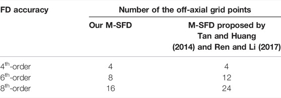
TABLE 1. Number of the off-axial grid points required by our M-SFD and the previous M-SFD to make the FD discrete acoustic wave equation reach specified order accuracy.

3 Elastic Wave Modeling Strategy With High Accuracy

For elastic wave simulation with M-SFD, the FD coefficients calculated with P- or S-wave time–space domain dispersion relation can only ensure the P- or S-wave to achieve high modeling accuracy respectively. In order to improve the modeling accuracy of P- and S-wave simultaneously, the elastic wave Equation 5 can be decomposed as (Li et al., 2007)

$\begin{array}{cc}{\upsilon }_x={\upsilon }_x^P+{\upsilon }_x^S,& {\upsilon }_z={\upsilon }_z^P+{\upsilon }_z^S\end{array},(24)$

$\begin{array}{l}\begin{array}{cc}\frac{\partial {\upsilon }_x^P}{\partial t}=\frac{1}{\rho }\frac{\partial {\tau }_{xx}^P}{\partial x},& \frac{\partial {\upsilon }_z^P}{\partial t}=\frac{1}{\rho }\frac{\partial {\tau }_{zz}^P}{\partial z},\end{array}\\ \begin{array}{cc}\frac{\partial {\tau }_{xx}^P}{\partial t}=\left(\lambda +2\mu \right)\left(\frac{\partial {\upsilon }_x}{\partial x}+\frac{\partial {\upsilon }_z}{\partial z}\right),& \frac{\partial {\tau }_{zz}^P}{\partial t}=\left(\lambda +2\mu \right)\left(\frac{\partial {\upsilon }_x}{\partial x}+\frac{\partial {\upsilon }_z}{\partial z}\right)\end{array},\end{array}(25)$

$\begin{array}{l}\begin{array}{cc}\frac{\partial {\upsilon }_x^S}{\partial t}=\frac{1}{\rho }\left(\frac{\partial {\tau }_{xx}^S}{\partial x}+\frac{\partial {\tau }_{xz}^S}{\partial z}\right),& \frac{\partial {\upsilon }_z^S}{\partial t}=\frac{1}{\rho }\left(\frac{\partial {\tau }_{xz}^S}{\partial x}+\frac{\partial {\tau }_{zz}^S}{\partial z}\right)\end{array},\\ \begin{array}{ccc}\frac{\partial {\tau }_{xx}^S}{\partial t}=-2\mu \frac{\partial {\upsilon }_z}{\partial z},& \frac{\partial {\tau }_{zz}^S}{\partial t}=-2\mu \frac{\partial {\upsilon }_x}{\partial x},& \frac{\partial {\tau }_{xz}^S}{\partial t}=\mu \left(\frac{\partial {\upsilon }_x}{\partial z}+\frac{\partial {\upsilon }_z}{\partial x}\right)\end{array}.\end{array}(26)$

The workflow to solve the decomposed elastic wave equations with M-SFD is as follows: ① the FD discrete equations for the decomposed P-wave (equation 25) and S-wave (Equation 26) with M-SFD are derived. ② The discrete P-wave equation is solved with the FD coefficients computed by the P-wave time-space domain dispersion relation. ③ The discrete S-wave equation is solved with FD coefficients computed by the S-wave time-space domain dispersion relation. ④ ${\upsilon }_x$ and ${\upsilon }_z$ are updated at the current moment using Eq. 24. ⑤ Steps ②-④ are repeated until the maximum recording time is reached.

According to the aforementioned workflow, the decomposed P- and S-wave equations are solved with the FD coefficients calculated based on the P- and S-wave time-space domain dispersion relation respectively, and then P- and S-wave can reach high modeling accuracy at the same time.

4 Dispersion and Stability Analyses

4.1 Dispersion Analysis

According to Eq. 9 and the phase velocity formula $v_{ph}=\omega /k$, we define an error function ${\epsilon }_{ph}\left(\theta \right)$ of normalized phase velocity to describe numerical dispersion for M-SFD (N=1), and ${\epsilon }_{ph}\left(\theta \right)$ is given by

$\begin{array}{c}{\epsilon }_{ph}\left(\theta \right)=\frac{v_{ph}}{v}-1=\frac{2}{rkh}{\sin }^{-1}\left(r\sqrt{q}\right)-1,\\ q={\left\{{\displaystyle \sum _{m=1}^M{a}_m\sin \left[\left(m-1/2\right)kh\cos \theta \right]}+2b_1\cos \left(kh\sin \theta \right)\sin \left(\frac{kh\cos \theta }{2}\right)\right\}}^2\\ +{\left\{{\displaystyle \sum _{m=1}^M{a}_m\sin \left[\left(m-1/2\right)kh\sin \theta \right]}+2b_1\cos \left(kh\cos \theta \right)\sin \left(\frac{kh\sin \theta }{2}\right)\right\}}^2.\end{array}(27)$

If ${\epsilon }_{ph}\left(\theta \right)$ equals 1, there is no dispersion, if ${\epsilon }_{ph}\left(\theta \right)$ is smaller than 1, space dispersion will occur, and if ${\epsilon }_{ph}\left(\theta \right)$ is larger than 1, time dispersion will occur.

Similarly, we can derive the expressions of ${\epsilon }_{ph}\left(\theta \right)$ for M-SFD (N=2, 3, and 4). Furthermore, according to the P- and S-wave time-space domain dispersion relation, the expressions of ${\epsilon }_{ph}\left(\theta \right)$ for P- and S-wave can be derived.

Using the expressions of ${\epsilon }_{ph}\left(\theta \right)$, we can plot the phase velocity dispersion curves of C-SFD and M-SFD (N=1, 2, 3, and 4) and then analyze the numerical dispersion characteristics.

Figure 3 gives the phase velocity dispersion curves of C-SFD (M=2, 5, 8) and M-SFD (M=2, 5, and 8; N=1) with $r=0.3$ for acoustic wave simulation. This figure shows several important phenomena: i) Both C-SFD (M=2) and M-SFD (M=2; N=1) have obvious space dispersion. ii) C-SFD (M=5,8) shows obvious time dispersion, and the dispersion does not decrease as M increases from 5 to 8. iii) The dispersion curves of M-SFD (M=5,8) converge well, and the dispersion decreases further as M increasing from 5 to 8. Based on the analyses we can infer that when M is small (M is about 2), both M-SFD and C-SFD cannot suppress the numerical dispersion well, and when M is large (M is about 8) M-SFD can suppress the numerical dispersion more effectively than C-SFD, to gain higher accuracy for acoustic wave modeling.

FIGURE 3

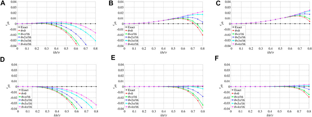
FIGURE 3. Phase velocity dispersion curves of the acoustic staggered-grid FD schemes with $r=0.3$. (A–C) C-SFD (M=2, 5, and 8); (D–F) M-SFD (M=2, 5, and 8; N=1).

Figure 4 gives the phase velocity dispersion curves of M-SFD (M=6, 18, 30; N=1, 2, 3, and 4) with $r=0.3$. This figure involves three columns (A-D), (E-H), and (I-L); each column has its own scale on the vertical axis. From this figure, there are some points that deserve to be mentioned: i) When M is 6, the differences in the numerical dispersion of M-SFD (N=1,2,3,4) are negligible. ii) When M is 18, the dispersion curves of M-SFD are of better convergence and display lower numerical dispersion when N varies from one to two; nonetheless, the dispersion characteristics of M-SFD have a high similarity even if N has been increased to four after then. iii) When M is 30, the dispersion curves of M-SFD are of better convergence as N varies from one to two, and further increasing N up to four, the dispersion curves will exhibit much better convergence and even lower numerical dispersion.

FIGURE 4

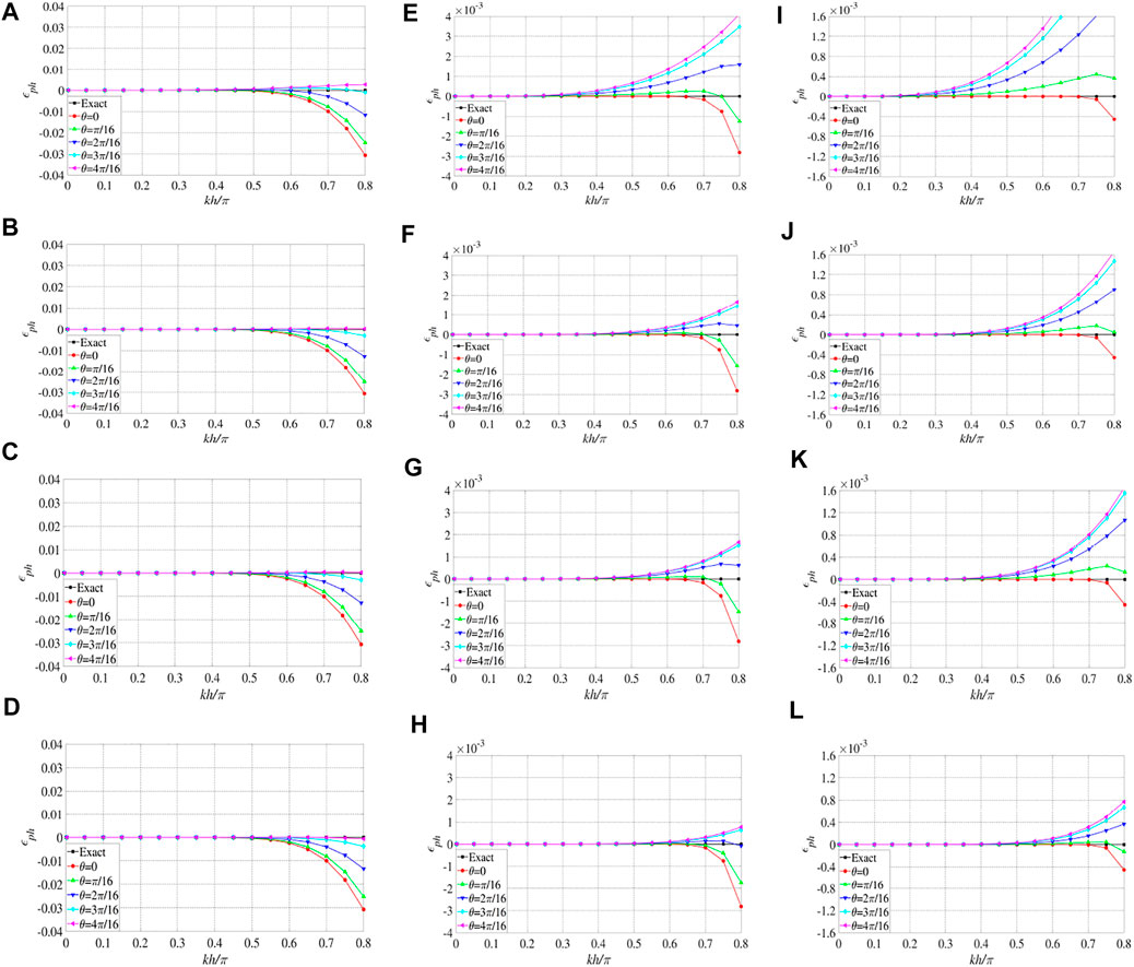
FIGURE 4. Phase velocity dispersion curves of the acoustic staggered-grid FD schemes with $r=0.3$. (A–D) M-SFD (M=6; N=1, 2, 3, and 4), (E–H) M-SFD (M=18; N=1, 2, 3, and 4), (I–L) M-SFD (M=30; N=1, 2, 3, and 4).

From the aforementioned analyses, we can infer that, for acoustic wave simulation with M-SFD, the modeling accuracy is relatively high for general usage with N=1 and M being about 6, and the modeling accuracy can meet extremely strict conditions with N=2 and M being about 18. The modeling accuracy further improves with N=4 and M being about 30, but it is not recommended due to very low efficiency. So wave equation modeling with M-SFD can balance modeling accuracy and efficiency by taking proper values for N and M.

We can also find in Figure 4 that, increasing N from 2 to 3 while M is fixed, the dispersion characteristics of M-SFD are unchanged. This is due to the fact that the FD discrete acoustic wave equations given by M-SFD (N=2,3) are both sixth-order accuracy.

Figure 5 displays the P-wave and S-wave phase velocity dispersion curves of C-SFD (M=8) and M-SFD (M=8; N=1) with $r_p=0.45$ and $r_s=0.25$. The dispersion curves of M-SFD (M=8;N=1) are plotted with the FD coefficients calculated with different methods. From this figure, four conclusions can be deduced: i) For C-SFD (M=8), both the P-wave and S-wave have obvious time dispersion. ii) For M-SFD (M=8;N=1), with FD coefficients calculated based on P-wave time-space domain dispersion relation, P-wave shows small dispersion but S-wave shows obvious space dispersion, and with FD coefficients calculated based on S-wave time-space domain dispersion relation, S-wave shows small dispersion but P-wave shows obvious time dispersion. iii) For M-SFD (M=8;N=1), with the FD coefficients calculated based on the P- and S-wave time-space domain dispersion relation respectively, the dispersion of both P- and S-wave is small, i.e., solving the decomposed P- and S-wave equation with the FD coefficients calculated based on the P- and S-wave time-space domain dispersion relation respectively can ensure both P- and S-wave to reach high modeling accuracy. iv) Comparing Figures 5A, C, the numerical dispersion of both P-wave and S-wave of M-SFD (M=8;N=1) is smaller than that of C-SFD (M=8), when the FD coefficients of M-SFD (M=8;N=1) are calculated based on the S-wave time-space domain dispersion relation.

FIGURE 5

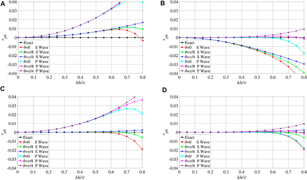
FIGURE 5. P-wave and S-wave phase velocity dispersion curves of the elastic staggered-grid FD schemes with $r_p=0.45$ and $r_s=0.25$. (A) C-SFD (M=8) and (B) M-SFD (M=8; N=1) with the FD coefficients calculated based on the P-wave time–space domain dispersion relation. (C) M-SFD (M=8; N=1) with the FD coefficients calculated based on the S-wave time–space domain dispersion relation. (D) M-SFD (M=8; N=1), the P-wave, and S-wave phase velocity dispersion curves are plotted with the FD coefficients calculated based on the P-wave and S-wave time–space domain relation, respectively.

4.2 Stability Analysis

According to Eq. 9, we can get

$\begin{array}{c}\frac{1}{r^2}\sin \left(\frac{rkh}{2}\right)\approx {\left\{{\displaystyle \sum _{m=1}^M{a}_m\sin \left[\left(m-1/2\right)k_{x}h\right]}+2b_1\cos \left(k_{z}h\right)\sin \left(\frac{k_{x}h}{2}\right)\right\}}^2\\ +{\left\{{\displaystyle \sum _{m=1}^M{a}_m\sin \left[\left(m-1/2\right)k_{z}h\right]}+2b_1\cos \left(k_{x}h\right)\sin \left(\frac{k_{z}h}{2}\right)\right\}}^2.\end{array}(28)$

Letting $k_x=k_z=\pi /h$ and considering $0\le {\sin }^2\left(rkh/2\right)\le 1$, we have

$r\le S=\frac{1}{\sqrt{2}\left|{\displaystyle \sum _{m=1}^M{\left(-1\right)}^{m-1}{a}_m}-2b_1\right|},(29)$

where $S$ is the stability factor.

Equation 29 represents the stability condition of the FD discrete acoustic wave equation given by M-SFD (N=1). Similarly, the stability condition of C-SFD and M-SFD (N=2,3,4) can also be derived. Furthermore, we can also derive the P-wave and S-wave stability conditions of C-SFD and M-SFD (N=1,2,3,4) in the same way.

Figure 6 displays the curve of maximum $r$ limited by the stability condition with M, which is called the stability curve. Figure 6A shows the stability curves of the FD discrete acoustic wave equation given by C-SFD and M-SFD (N=1,2,3,4). In most cases $r_p>r_s$, so the stability of the FD discrete elastic wave equation is determined by the P-wave stability. If the FD coefficients are calculated based on the P-wave time-space domain dispersion relation for M-SFD (N=1,2,3,4), the P-wave stability curves of C-SFD and M-SFD (N=1,2,3,4) are identical to Figure 6A. With the FD coefficients calculated based on the S-wave time-space domain dispersion relation for M-SFD (N=1,2,3,4), the P-wave stability curves of C-SFD and M-SFD (N=1,2,3,4) are shown in Figure 6B.

FIGURE 6

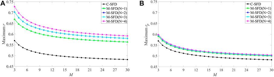
FIGURE 6. Stability curves of the FD discrete (A) acoustic wave and (B) elastic wave equation given by C-SFD and M-SFD (N=1, 2, 3, and 4). In (B), the FD coefficients are calculated with the S-wave time–space domain dispersion relation for M-SFD (N=1, 2, 3, and 4).

Figure 6 demonstrates that for acoustic and elastic wave simulation, the stability of M-SFD (N=1,2,3,4) is better than C-SFD. In addition, the stability of M-SFD with N=2 and N=3 is identical. This can be explained by the same order accuracy of the FD discrete wave equations given by M-SFD (N=2,3).

5 Numerical Modeling and RTM

5.1 Acoustic Wave Modeling

A three-layer model is designed to test our M-SFD method. The horizontal and vertical grid numbers of the model are both 601, with grid size equaling 15 m. The depths of the two reflecting interfaces are 3000 and 4950m, respectively. The acoustic velocities of the three layers are 2400, 2700, and 3200 m/s, respectively. A Ricker wavelet source with a dominant frequency of 20 Hz is located at (750 m, 750 m). Acoustic simulations are performed with C-SFD (M=10) and M-SFD (M=8; N=1), with time step $\mathit{\Delta }t=1.0\text{ms}$ and $\mathit{\Delta }t=1.5\text{ms}$, respectively. Figure 7 shows the modeling snapshots at 3.0 s.

FIGURE 7

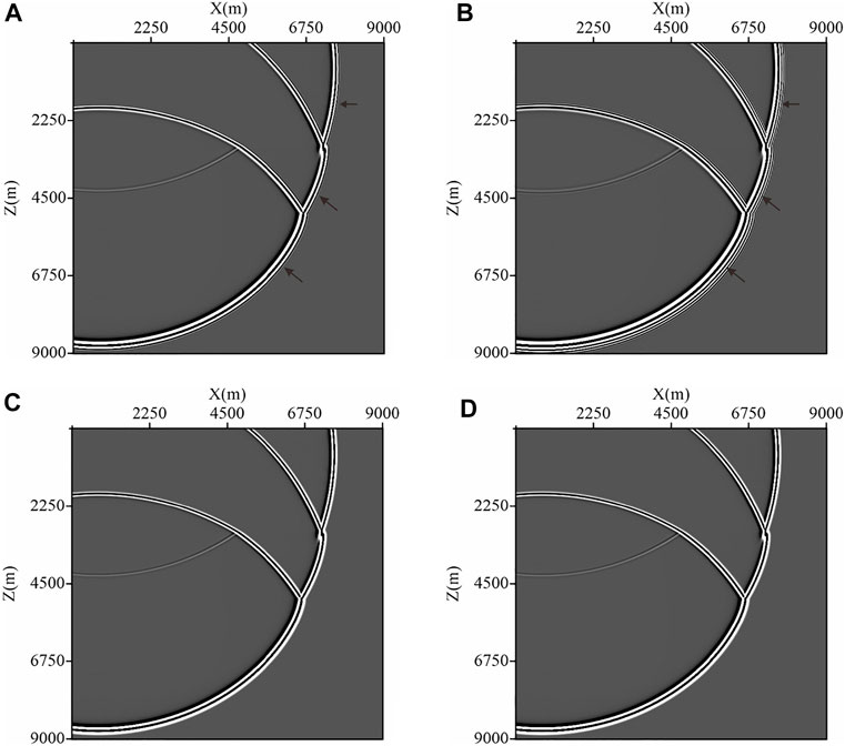
FIGURE 7. Acoustic snapshots at 3.0s for the three-layered model. (A,B) C-SFD (M=10) with the time step $\mathit{\Delta }t=1.0\text{ms}$ and $\mathit{\Delta }t=1.5\text{ms}$. (C) (D) M-SFD (M=8; N=1) with time step $\mathit{\Delta }t=1.0\text{ms}$ and $\mathit{\Delta }t=1.5\text{ms}$.

A complex structure model representative of the Tarim Basin in Western China is shown in Figure 8A. The horizontal and vertical grid numbers of the model are 1,201 and 526 respectively, with grid size equaling 15 m. A Ricker wavelet with a dominant frequency of 25 Hz is used as the source, located at (9000 m, 150 m). Acoustic numerical simulations are conducted with C-SFD (M=10) and M-SFD (M=8; N=1), with time step $\mathit{\Delta }t=1.0\text{ms}$ and $\mathit{\Delta }t=1.5\text{ms}$ respectively. Figure 8B shows a seismic record modeled by M-SFD (M=8; N=1) with $\mathit{\Delta }t=1.5\text{ms}$. Figures 8C–F give the amplified local parts of the seismic records modeled by C-SFD (M=10) and M-SFD (M=8; N=1) with $\mathit{\Delta }t=1.0\text{ms}$ and $\mathit{\Delta }t=1.5\text{ms}$.

FIGURE 8

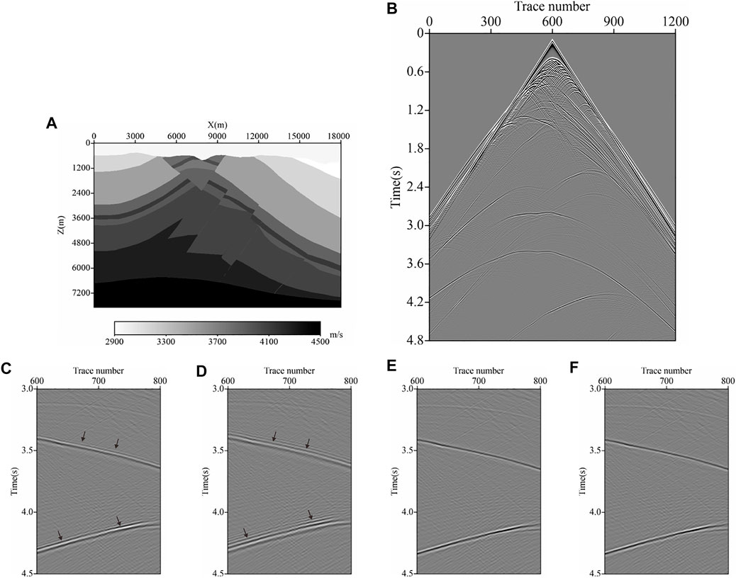
FIGURE 8. (A) Typical complex structural model of the Tarim Basin in Western China; (B) acoustic record modeled by M-SFD (M=8; N=1) with time step $\mathit{\Delta }t=1.5\text{ms}$; (C) (D) local parts of the acoustic record modeled by C-SFD (M=10) with $\mathit{\Delta }t=1.0\text{ms}$ and $\mathit{\Delta }t=1.5\text{ms}$; (E,F) local parts of the acoustic record modeled by M-SFD (M=8; N=1) with $\mathit{\Delta }t=1.0\text{ms}$ and $\mathit{\Delta }t=1.5\text{ms}$.

The spatial FD operators of C-SFD (M=10) and M-SFD (M=8; N=1) are both composed of 20 grid points, so the computational amount of one iteration for C-SFD (M=10) and M-SFD (M=8; N=1) is almost the same. Then, C-SFD (M=10) and M-SFD (M=8; N=1) will be almost the same computational efficiency when the same time step is adopted.

Comparing the snapshots in Figure 7 and the amplified regions of the seismic records in Figures 8C–F, we find that slight time dispersion exists in the results simulated by C-SFD (M=10) with time step $\mathit{\Delta }t=1.0\text{ms}$. As the time step increasing to $\mathit{\Delta }t=1.5\text{ms}$, the time dispersion becomes more serious. However, there is no obvious dispersion in the results modeled by M-SFD (M=8; N=1) with time step $\mathit{\Delta }t=1.0\text{ms}$ and $\mathit{\Delta }t=1.5\text{ms}$. Therefore, M-SFD (M=8; N=1) can suppress the numerical dispersion better than C-SFD (M=10), when the same time step is adopted. That is to say, with almost the same computational efficiency, M-SFD (M=8; N=1) can reach higher modeling accuracy than C-SFD (M=10). Furthermore, we find that M-SFD (M=8; N=1) with $\mathit{\Delta }t=1.5\text{ms}$ can suppress the numerical dispersion better than C-SFD (M=10) with $\mathit{\Delta }t=1.0\text{ms}$, so compared to C-SFD (M=10), M-SFD (M=8; N=1) can take larger time step to reach higher computational efficiency and get higher modeling accuracy at the same time.

5.2 Elastic Wave Modeling

The first elastic wave modeling is carried out on a three-layered model. The horizontal and vertical grid numbers of the model are both 601, with grid size equaling 10 m. The P-wave velocities of the three layers are 2400, 2700, and 3200 m/s, and the S-wave velocities of the three layers are 1500, 1620, and 1800 m/s respectively. The depths of the two reflectors are 2000 and 3300 m. A Ricker wavelet source with a dominant frequency of 20 Hz is located at (500 m, 500 m). Figures 9, 10 show the snapshots of the ${\upsilon }_x$ and ${\upsilon }_z$ component at 2.4 s modeled by C-SFD (M=10) and M-SFD (M=8; N=1) with $\mathit{\Delta }t=1.5\text{ms}$.

FIGURE 9

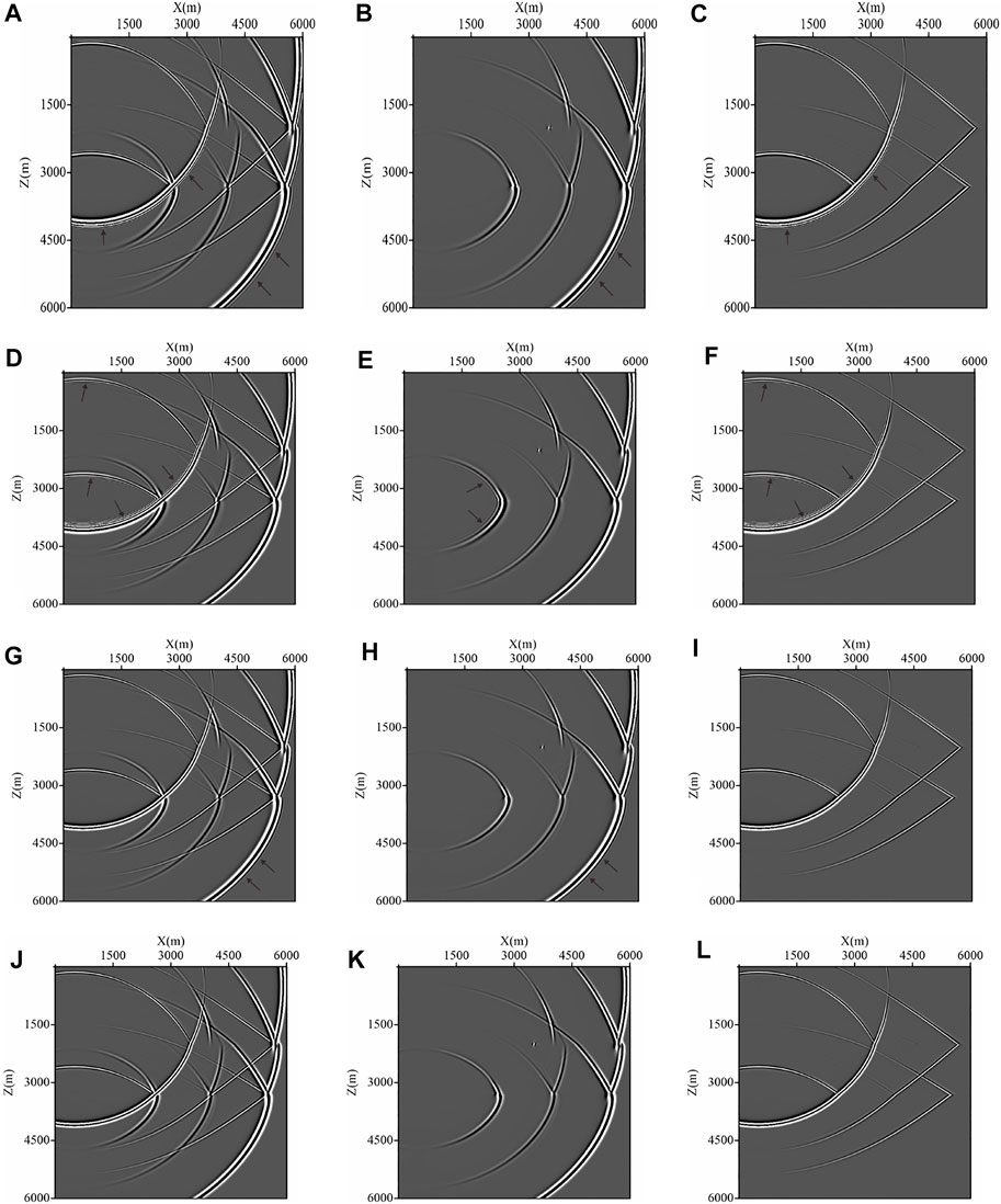
FIGURE 9. Elastic snapshots of ${\upsilon }_x$ and decomposed P- and S-wave components at 2.4 s for the three-layered model simulated with time step $\mathit{\Delta }t=1.5\text{ms}$. (A–C) C-SFD (M=10), (D–F), and (G–I) M-SFD (M=8; N=1) with the FD coefficients calculated based on the P- and S-wave time-space domain dispersion relation, respectively. (J–L) M-SFD (M=8; N=1), solving the decomposed P- and S-wave equations.

FIGURE 10

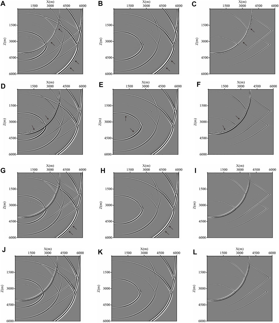
FIGURE 10. Elastic snapshots of ${\upsilon }_z$ and decomposed P- and S-wave components at 2.4 s for the three-layered model simulated with time step $\mathit{\Delta }t=1.5\text{ms}$. (A–C) C-SFD (M=10), (D–F), and (G–I) M-SFD (M=8; N=1) with the FD coefficients calculated based on the P- and S-wave time-space domain dispersion relation, respectively. (J–L) M-SFD (M=8; N=1), solving the decomposed P- and S-wave equations.

Figures 9, 10 indicate that in the result modeled by C-SFD (M=10), both P-wave and S-wave show obvious time dispersion. In the result modeled by M-SFD (M=8; N=1) with the FD coefficients calculated based on the P-wave time-space domain dispersion relation, P-wave has no obvious numerical dispersion, but obvious space dispersion exists in S-wave. In the result modeled by M-SFD (M=8; N=1) with the FD coefficients calculated based on the S-wave time-space domain dispersion relation, S-wave has no obvious numerical dispersion, but slight time dispersion exists in P-wave. In the result modeled by M-SFD (M=8; N=1) with the decomposed P- and S-wave equation, both P- and S-wave have no obvious numerical dispersion.

Based on the aforementioned analyses, we can infer that with almost the same computational efficiency, M-SFD (M=8; N=1), with the FD coefficients calculated based on the S-wave time-space domain dispersion relation, suppresses the numerical dispersion of both P- and S-wave more effectively to obtain higher modeling accuracy than C-SFD (M=10). In addition, solving the decomposed P- and S-wave equations with M-SFD (M=8; N=1) can further improve the modeling accuracy. But it will increase the amount of computation and the occupation of memory. Calculating The FD coefficients based on the P-wave time-space domain dispersion relation for M-SFD (M=8; N=1) is not recommended, which causes serious spatial dispersion for S-wave.

The typical complex structural model of the Tarim Basin of Western China is used in the following simulation. The P-wave velocity model is shown in Figure 8A. The S-wave velocity is generated by dividing 1.8 by the P-wave velocity. The grid size is changed to 10 m. A Ricker wavelet with a dominant frequency of 20 Hz is used as the source, located at (6000 m, 100 m). Figure 11A–D display the amplified regions of the seismic records of the ${\upsilon }_z$ component modeled by C-SFD (M=10) and M-SFD (M=8; N=1) with time step $\mathit{\Delta }t=1.0\text{ms}$.

FIGURE 11

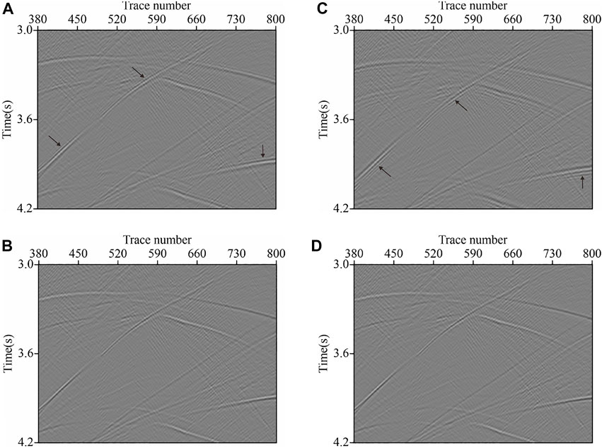
FIGURE 11. Local parts of the elastic record of the ${\upsilon }_z$ component for the complex structural model simulated with time step $\mathit{\Delta }t=1.0\text{ms}$: (A) C-SFD (M=10); (B,C) M-SFD (M=8; N=1) with the FD coefficients calculated based on the P-wave and S-wave time-space domain dispersion relation, respectively; (D) M-SFD (M=8; N=1), solving the decomposed P-wave and S-wave equation.

By examining the zoomed region of the seismic records we can see that the seismic record modeled by C-SFD (M=10) shows obvious time dispersion. With the FD coefficients calculated based on the P-wave time-space domain dispersion relation, the seismic record modeled by M-SFD (M=8; N=1) shows some space dispersion. With the FD coefficients calculated based on the S-wave time-space domain dispersion relation, the seismic record modeled by M-SFD (M=10; N=1) displays no obvious dispersion. The seismic record obtained by solving the decomposed P-wave and S-wave equation with M-SFD (M=10; N=1) also has no obvious dispersion, but it is of high computational expense and memory occupation.

The aforementioned analyses demonstrate that for elastic wave simulation, with almost the same computational efficiency, M-SFD (M=8; N=1), with the FD coefficients calculated based on the S-wave time-space domain dispersion relation, can suppress the numerical dispersion more effectively to reach higher modeling accuracy than C-SFD (M=10).

5.3 Acoustic RTM

We further extend M-SFD to acoustic wave RTM and then perform an RTM test on the complex structure model in Figure 8A. The source wavelet is a Ricker wavelet with a dominant frequency of 25 Hz. And 150 shot gathers without numerical dispersion are modeled by C-SFD (M=15) with a very small time step$\mathit{\Delta }t=0.1\text{ms}$, which is used as the input gathers for RTM. Each shot gathered has 600 traces. The source interval is 120 m and the trace interval is 30 m.

We use C-SFD (M=10) and M-SFD (M=8; N=1) as the wavefield propagation operator of the RTM with the time step $\mathit{\Delta }t=1.5\text{ms}$. The cross-correlation imaging condition is adopted and the Laplace filter is used to suppress the low-frequency noise that existed in the RTM results. Figure 12 shows the final RTM result with C-SFD (M=10) and M-SFD (M=8; N=1) respectively. It exhibits that, there are serious imaging artifacts caused by the numerical dispersion in the deep portion of the RTM result with C-SFD (M=10). While the imaging artifacts are successfully suppressed in the RTM result with M-SFD (M=8; N=1). So M-SFD used as the wavefield propagation operator in RTM can improve the imaging accuracy and resolution of deep structures.

FIGURE 12

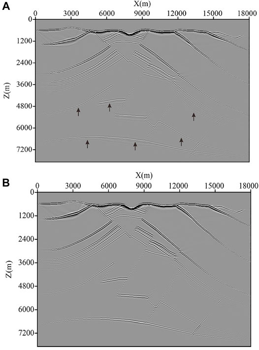
FIGURE 12. Acoustic wave RTM results with (A) C-SFD (M=10) and (B) M-SFD (M=8; N=1) for the typical complex structural model of the Tarim Basin in Western China.

6 Discussion

In this section, we discussed the stability of C-SFD and M-SFD for elastic wave simulation on a medium with a high Poisson’s ratio. A two-layered model shown in Figure 13 is adopted, with a grid size equaling 10 m. The Poisson’s ratios of the layer are 0.395 and 0.306. Figure 13(B-E) displays the snapshots of the ${\upsilon }_z$ component at 1.8 s simulated by C-SFD (M=10) and M-SFD (M=8; N=1).

FIGURE 13

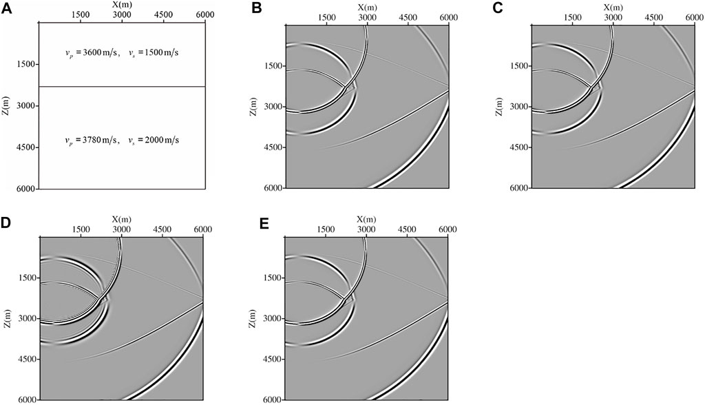
FIGURE 13. Layered model and snapshots of the ${\upsilon }_z$ component simulated by different SFD schemes. (A) Two-layered model. (B) C-SFD (M=10) with $\mathit{\Delta }t=1\text{ms}$. (C) M-SFD (M=8; N=1) with $\mathit{\Delta }t=1\text{ms}$, the FD coefficients calculated based on the P-wave time-space domain dispersion relation. (D) M-SFD (M=8; N=1) with $\mathit{\Delta }t=1.5\text{ms}$, the FD coefficients calculated based on the S-wave time-space domain dispersion relation. (E) M-SFD (M=8; N=1) with $\mathit{\Delta }t=1.5\text{ms}$, solving the decomposed P-wave and S-wave equations.

Limited to the stability condition, the simulation by C-SFD (M=10), with a time step $\mathit{\Delta }t$ equaling 1.0 ms, is stable, while $\mathit{\Delta }t$ increasing to 1.5 ms, it becomes unstable. Similarly, with the FD coefficients calculated based on the S-wave time-space domain dispersion relation, the simulation by M-SFD (M=8; N=1) is stable with $\mathit{\Delta }t=1.0\text{ms}$ but unstable with $\mathit{\Delta }t=1.5\text{ms}$. With the FD coefficients calculated based on the P-wave time-space domain dispersion relation, the simulation by M-SFD (M=8; N=1) is stable with $\mathit{\Delta }t=1.5\text{ms}$, but obvious space dispersion exists in the modeling snapshot. Solving the decomposed P- and S-wave equations by M-SFD (M=8; N=1) with $\mathit{\Delta }t=1.5\text{ms}$ is also stable.

The aforementioned analyses show that both C-SFD and M-SFD are suitable for elastic wave simulation on a model with a high Poisson’s ratio. However, the stability of M-SFD is better than C-SFD, when the FD coefficients are calculated based on the P-wave time-space domain dispersion for M-SFD or the simulation is implemented by solving the decomposed P- and S-wave equations with M-SFD. The better stability ensures M-SFD to adopt a larger time step.

After the comprehensive considerations of the modeling accuracy and stability, elastic wave simulation with M-SFD by solving the decomposed P- and S-wave equations could be a feasible option. Nevertheless, this scheme is at the expense of rather high computational resources, so its superiority of it should be further evaluated thoroughly.

7 Conclusion

In this article, by constructing the spatial FD operator with the axial and off-axial grid points jointly to approximate the first-order spatial derivatives, we developed an M-SFD for acoustic and elastic wave equation simulation. Furthermore, we successfully derived the analytical expression of the FD coefficients based on the time-space domain dispersion relation and TE. Then, FD accuracy analysis, dispersion analysis, stability analysis, numerical simulation, and RTM tests are performed. Several conclusions can be deduced:

1) The FD discrete acoustic equation given by C-SFD can only reach the second-order accuracy, while the FD discrete acoustic equation given by M-SFD (N=1, 2, 4) can reach the fourth, sixth, or eighth-order accuracy, and theoretically, it can reach arbitrary even-order accuracy with increasing N continuously.

2) For acoustic wave simulation, compared to C-SFD, M-SFD can suppress the numerical dispersion more effectively to reach higher modeling accuracy with almost the same computational efficiency. Moreover, M-SFD can achieve higher computational efficiency by adopting a larger time step and reach higher modeling accuracy at the same time.

3) The FD coefficients calculated based on P- or S-wave time-space domain dispersion relation can ensure only the P- or S-wave in the FD discrete elastic wave equation given by M-SFD (N=1,2,4) reaches the fourth, sixth, and eighth-order accuracy respectively. Solving the decomposed P- and S-wave equation with M-SFD (N=1, 2, 4) can make P- and S-waves reach the fourth, sixth, and eighth-order accuracy at the same time.

4) For elastic wave simulation, with almost the same efficiency, M-SFD, with its FD coefficients calculated based on the S-wave time-space domain dispersion relation, can suppress both P- and S-wave dispersion more effectively to achieve higher modeling accuracy than C-SFD. By solving the decomposed P- and S-wave equation with M-SFD, the modeling accuracy can be improved further, but the computation efficiency degrades. The FD coefficients calculated based on the P-wave time-space domain dispersion relation should not be adopted for M-SFD, which causes serious spatial dispersion for the S-wave.

5) For both acoustic and elastic wave simulations, M-SFD has better stability than C-SFD.

6) Compared to C-SFD, M-SFD used as the wavefield propagation operator in RTM more effectively eliminates the imaging artifacts caused by the numerical dispersion, which successfully improves the imaging accuracy and resolution of the deep structure.

Data Availability Statement

The raw data supporting the conclusion of this article will be made available by the authors, without undue reservation.

Author Contributions

WL derived the analytical expression of the FD coefficients and performed the numerical modeling. ZH performed the numerical dispersion analysis. XY performed the stability analysis. GP conducted the RTM. ZX plotted some of the Figures. LH conducted the elastic wave modeling.

Funding

This research is supported by the Project of Science and Technology of CNPC under the Grant No. 2021DJ3501.

Conflict of Interest

Author GP was employed by Tarim Oilfield Company, PetroChina.

The remaining authors declare that the research was conducted in the absence of any commercial or financial relationships that could be construed as a potential conflict of interest.

Publisher’s Note

All claims expressed in this article are solely those of the authors and do not necessarily represent those of their affiliated organizations, or those of the publisher, the editors, and the reviewers. Any product that may be evaluated in this article, or claim that may be made by its manufacturer, is not guaranteed or endorsed by the publisher.

Acknowledgments

We would like to thank the editor Dr. Jianping Huang and the two reviewers for their valuable comments and suggestions, which greatly improved the quality of our article. We also thank Dr. Dunshi Wu and Dr. Wei Zhu for their help in revising this English manuscript.

Supplementary Material

The Supplementary Material for this article can be found online at: https://www.frontiersin.org/articles/10.3389/feart.2022.873541/full#supplementary-material

References

Alford, R. M., Kelly, K. R., and Boore, D. M. (1974). Accuracy of Finite‐difference Modeling of the Acoustic Wave Equation. Geophysics 39 (6), 834–842. doi:10.1190/1.1440470

CrossRef Full Text | Google Scholar

Alterman, Z., and Karal, F. C. (1968). Propagation of Elastic Waves in Layered Media by Finite Difference Methods. Bull. Seismol. Soc. Am. 58 (1), 367–398.

Google Scholar

Berkhout, A. J. G. (2014). Review Paper: An Outlook on the Future of Seismic Imaging, Part I: Forward and Reverse Modelling. Geophys. Prospect. 62 (5), 911–930. doi:10.1111/1365-2478.12161

CrossRef Full Text | Google Scholar

Cao, J., and Chen, J.-B. (2018). A Parameter-Modified Method for Implementing Surface Topography in Elastic-Wave Finite-Difference Modeling. Geophysics 83 (6), T313–T332. doi:10.1190/geo2018-0098.1

CrossRef Full Text | Google Scholar

Carcione, J. M. (2015). Wave Fields in Real Media. Oxford: Elsevier.

Google Scholar

Chen, J.-B., Cao, J., and Li, Z. (2021). A Comparative Study on the Stress Image and Adaptive Parameter-Modified Methods for Implementing Free Surface Boundary Conditions in Elastic Wave Numerical Modeling. Geophysics 86 (6), T451–T467. doi:10.1190/geo2020-0418.1

CrossRef Full Text | Google Scholar

Chu, C., and Stoffa, P. L. (2012). Determination of Finite-Difference Weights Using Scaled Binomial Windows. Geophysics 77 (3), W17–W26. doi:10.1190/geo2011-0336.1

CrossRef Full Text | Google Scholar

Dablain, M. A. (1986). The Application of High‐order Differencing to the Scalar Wave Equation. Geophysics 51 (1), 54–66. doi:10.1190/1.1442040

CrossRef Full Text | Google Scholar

Fornberg, B. (1988). Generation of Finite Difference Formulas on Arbitrarily Spaced Grids. Math. Comp. 51, 699–706. doi:10.1090/s0025-5718-1988-0935077-0

CrossRef Full Text | Google Scholar

Geller, R. J., and Takeuchi, N. (1998). Optimally Accurate Second-Order Time-Domain Finite Difference Scheme for the Elastic Equation of Motion: One-Dimensional Case. Geophys. J. Int. 135 (1), 48–62. doi:10.1046/j.1365-246X.1998.00596.x

CrossRef Full Text | Google Scholar

Hu, Z. D., He, Z. H., Liu, W., Wang, Y. C., Han, L. H., Wang, S. J., et al. (2016). Scalar Wave Equation Modeling Using the Mixed-Grid Finite-Difference Method in the Time-Space Domain (In Chinese). Chin. J. Geophys 59 (10), 3829–3846. doi:10.6038/cjg20161027

CrossRef Full Text | Google Scholar

Hu, Z. D., Liu, W., Yong, X. S., Wang, X. W., Han, L. H., and Tian, Y. C. (2021). Mixed-grid Finite-Difference Method for Numerical Simulation of 3D Wave Equation in the Time-Space Domain (In Chinese). Chin. J. Geophys 64 (8), 2809–2828. doi:10.6038/cjg2021O0296

CrossRef Full Text | Google Scholar

Jo, C. H., Shin, C., and Suh, J. H. (1996). An Optimal 9‐point, Finite‐difference, Frequency‐space, 2-D Scalar Wave Extrapolator. Geophysics 61 (2), 529–537. doi:10.1190/1.1443979

CrossRef Full Text | Google Scholar

Li, Z., Zhang, H., Liu, Q., and Han, W. (2007). Numerical Simulation of Elastic Wavefield Separation by Staggering Grid High-Order Finite-Difference Algorithm (In Chinese). Oil Geophys. Prospect. 42 (5), 510–515.

Google Scholar

Liu, Y. (2013). Globally Optimal Finite-Difference Schemes Based on Least Squares. Geophysics 78 (4), T113–T132. doi:10.1190/geo2012-0480.1

CrossRef Full Text | Google Scholar

Liu, Y. (2014). Optimal Staggered-Grid Finite-Difference Schemes Based on Least-Squares for Wave Equation Modelling. Geophys. J. Int. 197 (2), 1033–1047. doi:10.1093/gji/ggu032

CrossRef Full Text | Google Scholar

Liu, Y., and Sen, M. K. (2009). A New Time-Space Domain High-Order Finite-Difference Method for the Acoustic Wave Equation. J. Comput. Phys. 228 (23), 8779–8806. doi:10.1016/j.jcp.2009.08.027

CrossRef Full Text | Google Scholar

Liu, Y., and Sen, M. K. (2011). Scalar Wave Equation Modeling with Time-Space Domain Dispersion-Relation-Based Staggered-Grid Finite-Difference Schemes. Bull. Seismol. Soc. Am. 101 (1), 141–159. doi:10.1785/0120100041

CrossRef Full Text | Google Scholar

Liu, Y., and Sen, M. K. (2013). Time-space Domain Dispersion-Relation-Based Finite-Difference Method with Arbitrary Even-Order Accuracy for the 2D Acoustic Wave Equation. J. Comput. Phys. 232 (1), 327–345. doi:10.1016/j.jcp.2012.08.025

CrossRef Full Text | Google Scholar

Marfurt, K. J. (1984). Accuracy of Finite‐difference and Finite‐element Modeling of the Scalar and Elastic Wave Equations. Geophysics 49 (5), 533–549. doi:10.1190/1.1441689

CrossRef Full Text | Google Scholar

Mittet, R. (2021). On the Pseudospectral Method and Spectral Accuracy. Geophysics 86 (3), T127–T142. doi:10.1190/geo2020-0209.1

CrossRef Full Text | Google Scholar

Moczo, P., Kristek, J., Galis, M., Chaljub, E., and Etienne, V. (2011). 3-D Finite-Difference, Finite-Element, Discontinuous-Galerkin and Spectral-Element Schemes Analysed for Their Accuracy with Respect to P-Wave to S-Wave Speed Ratio. Geophys. J. Int. 187 (3), 1645–1667. doi:10.1111/j.1365-246X.2011.05221.x

CrossRef Full Text | Google Scholar

Moczo, P., Kristek, J., Galis, M., and Pazak, P. (2010). On Accuracy of the Finite-Difference and Finite-Element Schemes with Respect to P-Wave to S-Wave Speed Ratio. Geophys. J. Int. 182 (1), no. doi:10.1111/j.1365-246X.2010.04639.x

CrossRef Full Text | Google Scholar

Mulder, W. A. (2017). A Simple Finite-Difference Scheme for Handling Topography with the Second-Order Wave Equation. Geophysics 82 (3), T111–T120. doi:10.1190/geo2016-0212.1

CrossRef Full Text | Google Scholar

Ren, Z., Dai, X., Bao, Q., Cai, X., and Liu, Y. (2021). Time and Space Dispersion in Finite Difference and its Influence on Reverse Time Migration and Full-Waveform Inversion (In Chinese). Chin. J. Geophys 64 (11), 4166–4180. doi:10.6038/cjg2021P0041

CrossRef Full Text | Google Scholar

Ren, Z., and Li, Z. C. (2017). Temporal High-Order Staggered-Grid Finite-Difference Schemes for Elastic Wave Propagation. Geophysics 82 (5), T207–T224. doi:10.1190/geo2017-0005.1

CrossRef Full Text | Google Scholar

Reshef, M., Kosloff, D., Edwards, M., and Hsiung, C. (1988). Three‐dimensional Elastic Modeling by the Fourier Method. Geophysics 53 (9), 1184–1193. doi:10.1190/1.1442558

CrossRef Full Text | Google Scholar

Pratt, R. G., Shin, C., and Hicks, G. J. (1998). Gauss-Newton and Full Newton Methods in Frequency-Space Seismic Waveform Inversion. Geophys. J. Int. 133 (2), 341–362. doi:10.1046/j.1365-246X.1998.00498.x

CrossRef Full Text | Google Scholar

Shin, C., and Sohn, H. (1998). A Frequency‐space 2-D Scalar Wave Extrapolator Using Extended 25-point Finite‐difference Operator. Geophysics 63 (1), 289–296. doi:10.1190/1.1444323

CrossRef Full Text | Google Scholar

Tan, S., and Huang, L. (2014). An Efficient Finite-Difference Method with High-Order Accuracy in Both Time and Space Domains for Modelling Scalar-Wave Propagation. Geophys. J. Int. 197 (2), 1250–1267. doi:10.1093/gji/ggu077

CrossRef Full Text | Google Scholar

Virieux, J., Calandra, H., and Plessix, R.-É. (2011). A Review of the Spectral, Pseudo-spectral, Finite-Difference and Finite-Element Modelling Techniques for Geophysical Imaging. Geophys. Prospect. 59 (5), 794–813. doi:10.1111/j.1365-2478.2011.00967.x

CrossRef Full Text | Google Scholar

Virieux, J., and Operto, S. (2009). An Overview of Full-Waveform Inversion in Exploration Geophysics. Geophysics 74 (6), WCC1–WCC26. doi:10.1190/1.3238367

CrossRef Full Text | Google Scholar

Wang, E., Liu, Y., and Sen, M. K. (2016). Effective Finite-Difference Modelling Methods with 2-D Acoustic Wave Equation Using a Combination of Cross and Rhombus Stencils. Geophys. J. Int. 206 (3), 1933–1958. doi:10.1093/gji/ggw250

CrossRef Full Text | Google Scholar