The Widening Wealth Inequality as a Contributor to Increasing Household Carbon Emissions

The Sustainable Development Goals call for taking urgent action to combat climate change and reduce inequalities. However, the related actions have not been effective. Global CO2 emissions in 2021 are projected to rebound to approaching the 2018–2019 peak, and wealth inequality has been increasing at the very top of the distribution resulting from the COVID-19 pandemic. To test whether a trade-off exists between social and environmental benefits, this study calculates county-level wealth inequality with the Gini coefficient and consumption-based household carbon emissions with the emissions coefficient method and input–output modeling. Data are collected from the China Family Panel Studies, the Visible Infrared Imaging Radiometer Suite, the Chinese National Bureau of Statistics and Carbon Emission Account and Datasets in 2014, 2016 and 2018. In addition, a high-dimensional fixed-effects model, an instrumental variable model and causal mediation analysis are adopted to empirically test how wealth inequality influences household carbon emissions and explore the underlying mechanisms. The results show that county-level wealth inequality has a positive impact on household carbon emissions per capita. This means that policies designed to narrow the wealth gap can help reduce carbon emissions, making progress toward multiple SDGs. Moreover, the study reveals that the social norms of the Veblen effect and short-termism play an important role in mediating the relationship between wealth inequality and consumption-based household carbon emissions. This finding provides a new perspective to understand the mechanism behind wealth inequality and household carbon emissions related to climate change.

Introduction

Extreme weather events around the world are becoming increasingly frequent, posing a serious threat to the survival of humankind, especially for the poor. Increasing carbon emissions, contributing greatly to global warming and climate change, have therefore become a matter of global concern (IPCC, 2018). The household sector has been one of the largest contributors to carbon emissions due to the direct energy consumption and indirect consumption activities of households (Hertwich and Peters, 2009; Li et al., 2019). Households consume 29% of global energy and are responsible for 21% of the total carbon emissions¹ In the case of China, the largest emitter, the household sector accounts for over 40% of the total carbon emissions and maintains stable growth (Fan et al., 2013; Shi et al., 2016; Shigetomi,2018). 12In May 2020, the Chinese government proposed the domestic-international dual circulation model, which prioritizes domestic consumption to achieve sustainable economic development. The dual circulation plan may further increase the proportion of consumption-based carbon emissions from the household sector.

The increasing significance of consumption-based carbon emissions leads us to rethink the driving factors for household consumption to find effective paths to achieving the carbon-neutral goals outlined in the Paris Agreement (Rogelj et al., 2019). Among the driving factors, the role of inequality, another important SDG and climate action, has also gained great attention from researchers (Piketty and Chancel, 2015; Jorgenson et al., 2017; Rojas-Vallejos and Lastuka, 2020).

Past research has suggested a relationship between income inequality and carbon emissions but failed to achieve consensus (Guo, 2014; Uddin et al., 2020). Ravallion et al. (2000) investigated the relationship between income inequality and carbon emissions from production and proposed that higher inequality comes with less emissions. Sager (2019) further studied the relationship between income inequality and consumption-based carbon emissions using input–output analysis and found that lower income inequality contributes to higher consumption-based carbon emissions. Other researchers insist that income inequality is positively related to carbon emissions (Golley & Meng, 2012; Zhu et al., 2018).

A limitation of these studies is that they have only focused on income inequality and fail to consider the role of wealth inequality. However, wealth is much more concentrated than income because wealth can accumulate over time (Jones, 2015). More importantly, income inequality has declined over the past years, but wealth inequality is worsening following the rapid growth and transformation in China (Wan et al., 2018; Wan et al., 2021). According to the Global Wealth Report in 2021 by Credit Suisse, the Gini coefficient of wealth for China was 0.599 in 2000, rose quickly to 0.636 in 2005 and reached 0.704 in 2020 (see Figure 1). It is therefore imperative to investigate how wealth inequality influences consumption-based carbon emissions.

FIGURE 1

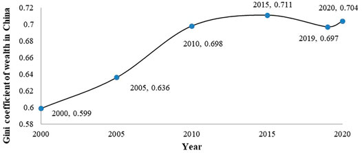
FIGURE 1. Gini coefficient of wealth in China during 2000-2020.

There have been several attempts to study the relationship between wealth inequality and consumption-based carbon emissions. One study, by Knight et al. (2017), reveals that wealth inequality is positively connected with consumption-based carbon emissions in high-income countries. Another study, by Aye (2020), found that wealth inequality has positive effects on carbon emissions. A limitation of these two studies is that they use the top decile of the wealth share to measure wealth inequality. The top decile of the wealth share is easy to calculate but fails to consider the whole wealth distribution. In addition, these studies are limited in that they only use the concentration of political and economic power to explain how wealth inequality influences carbon emissions. However, as some scholars have argued, social norms, including the Veblen effect and short-termism, may also link inequality to consumption-based household carbon emissions, which needs to be verified from the perspective of wealth inequality (Berthe & Elie, 2015; Liobikien, 2020). Moreover, most of the existing studies use mediation analysis to test the mediating mechanism but fail to ensure accurate causal estimation of the relation between the mediator and dependent variable. Mayer et al. (2014) and Kisbu-Sakarya et al.(2020) proposed causal mediation analysis to address this problem.

Against this background, we focus on how wealth inequality influences household carbon emissions and make the following contributions. First, we utilize the Gini coefficient of wealth to measure wealth inequality at the county level. The Gini coefficient can capture variation in the head and tail of the wealth distribution. Moreover, wealth inequality is measured at the county level, while most previous studies focus on the provincial or municipality level. County-level wealth inequality has special links tbo consumer behavior given the similar norms within a county. Besides, as a global problem, carbon emissions decision-making may come from global, national, provincial or municipality strata, but is tangibly implemented at county levels. Therefore, county-level wealth inequality can better reveal the impact of wealth inequality on consumption-based carbon emissions and enrich the limited literature regarding wealth inequality in China. Second, we calculate direct and indirect consumption-based household carbon emissions based on a household survey spanning from 2014 to 2018 in China. This supplements the most recent data on consumption-based carbon emissions in China. Third, we use the instrumental variable method and causal mediation analysis to address the endogeneity problem when evaluating how wealth inequality influences household carbon emissions. Finally, there is no study explaining the influencing mechanism of wealth inequality on consumption-based household carbon emissions based on the role of social norms, including the Veblen effect and short-termism. Our study aims to fill this gap and enriches the literature regarding the specific mechanisms that may link wealth inequality to emissions.

Data and Methods

To determine how wealth inequality influences household carbon emissions, we apply four databases: 1) Samples of China households from the China Family Panel Studies (CFPS) in 2014, 2016 and 2018; 2) The county-level Night Light Development Index (NLDI) from the multitemporal dataset of the Visible Infrared Imaging Radiometer Suite (VIIRS) in 2014, 2016 and 2018; 3) China’s Input–Output Tables (IOTs) in 42 economic sectors from the Chinese National Bureau of Statistics (CNBS) in 2015, 2017 and 2018; and 4) Sectoral emission factor information Carbon Emission Account & Datasets (CEADs) in 2014, 2016 and 2018.

The CFPS and VIIRS: wealth, expenditure, demographics and county features.

The CFPS dataset, launched by Peking University, collects household data on the economic and noneconomic information and wellbeing of the Chinese population at the individual, family, and community levels. It covers 25 provinces/municipalities/autonomous regions in China and does not include Hong Kong, Macao, Taiwan, Xinjiang, Tibet, Qinghai, Inner Mongolia, Ningxia and Hainan (Xie & Lu, 2015). The stratified, three-stage, and probability-proportionate-to-size sampling approach is adopted to improve the randomness and representativeness of the CFPS dataset. First, we feature household wealth by collecting total net assets in the CFPS. Wealth is defined as all household assets minus liabilities, including net housing assets, net financial assets, nonhousing debt, fixed productive assets, land assets, consumer durables and other assets. Second, to calculate indirect household carbon emissions, we collect consumption expenditures in the CFPS. Referring to the classification of household expenditures in the CNBS, consumption expenditures are classified into seven categories of expenditures on food; clothing; residence; household facilities and services; health care and medical services; transportation and telecommunication; and education, culture and recreation.² However, the classification of expenditures in the CFPS does not directly match the 42 economic sectors in the CNBS. To match the two datasets, we disaggregate the consumption expenditure in the CFPS into corresponding sectors in the CNBS, based on the proportion of urban and rural households’ output in 42 economic sectors in IOTs. Third, to measure direct household carbon emissions, we collect expenditures on cooking with fuel, heating with fuel and driving with petrol in the CFPS. Fourth, some scholars assert that conspicuous consumption is the representative case of the Veblen effect. Therefore, referring to Kaus (2013), Berthe & Elie (2015), and Zhou et al. (2018), the Veblen effect is defined as the total household consumption expenditures and proportion of consumption on clothing, residence, transportation and telecommunication to the total expenditure in the CFPS. In addition, the CFPS dataset collects people’s attitudes toward the severity of the environmental problem in China, with scores from 0 to 10. “0” represents “not severe”, while “10” represents “extremely severe”. Echavarren (2017) proposes that people are more likely to emphasize environmental awareness and engage in low-carbon consumption when they perceive the severity of environmental pollution. As those who are short-sighted usually lack environmental awareness and tend to score low for that question (Xu et al., 2017; Xu et al., 2019; Cruz & Manata, 2020), low scores are used to represent the weakening environmental awareness of households caused by short-termism. Fifth, we collect data on household demographic variables, including the child and elderly dependency ratio, proportion of healthy people, log of adult per capita income, access to the internet, and household location. In addition, we capture the characteristic variables of the head of household, such as gender, membership, medicare, age, squared age, marital status and qualifications. Finally, we collect NLDI data in 2014, 2016 and 2018 from the VIIRS to depict county-level economic activities (Chen & Nordhaus, 2015; Wu et al., 2018; Xu et al., 2020; Zhou et al., 2021). These characteristic variables have significant effects on wealth and consumption-based carbon emissions. The definitions of the key variables are displayed in Table 1.

TABLE 1

TABLE 1. Variable definition.

To apply the I-O approach to calculate consumption-based household carbon emissions, we need to integrate household consumption expenditures into IOTs in the CNBS dataset and sectoral carbon emission factors in the CEADs dataset. Given that the CNBS dataset only provides IOTs in 42 economic sectors in 2015, 2017 and 2018, we match IOTs from the CNBS dataset in 2015 and 2017 to corresponding data from the CFPS and CEADs datasets in 2014 and 2016, respectively. Sector classifications are almost the same in the CNBS and CEADs datasets, which greatly reduces the bias due to data matching. With these two datasets, we can calculate the Leontief inverse matrix, which is essential for measuring indirect household carbon emissions and emissions derived from sectoral IOTs and per-yuan carbon emission factors.

Calculation of Wealth Inequality

Following Knight et al. (2017), Liu et al. (2019) and Wan et al. (2021), we adopt the commonly used Gini coefficient to measure wealth inequality at the county level. The Gini coefficient evolves from the Lorenz curve framework and can measure the wealth distribution within a population. It has the benefit of providing an all-inclusive measure of wealth inequality and capturing changes in the head and tail of the wealth spectrum. The Gini coefficient of wealth can be simply expressed as follows:

$\mathit{Gini}=\frac{1}{2{\mathit{n}}^2\mathit{\mu }}{\displaystyle \sum }_{\mathit{h}1=1}^{\mathit{n}}{\displaystyle \sum }_{\mathit{h}2=1}^{\mathit{n}}|\mathit{W}{\mathit{h}}_1-\mathit{W}{\mathit{h}}_2|(1)$

where $Gini$ denotes the county-level Gini coefficient of wealth per adult; $n$ denotes the number of households in the county; and $\mu$ denotes the average per adult household wealth of all households in the county. $W{h}_1$ and $W{h}_2$ represent the per adult wealth of households $h_1$ and $h_2$. Theoretically, $Gini$ ranges from 0 (complete equality) to 1 (complete inequality), which means that the higher $Gini$ is, the greater the wealth inequality is.

Calculation of Direct and Indirect HCEs

As expressed in Eq. 2, the total consumption-based carbon emissions $HCE{s}_{i\_total}$ for households consist of the direct carbon emissions $HCE{s}_{i\_direct}$ and the indirect carbon emissions $HCE{s}_{i\_indirect}$. We use the emissions coefficient method (ECM) from the IPCC (2006) to calculate the direct carbon emissions $HCE{s}_{i\_direct}$ for households and input–output modeling (IOM) to calculate the indirect carbon emissions $HCE{s}_{i\_indirect}$.

$\mathit{HCE}{\mathit{s}}_{\mathit{i}\_\mathit{total}}=\mathit{HCE}{\mathit{s}}_{\mathit{i}\_\mathit{direct}}+\mathit{HCE}{\mathit{s}}_{\mathit{i}\_\mathit{indirect}}(2)$

Emissions Coefficient Method (ECM)

The ECM has been widely used to calculate direct carbon emissions in previous studies (Munksgaard et al., 2000; Wiedenhofer et al., 2017; Zhang, et al., 2020). The direct carbon emissions $HCE{s}_{i\_direct}$ for households are calculated as follows:

$\mathit{HCE}{\mathit{s}}_{\mathit{i}\_\mathit{direct}}={\displaystyle \sum }_{\mathit{j}}{\mathit{f}}_{\mathit{j}}\mathit{Energ}{\mathit{y}}_{\mathit{ji}}(3)$

where $Energ{y}_{ji}$ denotes the energy j consumed by the household and $f_j$ is the carbon emissions factor from energy source j. In the CFPS, there are three main sources of energy consumed by the household: cooking with fuel, heating with fuel and driving with petrol. First, the CFPS dataset classifies cooking fuel into electricity, natural gas, LNG, coal, solar energy and others. Carbon emissions from electricity consumption are usually regarded as indirect HCEs, and emissions from solar energy and others are negligible. Therefore, we calculate energy consumption from cooking fuel based on expenditure and price on natural gas, LNG and coal. Second, given that urban residents in China usually depend on central heating to heat a house, the HCEs of urban households are regarded as indirect carbon emissions, relying on the sector of “Electricity, gas, steam and air conditioning supply”. Because rural residents in China depend on coal for heating, we calculate the energy consumption from heating fuel in rural areas based on the expenditure on heating and the price of coal. Third, local transportation expenses are split into expenditures on public transportation and petrol for self-driving, according to the ratio of urban and rural households’ output in the sectors of “Transportation, Storage, Post and Telecommunication Services” and “Petroleum Processing and Coking” in IOTs. We consider consumption on public transportation as indirect HCEs and calculate the energy consumption from driving petrol from petrol expenditures and prices. We can calculate the direct HCEs by multiplying the direct consumption by the corresponding emissions factors and sum up the results.

Input-Output modeling (IOM)

IOM has also been widely used to calculate the indirect carbon emissions of households (Golley and Meng, 2012; Wiedenhofer et al., 2017), which is similar to the consumer lifestyle approach (CLA). Both IOM and LCA are closely linked to the consumption patterns of the household, while IOM has the unparalleled advantage of systematically covering all the indirect linkages between different industrial sectors. We can use IOM to calculate the indirect carbon emissions $HCE{s}_{i\_indirect}$ as follows:

$\mathit{HCE}{\mathit{s}}_{\mathit{i}\_\mathit{indirect}}=\mathit{D}{(\mathit{I}-\mathit{A})}^{-1}\mathit{Ex}{\mathit{p}}_{\mathit{i}}(4)$

where $D_i$ denotes the row vector of emission factors for sector i. ${(I-A)}^{-1}$, called the Leontief inverse matrix, is essential to the calculation of $HCE{s}_{i\_indirect}$ through the IOM method, where $I$ denotes an identity matrix and $A$ denotes a matrix of direct requirements coefficients. $Ex{p}_i$ is a column vector of expenditure on commodities and services for the household. First, we calculate $D_i$ by $D_i=E_i/V_i$, where $E_i$ denotes the total carbon emissions and $V_i$ denotes the total output for sector i. We can obtain $E_i$ from the CEADs database and $V_i$ from the Chinese National Bureau of Statistics. Second, we multiply $D$ by the Leontief inverse matrix ${(1-A)}^{-1}$ and obtain the total sectoral carbon emission intensity matrix $D{(I-A)}^{-1}$. Third, we multiply the desired expenditure $Ex{p}_i$ by $D{(I-A)}^{-1}$ and obtain the consumption-based indirect carbon emissions by sector. Finally, we classify the sectoral indirect carbon emissions and summarize them by the classification of individual consumption to obtain the indirect carbon emissions for the household. In summary, by applying the CAEDs database, we reduce uncertainty as much as possible. Matching the CEADs database, Chinese National Bureau of Statistics and CFPS database greatly helps us increase the accuracy of the calculation of indirect HCEs (Zhang, et al., 2020).

High-Dimensional Fixed-Effects Model

To evaluate the influence of widening wealth inequality on household carbon emissions, we apply the high-dimensional fixed-effects (HDFE) model. With the HDFE model, it is possible to examine the influence of multiple levels of fixed effects. The household carbon emissions (HCEs) as a function of wealth inequality (WealthInequality) at the county level are represented as follows:

$\mathit{HCE}{\mathit{s}}_{\mathit{i}}={\mathit{\alpha }}_0+{\mathit{\alpha }}_1\mathit{WealthInequalit}{\mathit{y}}_{\mathit{i}}+{\mathit{X}}_{\mathit{i}}\mathit{\beta }+{\mathit{\lambda }}_{\mathit{j}}+{\mathit{\upsilon }}_{\mathit{t}}+{\mathit{\mu }}_{\mathit{i}}(5)$

In this equation, the HDFE model uses control variables ($X_i$) as well as the dependent variable of household carbon emissions and the explanatory variable of wealth inequality. $HCE{s}_i$ denotes consumption-based carbon emissions of the ith household, and $WealthInequalit{y}_i$ denotes the Gini coefficient of wealth in the county where the ith household is located. $X_i$ is a vector of control variables, including features of the household, head of the household and county. Household features refer to the child and elderly dependency ratio, proportion of healthy people, family size, household income per capita, access to the internet and household location. Features of head of the household refer to gender, party, medicare, age, squared age, marital status and qualification. The county feature refers to socioeconomic activities, which is represented by the average nighttime light index at the county level. Region-invariance and time-invariance are captured by the fixed effects, which are ${\lambda }_j$ and ${\upsilon }_t$. Finally, ${\mu }_i$ is the error term.

Instrumental Variable Model

Although we use the HDFE model to improve the robustness of the estimation results, reverse causality and omitted variable bias may occur and cause endogeneity problems. To address such an endogeneity problem, we further use an instrumental variable model (IV) and choose rainfall as an instrumental variable. Rainfall may influence agricultural production and physical assets, especially in rural China. Therefore, rainfall may affect county-level wealth inequality and consumption-based household carbon emissions. Rainfall may not directly influence household carbon emissions, which is an exogenous variable (Yang and Choi, 2007; Akobeng, 2017; Mulubrhan et al., 2018; Zeng et al., 2021). Using the IV, HCEs as a function of wealth inequality can be expressed as:

$\mathit{WealthInequalit}{\mathit{y}}_{\mathit{i}}={\mathit{\alpha }}_0+{\mathit{\alpha }}_2\mathit{Rainfal}{\mathit{l}}_{\mathit{i}}+{\mathit{X}}_{\mathit{i}}\mathit{\beta }+{\mathit{\lambda }}_{\mathit{j}}+{\mathit{\upsilon }}_{\mathit{t}}+{\mathit{\mu }}_{\mathit{i}}(6)$

$\mathit{HCE}{\mathit{s}}_{\mathit{i}}={\mathit{\alpha }}_0+{\mathit{\alpha }}_3\widehat{\mathit{WealthInequalit}{\mathit{y}}_{\mathit{i}}}+{\mathit{X}}_{\mathit{i}}\mathit{\beta }+{\mathit{\lambda }}_{\mathit{j}}+{\mathit{\upsilon }}_{\mathit{t}}+{\mathit{\mu }}_{\mathit{i}}(7)$

where parameter ${\alpha }_3$ is estimated by standard 2SLS estimation. $\widehat{WealthInequalit{y}_i}$ stands for the estimated values of $WealthInequalit{y}_i$ in the first stage. The instrumental variable, $Rainfal{l}_i$, denotes the average annual precipitation in the county where the ith household is located.

Causal Mediation Analysis

To disentangle the mechanisms underlying the association between wealth inequality and household carbon emissions, we need to use mediation analysis. However, typical mediation analysis is essentially a causal model and depends on assumptions that are not consistent with causal conclusions. Therefore, we use mediation analysis (CMA) to improve the accuracy of causal estimation (Mayer et al., 2014; Dippel et al., 2020; Kisbu-Sakarya et al., 2020). The estimation procedure of CMA to identify all linear coefficients is as follows:

1) Under linearity and with the instrument, parameter ${\alpha }_3$ is identified by standard 2SLS estimation, described by Eq. 8 and Eq. 9. $Rainfal{l}_i$ and $WealthInequalit{y}_i$ have the same meanings as above.

$\mathit{WealthInequalit}{\mathit{y}}_{\mathit{i}}={\mathit{\alpha }}_0+{\mathit{\alpha }}_2\mathit{Rainfal}{\mathit{l}}_{\mathit{i}}+{\mathit{X}}_{\mathit{i}}\mathit{\beta }+{\mathit{\lambda }}_{\mathit{j}}+{\mathit{\upsilon }}_{\mathit{t}}+{\mathit{\mu }}_{\mathit{i}}(8)$

$\mathit{Mediato}{\mathit{r}}_{\mathit{i}}={\mathit{\alpha }}_0+{\mathit{\alpha }}_3\widehat{\mathit{WealthInequalit}{\mathit{y}}_{\mathit{i}}}+{\mathit{X}}_{\mathit{i}}\mathit{\beta }+{\mathit{\lambda }}_{\mathit{j}}+{\mathit{\upsilon }}_{\mathit{t}}+{\mathit{\mu }}_{\mathit{i}}(9)$

2) Then, we use $Rainfal{l}_i$ as an instrument for $Mediato{r}_i$, when conditioned on $WealthInequalit{y}_i$, by the following 2SLS model:

$\mathit{Mediato}{\mathit{r}}_{\mathit{i}}={\mathit{\alpha }}_0+{\mathit{\alpha }}_{4\mathit{ra}}\mathit{Rainfal}{\mathit{l}}_{\mathit{i}}+{\mathit{\alpha }}_{4\mathit{wi}}\mathit{WealthInequalit}{\mathit{y}}_{\mathit{i}}+{\mathit{X}}_{\mathit{i}}\mathit{\beta }+{\mathit{\lambda }}_{\mathit{j}}+{\mathit{\upsilon }}_{\mathit{t}}+{\mathit{\mu }}_{\mathit{i}}(10)$

$\mathit{HCE}{\mathit{s}}_{\mathit{i}}={\mathit{\alpha }}_0+{\mathit{\alpha }}_{5\mathit{m}}\widehat{\mathit{Mediato}{\mathit{r}}_{\mathit{i}}}+{\mathit{\alpha }}_{5\mathit{wi}}\mathit{WealthInequalit}{\mathit{y}}_{\mathit{i}}+{\mathit{X}}_{\mathit{i}}\mathit{\beta }+{\mathit{\lambda }}_{\mathit{j}}+{\mathit{\upsilon }}_{\mathit{t}}+{\mathit{\mu }}_{\mathit{i}}(11)$

where parameters ${\alpha }_{5m}$ and ${\alpha }_{5wi}$ are the expected values of the estimators of a 2SLS regression where $WealthInequalit{y}_i$ plays the role of a conditioning variable. $\widehat{Mediato{r}_i}$ is the estimated value of $Mediato{r}_i$ in the first stage.

Results

Descriptive Statistics

Table 2 displays the summary statistics of county-level wealth inequality, household carbon emissions per capita, and control variables. As Table 2 shows, wealth inequality shows an average value of 0.54 and holds steady with the growth of wealth. In addition, we obtain the average total, direct and indirect household carbon emissions per capita in China during 2014-2018 by means of the application of ECM and IOM. The average total household carbon emissions per capita are 2.8 tons. The total direct carbon emissions per capita are 0.28 tons, which is much smaller than the total indirect carbon emissions per capita of 2.52 tons. Table 1 also displays the direct and indirect household carbon emissions per capita across different years. The total, direct and indirect carbon emissions per capita show a stable increment from 2014 to 2018. Most control variables fluctuate slightly throughout the year. Log income per adult in the household increases stably.

TABLE 2

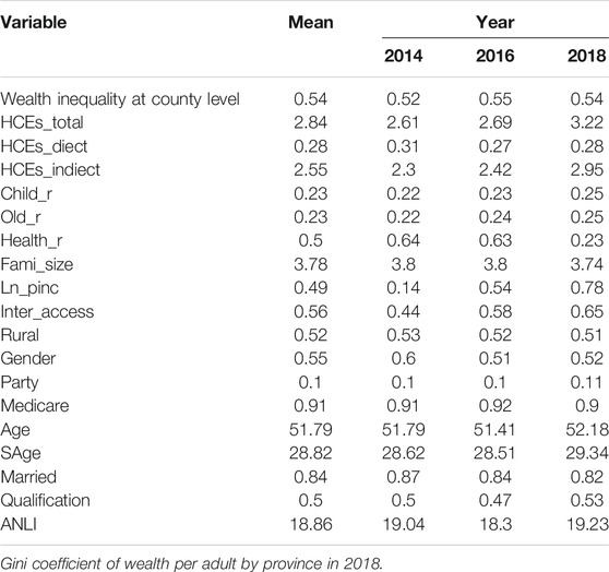
TABLE 2. Description of county-level wealth inequality, household carbon emissions per capital and control variables. Source: Calculated by the authors based on CFPS, IOTs and CEADs in 2014-2018.

Gini Coefficient of Wealth per Adult by Province in 2018

In addition, Figure 2 displays wealth inequality measured by the Gini coefficient of wealth per adult by province in 2018. Both Zhejiang and Heilongjiang obtain relatively low Gini coefficients of wealth per adult, scoring between 0.48 and 0.52 and representing low wealth inequality. The Gini coefficient of Chongqing is much higher, with a score reaching 0.83, followed by Guizhou, Gansu, Hebei, Guangdong, Shandong, Fujian, Sichuan, Jilin and Shaanxi, with scores ranging from 0.62 to 0.7.

FIGURE 2

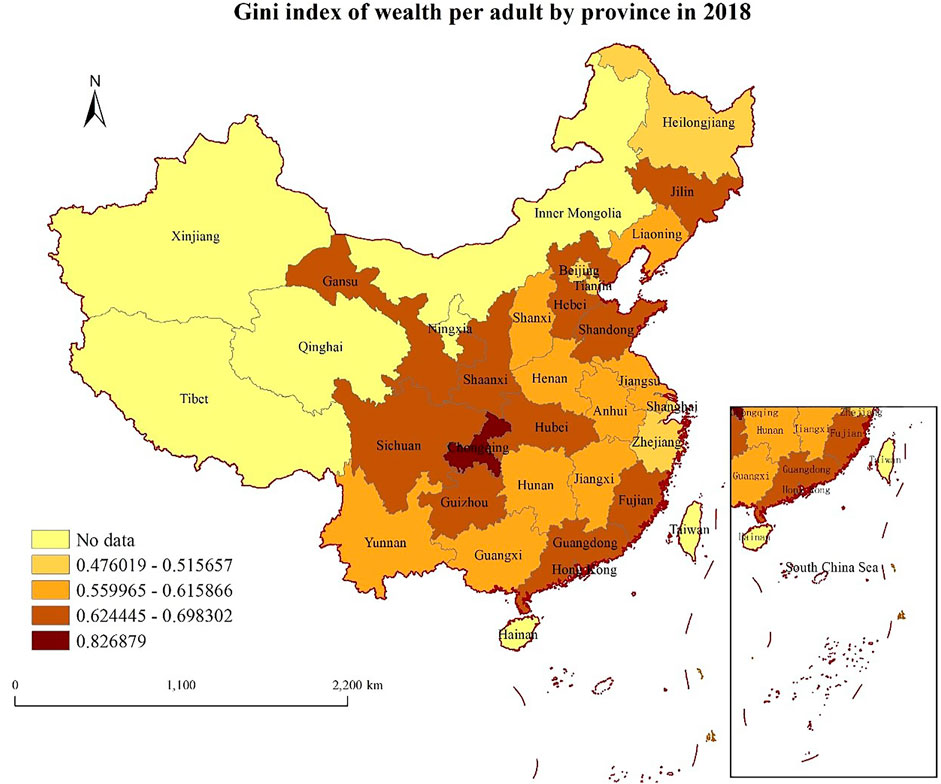
FIGURE 2. Gini coefficient of wealth per adult by province in 2018.

Figure 3 shows the average direct and indirect carbon emissions structure during 2014-2018. We classify the carbon emissions in Table 2 into 7 main categories generated by consumption from food; clothing; residence; household facilities and services; health care and medical services; transportation and telecommunication; and education, culture and recreation. The pie chart shows that indirect carbon emissions per capita account for 90.04%, far more than direct carbon emissions.

FIGURE 3

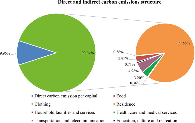
FIGURE 3. Household carbon emissions across wealth percentiles.

Direct and Indirect Carbon Emissions Structure

Figure 4 displays the total, direct and indirect household carbon emissions per capita across different wealth percentiles. Both the direct and indirect carbon emissions per capita first show a slight decrease and then increase with household wealth. These results preliminarily reveal the relationship between household carbon emissions and wealth inequality. However, how wealth inequality influences household carbon emissions needs to be further explored by means of the HDFE and CMA models.

FIGURE 4

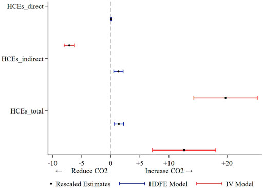
FIGURE 4. The estimated results of regression of the total, direct and indirect household carbon emissions based on HDFE and IV model.

Results of HDFE and IV Models

Table 3 provides the estimated results based on the HDFE and IV models. Columns 1) and 3) in Table 3 display the estimation results without the control variables. To reduce the confounding impact of irrelevant variables, we further control for variables at the individual, family, and county levels in Columns 2) and (4). The estimated results of these two columns show that wealth inequality has a significantly positive effect on total household carbon emissions per capita, with coefficients of 1.384 in the HDFE model and 12.615 in the IV model at the p = 0.01 level. For the control variables, we find a significantly negative correlation between the child and elderly dependency ratio and household carbon emissions per capita in both models. This means that a higher dependency ratio may reduce household carbon emissions per capita. In addition, other variables, including Ln_pinc, Inter_Access, Party, Qualifications and ANLI, have a significantly positive effect on household carbon emissions per capita in both models. These findings indicate that higher income, easier access to the internet, being a CPC member, higher qualifications and faster socioeconomic development may help increase the total carbon emissions per capita of the household.

TABLE 3

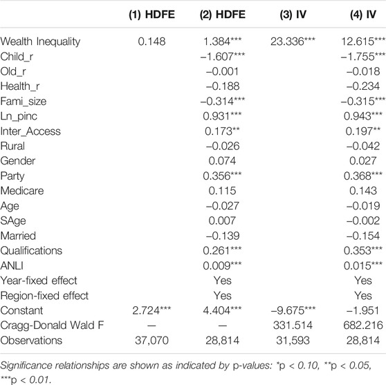
TABLE 3. Estimation results: HDFE and IV regression for HCEs__total during 2014-2018.

To further capture the relationship between wealth inequality and household carbon emissions, we describe the estimated results of the regression of the total, direct and indirect household carbon emissions based on the HDFE and IV models in Figure 4. As it shows, wealth inequality increases household carbon emissions per capita mainly by promoting indirect household carbon emissions. These impacts can be seen in both the HDFE and IV models with significantly positive coefficients. On the other hand, wealth inequality may reduce direct household carbon emissions per capita, with the estimated coefficient being significantly negative in the IV model and insignificantly close to 0 in the HDFE model.

The Role of Social Norms

To study the role of social norms from the perspective of the Veblen effect and short-termism, the IV and CMA models are adopted to test the mediating role of the Veblen effect and short-termism, and the results are displayed in Tables 4, 5, respectively.

TABLE 4

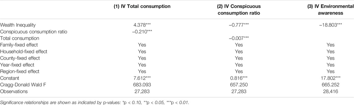
TABLE 4. Estimation results: IV model for mediator.

TABLE 5

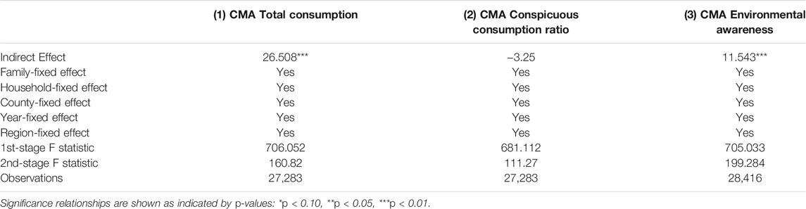
TABLE 5. Estimation results: CMA model for mediator.

Column 1) in Table 4 reveals that wealth inequality can give rise to the growth of total consumption expenditure. Column 1) in Table 5 indicates that the growth of total consumption expenditures that accompanies wealth inequality plays a mediating role in intensifying household carbon emissions per capita. Column 2) in Tables 4, 5 indicates that wealth inequality reduces the conspicuous consumption ratio instead of increasing it. No evidence is found for the role of the conspicuous consumption ratio in wealth inequality increasing household carbon emissions per capita.

As shown in Table 4, Column 3) indicates that the wealth gap can weaken the environmental awareness of households. Column 3) in Table 5 further reveals that greater wealth inequality can increase household carbon emissions per capita by weakening the environmental awareness of households caused by short-termism.

Discussion, Conclusion and Future Research

In this study, we have introduced the Gini coefficient to measure wealth inequality at the county level to display the all-inclusive wealth distribution. The ECM and IOM are used to calculate the direct and indirect HCEs with the most recent large-scale data from the CFPS, CNBS and CEADs spanning 2014 to 2018 in China, making it possible to estimate consumption-based household carbon emissions over time though household-level data. HDFE, IV and CAM are applied to effectively test the impact of wealth inequality on household carbon emissions and the role of social norms of the Veblen effect and short-termism.

The main findings reveal that higher county-level wealth inequality has similar positive influences on household carbon emissions per capita by promoting indirect household carbon emissions as income inequality. The positive impact of income inequality on household carbon emissions has been proven by previous studies (Baek & Gweisah, 2013; Lutz, 2019). This finding is also consistent with the findings of (Knight et al., 2017), who also focuses on wealth inequality. However, (Knight et al., 2016), does not exploit data at the county level and tries to explain the mechanism with political economy theories instead of social norms. Our study aims to fill this gap using a dataset from the CFPS, VIIRS, CNBS and CEADs in 2014, 2016 and 2018.

The second important finding indicates that wealth inequality may increase consumption-based household carbon emissions through the Veblen effect. This finding is consistent with previous studies (Berthe & Elie, 2015; Nielsen et al., 2021). These previous scholars state that consumption is far more than a simple factor of individual utility, but it also plays an important role as social value. Greater wealth inequality in a society means greater differences in social status, therefore causing fierce competition. Such competition is commonly represented by conspicuous consumption, not only in the total consumption level but also in the consumption structure. The middle and lower classes are inspired to copy the consumption patterns of the rich, who tend to overconsume and prefer carbon-intensive products, such as central air conditioning. The Veblen effect highlights the emulative influence of people with high socioeconomic status on increasing household carbon emissions. However, it also offers solutions for reducing household carbon emissions and climate damages if people with high socioeconomic status can assume social responsibilities by reducing unnecessary consumption and consuming low-carbon products.

Another important finding is that wealth inequality has positive effects on consumption-based household carbon emissions by aggravating the short-termism of consumers. This finding also confirms the results of a previous study by Boyce (1994), who proposes that growing wealth inequality may induce short-termism among the rich, middle class and the poor. In such a case, the poor focus on short-term material concerns and are particularly vulnerable to consumerism. They may fail to consider the long-term environmental consequences of their consumption. This means that they may lack environmental awareness and are not inclined to adopt pro-environmental behavior and are prone to carbon-intensive consumption. The rich and middle class may also become trapped in short-termism due to the fear of being caught up with by the lower class in consumption. In this way, wider wealth inequality also raises household carbon emissions through short-termism (Slawinski et al., 2017). This finding highlights the important role of short-termism and adds to a growing body of literature on how wealth inequality influences household carbon consumption.

In addition, this article notes that the total indirect carbon emissions are usually much larger than the direct carbon emissions. In fact, the total indirect carbon emissions are usually much larger than the direct carbon emissions, which is in line with previous studies (Feng et al., 2011; Yang et al., 2017). Compared with previous studies, the calculation results of carbon emissions are similar to the findings of Zhang, et al. (2020), who reported total household carbon emissions ranging from 2.32 to 3.37 during 2012-2016. In addition, as shown in Table 1, the residential sector is the largest indirect carbon emissions sector in China, which supports evidence from a previous study (Li et al., 2019; Cheng, et al., 2020).

Finally, it is worth noting that both Zhejiang and Heilongjiang obtain similarly low Gini indices of wealth per adult (see Figure 1), but they represent totally different stories. Zhejiang, as the demonstration zone for achieving common prosperity in China, has ensured both fairness and efficiency by realizing low wealth inequality accompanied by a high speed of economic growth. Heilongjiang, one of the northeast old industrial bases in China, lost the benefit of the high speed of GDP growth in 1949-1978 and currently fails to achieve efficiency even with low wealth inequality. These findings are similar to those reported by Liang et al. (2021) and Li (2021), who owe the success of Zhejiang to the rural reforms of homestead land, arable land transfer and land expropriation.

In summary, considering the constant attention to climate change and wealth inequality around the world and in China, we refine the understanding of how county-level wealth inequality influences consumption-based household carbon emissions from the perspective of social norms, including the Veblen effect and short-termism. These findings provide useful information for addressing the challenges of climate change and wealth inequality, both of which are key goals of the SDGs. Social and environmental benefits can be achieved at the same time because policies targeted at reducing wealth inequality can also help reduce household carbon emissions. In addition, the impact of the Veblen effect can be used, and consumption-driven short-termism should be prevented to achieve the carbon neutral target in 2030.

Although we have figured out the effect and mechanisms of the wealth inequality on the consumption-based household carbon emissions with empirical models, there are some limitations in this study. First, this article mainly focused on how county-level wealth inequality on the consumption-based household carbon emissions and the underlying mechanisms, we did not consider the efforts made by Chinese government in environmental protection in recent years, such as energy cleaning, which can directly affect household carbon emissions. Future research can explore the impact and mechanism of Chinese government in environmental protection on household carbon emissions in depth. Second, due to limited availability of quality data, we fail to figure out the relationship and mechanisms between wealth inequality and household carbon emissions for many countries and years. Future research can concentrate on this topic if better data can be available.

Data Availability Statement

Publicly available datasets were analyzed in this study. This data can be found here: https://opendata.pku.edu.cn/ https://earthdata.nasa.gov/learn/backgrounders/nighttime-lights http://www.stats.gov.cn/ https://www.ceads.net.cn/.

Author Contributions

XQ contributed to data collection, statistical analysis and the manuscript edition. HW significantly contributed in design of study and revise of the manuscript. XZ lead writing and compilation of figures and tables. WW helped in the conceptualization of the work and final overview.

Funding

This research was funded by National Social Science Foundation of China (grant number. 19ZDA151), National Statistical Research Project (grant number. 2020LY065), Humanities and Social Sciences Youth Foundation (grant number. 19YJC790126) and Special Funding for Basic Scientific Research Business Expenses of Central Universities (grant number. 202211001).

Conflict of Interest

The authors declare that the research was conducted in the absence of any commercial or financial relationships that could be construed as a potential conflict of interest.

Publisher’s Note

All claims expressed in this article are solely those of the authors and do not necessarily represent those of their affiliated organizations, or those of the publisher, the editors and the reviewers. Any product that may be evaluated in this article, or claim that may be made by its manufacturer, is not guaranteed or endorsed by the publisher.

References

Akobeng, E. (2017). The Invisible Hand of Rain in Spending: Effect of Rainfall-Driven Agricultural Income on Per Capita Expenditure in Ghana. South Afr. J. Econ. 85 (1), 98–122. doi:10.1111/saje.12131

CrossRef Full Text | Google Scholar

Aye, G. C. (2020). Wealth Inequality and CO2 Emissions in Emerging Economies: The Case of BRICS (No. 2020/161). WIDER Working Paper. doi:10.35188/unu-wider/2020/918-1

CrossRef Full Text | Google Scholar

Baek, J., and Gweisah, G. (2013). Does Income Inequality Harm the Environment? Empirical Evidence from the united states. Energy Policy 62 (nov.), 1434–1437. doi:10.1016/j.enpol.2013.07.097

CrossRef Full Text | Google Scholar

Berthe, A., and Elie, L. (2015). Mechanisms Explaining the Impact of Economic Inequality on Environmental Deterioration. Ecol. Econ. 116, 191–200. doi:10.1016/j.ecolecon.2015.04.026

CrossRef Full Text | Google Scholar

Boyce, J. K. (1994). Inequality as a Cause of Environmental Degradation. Ecol. Econ. 11 (3), 169–178. doi:10.1016/0921-8009(94)90198-8

CrossRef Full Text | Google Scholar

Chen, X., and Nordhaus, W. (2015). A Test of the New VIIRS Lights Data Set: Population and Economic Output in Africa. Remote Sensing 7 (4), 4937–4947. doi:10.3390/rs70404937

CrossRef Full Text | Google Scholar

Cheng, Y., Wang, Y., Chen, W., Wang, Q., and Zhao, G. (2020). Does Income Inequality Affect Direct and Indirect Household Co2 Emissions? a Quantile Regression Approach. Clean. Tech. Environ. Pol. 23, 1199. doi:10.1007/s10098-020-01980-2

CrossRef Full Text | Google Scholar

Correia, S. (2016). “Estimating Multi-Way Fixed Effect Models with reghdfe,” in Stata Conference, Chicago, July 28–29, 2016.

Google Scholar

Cruz, S. M., and Manata, B. (2020). Measurement of Environmental Concern: A Review and Analysis. Front. Psychol. 11, 363. doi:10.3389/fpsyg.2020.00363

PubMed Abstract | CrossRef Full Text | Google Scholar

Dippel, C., Ferrara, A., and Heblich, S. (2020). Causal Mediation Analysis in Instrumental-Variables Regressions. Stata J. 20 (3), 613–626. doi:10.1177/1536867x20953572

CrossRef Full Text | Google Scholar

Echavarren, J. M. (2017). From Objective Environmental Problems to Subjective Environmental Concern: a Multilevel Analysis Using 30 Indicators of Environmental Quality. Soc. Nat. Resour. 30 (2), 145–159. doi:10.1080/08941920.2016.1185555

CrossRef Full Text | Google Scholar

Eggleston, H. S., Buendia, L., Miwa, K., Ngara, T., and Tanabe, K. (2006). IPCC Guidelines for National Greenhouse Gas Inventories.

Google Scholar

Fan, J.-L., Liao, H., Liang, Q.-M., Tatano, H., Liu, C.-F., and Wei, Y.-M. (2013). Residential Carbon Emission Evolutions in Urban-Rural Divided China: An End-Use and Behavior Analysis. Appl. Energ. 101, 323–332. doi:10.1016/j.apenergy.2012.01.020

CrossRef Full Text | Google Scholar

Feng, Z. H., Zou, L. L., and Wei, Y. M. (2011). The Impact of Household Consumption on Energy Use and CO2 Emissions in China. Energy 36 (1), 656–670. doi:10.1016/j.energy.2010.09.049

CrossRef Full Text | Google Scholar

Golley, J., and Meng, X. (2012). Income Inequality and Carbon Dioxide Emissions: the Case of Chinese Urban Households. Energ. Econ. 34 (6), 1864–1872. doi:10.1016/j.eneco.2012.07.025

CrossRef Full Text | Google Scholar

Guo, L. (2014). CO 2 Emissions and Regional Income Disparity: Evidence from China. Singapore Econ. Rev. 59 (01), 1450007. doi:10.1142/s0217590814500076

CrossRef Full Text | Google Scholar

Hanandita, Wulung., and Tampubolon, Gindo. (2014). Does Poverty Reduce Mental Health? an Instrumental Variable Analysis. Soc. Sci. Med. 113, 59–67. doi:10.1016/j.socscimed.2014.05.005

PubMed Abstract | CrossRef Full Text | Google Scholar

Hertwich, E. G., and Peters, G. P. (2009). Carbon Footprint of Nations: a Global, Trade-Linked Analysis. Environ. Sci. Technol. 43 (16), 6414–6420. doi:10.1021/es803496a

PubMed Abstract | CrossRef Full Text | Google Scholar

Jones, C. I. (2015). Pareto and Piketty: The Macroeconomics of Top Income and Wealth Inequality. J. Econ. Perspect. 29 (1), 29–46. doi:10.1257/jep.29.1.29

CrossRef Full Text | Google Scholar

Jorgenson, A., Schor, J., and Huang, X. (2017). Income Inequality and Carbon Emissions in the United States: a State-Level Analysis, 1997–2012. Ecol. Econ. 134, 40–48. doi:10.1016/j.ecolecon.2016.12.016

CrossRef Full Text | Google Scholar

Kaus, W. (2013). Conspicuous Consumption and “Race”: Evidence from South Africa. J. Dev. Econ. 100 (1), 63–73. doi:10.1016/j.jdeveco.2012.07.004

CrossRef Full Text | Google Scholar

Kisbu-Sakarya, Y., Mackinnon, D. P., Valente, M. J., and Etinkaya, E. (2020). Causal Mediation Analysis in the Presence of post-treatment Confounding Variables: a Monte Carlo Simulation Study. Front. Psychol. 11, 2067. doi:10.3389/fpsyg.2020.02067

PubMed Abstract | CrossRef Full Text | Google Scholar

Knight, J. B., Li, S., and Wan, H. (2016). The Increasing Inequality of Wealth in China, 2002-2013 (No. 816). University of Oxford, Department of Economics.

Google Scholar

Knight, K. W., Schor, J. B., and Jorgenson, A. K. (2017). Wealth Inequality and Carbon Emissions in High-Income Countries. Social Currents 4 (5), 403–412. doi:10.1177/2329496517704872

CrossRef Full Text | Google Scholar

Li, J., Zhang, D., and Su, B. (2019). The Impact of Social Awareness and Lifestyles on Household Carbon Emissions in china. Ecol. Econ. 160 (JUN.), 145–155. doi:10.1016/j.ecolecon.2019.02.020

CrossRef Full Text | Google Scholar

Li, S. (2021). China's Goal and Paths of Common prosperity. Econ. Res. J. 650 (11), 4–13.

Google Scholar

Liang, L., Chen, M., Luo, X., and Xian, Y. (2021). Changes Pattern in the Population and Economic Gravity Centers since the Reform and Opening up in China: The Widening Gaps between the South and North. J. Clean. Prod. 310, 127379. doi:10.1016/j.jclepro.2021.127379

CrossRef Full Text | Google Scholar

Liobikien, G. (2020). The Revised Approaches to Income Inequality Impact on Production-Based and Consumption-Based Carbon Dioxide Emissions: Literature Review. Environ. Sci. Pollut. Res. 27 (9), 8980–8990. doi:10.1007/s11356-020-08005-x

CrossRef Full Text | Google Scholar

Liu, Q., Wang, S., Zhang, W., Li, J., and Kong, Y. (2019). Examining the Effects of Income Inequality on CO2 Emissions: Evidence from Non-spatial and Spatial Perspectives. Appl. Energ. 236, 163–171. doi:10.1016/j.apenergy.2018.11.082

CrossRef Full Text | Google Scholar

Lutz, S. (2019). Income Inequality and Carbon Consumption: Evidence from Environmental Engel Curves. Energ. Econ. 84, 104507. doi:10.1016/j.eneco.2019.104507

CrossRef Full Text | Google Scholar

Masson-Delmotte, V., Zhai, P., Pörtner, H. O., Roberts, D., Skea, J., Shukla, P. R., et al. (2018). CSE Analyses the New IPCC Special Report on Global Warming of 1.5°C. Clim. Change L. Collection. doi:10.1163/9789004322714_cclc_2018-0009-002

CrossRef Full Text | Google Scholar

Mayer, A., Thoemmes, F., Rose, N., Steyer, R., and West, S. G. (2014). Theory and Analysis of Total, Direct, and Indirect Causal Effects. Multivar. Behav. Res. 49, 425–442. doi:10.1080/00273171.2014.931797

PubMed Abstract | CrossRef Full Text | Google Scholar

Mulubrhan, A., Jensen, N. D., Bekele, S., and Denno, C. J. (2018). Rainfall Shocks and Agricultural Productivity: Implication for Rural Household Consumption. Agric. Syst. 166, 79–89.

Google Scholar

Munksgaard, J., Pedersen, K. A., and Wien, M. (2000). Impact of Household Consumption on CO2 Emissions. Energ. Econ. 22 (4), 423–440. doi:10.1016/s0140-9883(99)00033-x

CrossRef Full Text | Google Scholar

Nielsen, K. S., Nicholas, K. A., Creutzig, F., Dietz, T., and Stern, P. C. (2021). The Role of High-Socioeconomic-Status People in Locking in or Rapidly Reducing Energy-Driven Greenhouse Gas Emissions. Nat. Energ. 6 (11), 1011–1016. doi:10.1038/s41560-021-00900-y

CrossRef Full Text | Google Scholar

Piketty, T., and Chancel, L. (2015). Carbon and inequality: from Kyoto to Paris. Trends in the Global Inequality of Carbon Emissions (1998-2013) and Prospects for An Equitable Adaptation Fund Paris: Paris School of Economics.

Google Scholar

Ravallion, M., Heil, M., and Jalan, J. (2000). Carbon Emissions and Income Inequality. Oxford Econ. Pap. 52 (4), 651–669. doi:10.1093/oep/52.4.651

CrossRef Full Text | Google Scholar

Rogelj, J., Huppmann, D., Krey, V., Riahi, K., Clarke, L., Gidden, M., et al. (2019). A New Scenario Logic for the Paris Agreement Long-Term Temperature Goal. Nature 573 (7774), 357–363. doi:10.1038/s41586-019-1541-4

PubMed Abstract | CrossRef Full Text | Google Scholar

Rojas-Vallejos, J., and Lastuka, A. (2020). The Income Inequality and Carbon Emissions Trade-Off Revisited. Energy Policy 139, 111302. doi:10.1016/j.enpol.2020.111302

CrossRef Full Text | Google Scholar

Sager, L. (2019). Income Inequality and Carbon Consumption: Evidence from Environmental Engel Curves. Energ. Econ. 84, 104507. doi:10.1016/j.eneco.2019.104507

CrossRef Full Text | Google Scholar

Shi, J., Chen, W., and Yin, X. (2016). Modelling Building's Decarbonization with Application of China TIMES Model. Appl. Energ. 162, 1303–1312. doi:10.1016/j.apenergy.2015.06.056

CrossRef Full Text | Google Scholar

Shigetomi, Y., Matsumoto, K. I., Ogawa, Y., Shiraki, H., Yamamoto, Y., Ochi, Y., et al. (2018). Driving Forces Underlying Sub-national Carbon Dioxide Emissions within the Household Sector and Implications for the Paris Agreement Targets in Japan. Appl. Energ. 228, 2321–2332. doi:10.1016/j.apenergy.2018.07.057

CrossRef Full Text | Google Scholar

Slawinski, N., Pinkse, J., Busch, T., and Banerjee, S. B. (2017). The Role of Short-Termism and Uncertainty Avoidance in Organizational Inaction on Climate Change: A Multi-Level Framework. Business Soc. 56 (2), 253–282. doi:10.1177/0007650315576136

CrossRef Full Text | Google Scholar

Uddin, M. M., Mishra, V., and Smyth, R. (2020). Income Inequality and CO2 Emissions in the G7, 1870–2014:Evidence from Non-parametric Modelling. Energ. Econ. 88, 104780. doi:10.1016/j.eneco.2020.104780

CrossRef Full Text | Google Scholar

Veblen, T., and Mills, C. W. (2017). The Theory of the Leisure Class. Boca, Raton: Routledge.

Google Scholar

Wan, G., Wang, C., and Wu, Y. (2021). What Drove Housing Wealth Inequality in China? China & World Economy 29 (1), 32–60. doi:10.1111/cwe.12361

CrossRef Full Text | Google Scholar

Wan, G., Wu, T., and Zhang, Y. (2018). The Decline of Income Inequality in China: Assessments and Explanations. Asian Econ. Pap. 17 (3), 115–140. doi:10.1162/asep_a_00640

CrossRef Full Text | Google Scholar

Wiedenhofer, D., Guan, D., Liu, Z., Meng, J., Zhang, N., and Wei, Y. M. (2017). Unequal Household Carbon Footprints in China. Nat. Clim. Change 7 (1), 75–80. doi:10.1038/nclimate3165

CrossRef Full Text | Google Scholar

Wolpin, K. I. (1980). A New Test of the Permanent Income Hypothesis: the Impact of Weather on the Income and Consumption of Farm Households in india. Int. Econ. Rev. 23 (3), 583–594.

Google Scholar

Wu, R., Yang, D., Dong, J., Zhang, L., and Xia, F. (2018). Regional Inequality in China Based on NPP-VIIRS Night-Time Light Imagery. Remote Sensing 10 (2), 240. doi:10.3390/rs10020240

CrossRef Full Text | Google Scholar

Xie, Y., and Lu, P. (2015). The Sampling Design of the china Family Panel Studies (Cfps). Chin. J. Sociol. 1 (4), 471–484. doi:10.1177/2057150x15614535

PubMed Abstract | CrossRef Full Text | Google Scholar

Xu, D., Liu, Y., Deng, X., Qing, C., Zhuang, L., Yong, Z., et al. (2019). Earthquake Disaster Risk Perception Process Model for Rural Households: A Pilot Study from Southwestern China. Int. J. Environ. Res. Public Health 16 (22), 4512. doi:10.3390/ijerph16224512

PubMed Abstract | CrossRef Full Text | Google Scholar

Xu, D., Peng, L., Liu, S., Su, C., Wang, X., and Chen, T. (2017). Influences of Sense of Place on Farming Households’ Relocation Willingness in Areas Threatened by Geological Disasters: Evidence from China. Int. J. Disaster Risk Sci. 8 (1), 16–32. doi:10.1007/s13753-017-0112-2

CrossRef Full Text | Google Scholar

Xu, D., Qing, C., Deng, X., Yong, Z., Zhou, W., and Ma, Z. (2020). Disaster Risk Perception, Sense of Pace, Evacuation Willingness, and Relocation Willingness of Rural Households in Earthquake-Stricken Areas: Evidence from Sichuan Province, China. Int. J. Environ. Res. Public Health 17 (2), 602. doi:10.3390/ijerph17020602

PubMed Abstract | CrossRef Full Text | Google Scholar

Xu, G. (2018). The Costs of Patronage: Evidence from the British empire. Am. Econ. Rev. 108 (11), 3170–3198. doi:10.1257/aer.20171339

CrossRef Full Text | Google Scholar

Yang, D., and Choi, H. (2007). Are Remittances Insurance? Evidence from Rainfall Shocks in the Philippines. World Bank Econ. Rev. 21 (2), 219–248. doi:10.1093/wber/lhm003

CrossRef Full Text | Google Scholar

Yang, Z., Wu, S., and Cheung, H. Y. (2017). From Income and Housing Wealth Inequalities to Emissions Inequality: Carbon Emissions of Households in china. J. Housing Built Environ. 32 (2), 231–252. doi:10.1007/s10901-016-9510-9

CrossRef Full Text | Google Scholar

Zeng, X., Guo, S., Deng, X., Zhou, W., and Xu, D. (2021). Livelihood Risk and Adaptation Strategies of Farmers in Earthquake hazard Threatened Areas: Evidence from Sichuan Province, China. Int. J. Disaster Risk Reduction 53, 101971. doi:10.1016/j.ijdrr.2020.101971

CrossRef Full Text | Google Scholar

Zhang, H., Shi, X., Wang, K., Xue, J., Song, L., and Sun, Y. (2020). Intertemporal Lifestyle Changes and Carbon Emissions: Evidence from a China Household Survey. Energ. Econ. 86, 104655. doi:10.1016/j.eneco.2019.104655

CrossRef Full Text | Google Scholar

Zhou, G., Fan, G., and Ma, G. (2018). The Impact of Income Inequality on the Visible Expenditure of China’s Households. Financ. Trade Econ. 39, 21–35. doi:10.19795/j.cnki.cn11-1166/f.2018.11.003

CrossRef Full Text | Google Scholar

Zhou, W., Guo, S., Deng, X., and Xu, D. (2021). Livelihood Resilience and Strategies of Rural Residents of Earthquake-Threatened Areas in Sichuan Province, China. Nat. hazards 106 (1), 255–275. doi:10.1007/s11069-020-04460-4

CrossRef Full Text | Google Scholar

Zhu, H., Xia, H., Guo, Y., and Peng, C. (2018). The Heterogeneous Effects of Urbanization and Income Inequality on CO 2 Emissions in BRICS Economies: Evidence from Panel Quantile Regression. Environ. Sci. Pollut. Res. 25 (17), 17176–17193. doi:10.1007/s11356-018-1900-y

CrossRef Full Text | Google Scholar