Estimating the Total Organic Carbon in Complex Lithology From Well Logs Based on Convolutional Neural Networks

The total organic carbon content is an important indicator for evaluating source rocks. The lithology of the Majiagou Formation in the Tao 112 well area in the eastern Ordos Basin is complex and changeable. The source rock TOC is usually only 0.3%, and the logging response to the TOC is not obvious. The traditional method of TOC logging calculations using a linear relationship is not ideal. Convolutional neural networks can be used to help with these calculations, but they can only address non-linear problems. The major advantage of CNNs is that they can obtain optimal results through receptive fields and weight sharing with a limited number of samples. As such, this paper develops a novel non-linear TOC logging calculation model based on CNNs. The TOC content of the carbonate source rocks in the study area is calculated by logging calculations using both the multiple regression method and the CNN method. The experimental results show that the CNN method has higher accuracy in the calculation of TOC content in complex rock areas, and it can retain detailed TOC changes and reflect the changes of TOC more truly.

1 Introduction

Total organic carbon (TOC) content refers to the percentage of organic carbon in a rock sample per unit mass (Curiale, 2017). It is the most widely used organic matter abundance index, especially concerning evaluating source rocks. According to the hydrocarbon generation/expulsion characteristics, TOC content, and carbonate reservoir characteristics of the Majiagou Formation carbonate source rocks in the study area, the lower limit of organic carbon content for the Ordos Basin carbonate source rocks is 0.25%, which is about 50% less than that of mudstones. Some scholars believe that the Upper Paleozoic source rocks in the study area are widely distributed along the plane and have a strong hydrocarbon generation capacity. However, the hydrocarbon generation capacity of Majiagou Formation source rocks is generally low. In addition, for large-scale gas reservoirs in the vicinity of the Majiagou Formation, the horizontal contribution of the gas source is still not clear, so it is necessary to use a variety of methods to accurately identify effective source rocks.

TOC content can be obtained through core laboratory analysis. However, due to the limitations concerning sample quantity and testing costs, it is generally difficult to obtain whole and continuous TOC laboratory measurements, and systematic research cannot be carried out. Logging data can reflect the TOC variation in the source rock. Calculating TOC content through logging data cannot only reduce analysis costs, but it can also ensure that the TOC content is obtained with a continuous longitudinal variation.

According to Schmoker et al., there is a linear relationship between TOC content and density log(Schmoker, 1979) and gamma log (Schmoker, 1981), and TOC content can be calculated by examining the density and gamma logs. However, the effectiveness of this method is greatly impacted when the local layer density or gamma logging is affected by factors other than organic matter content, such as lithology. Source rocks have low density, low acoustic time difference, and high electrical resistance, so Meyer et al. believed that they can be identified using well-logging data (Meyer and Nederlof, 1984) and by calculating the TOC content (Mendelzon and Toksoz, 1985). Through field data analysis, Fertl concluded that there is a correlation between TOC content and single or multiple logging curves (Fertl and Chilingar, 1988). Passey believed that the differential response of porosity logs (generally acoustic time difference curves) and resistivity curves to source rocks can be used to characterize the abundance of organic matter (Passey et al., 1990), which is known as the commonly used Δ Log R method. The Δ Log R method has strong applicability, but it can only manually determine the logging baseline, which is problematic as baselines can vary greatly from well to well and in different formations and sedimentary environments (Yu et al., 2017; Wang et al., 2022), so it is not ideal for complex lithologic areas (Zhang et al., 2017). Although many of the above scholars used logging data to calculate TOC content with different methods, they all believe that there is a linear relationship between logging data and TOC content. However, at present, an increasing number of scholars believe that the relationship between TOC content and logging parameters is a complicated non-linear relationship (Meng et al., 2015; Zhao et al., 2015; Emelyanova et al., 2016; Yuan et al., 2019), and, as such, traditional linear methods cannot accurately calculate TOC content.

Neural networks are widely used in various fields due to their ability to solve non-linear problems (Kim and Valdés, 2003; Yang et al., 2003; Li et al., 2019). Some scholars have introduced them to TOC calculations (Huang and Williamson, 1996; Khoshnoodkia et al., 2011; Mahmoud et al., 2017; Elkatatny, 2019), with the back propagation (BP) neural network being the most widely used. However, the BP neural network requires a lot of data for training, and it often overestimates the amount of TOC in the core, which means it is difficult to train a BP neural network with high precision. In comparison, convolutional neural networks (CNNs) require a smaller sample size for training through the receptive field and weight sharing, and they can therefore obtain a relatively ideal neural network with restricted sample sizes.

At present, CNNs are widely used in a variety of fields, such as image recognition (He et al., 2016), behavior detection (Karpathy et al., 2014), face recognition (Taigman et al., 2014), and speech recognition (Abdel-Hamid et al., 2014). CNNs have transformed from the traditional computer vision field into being general tools of feature extraction and pattern recognition. In the field of geology, CNNs are mainly used in remote sensing and seismic interpretation (Xu et al., 2008; Wang et al., 2009); some researchers have used them in TOC logging calculations.

Taking the TOC content of Majiagou Formation marine carbonate source rocks in the eastern Ordos Basin as the research subject, TOC logging calculation models are established by multiple linear regression and CNN methods. In doing so, we compare the advantages and disadvantages of the traditional linear method and the proposed non-linear method, and we analyze the application effect of CNNs in the context of complex lithology.

2 Materials and Methods

2.1 Geological Setting

The research area is the Tao 112 well area in the east of the Ordos Basin, and the target horizon is the Majiagou Formation. The Ordos Basin is located in the western part of the North China Plate. It is a multi-cycle composite superimposed basin with a rough area of 37 km² × 10⁴ km² and the second-largest sedimentary basin in China (Chen, 2010). The overall tectonic framework of the Ordos Basin is a westward-dipping monocline, which can be further divided into six tectonic units: YiShan slope, YiMeng uplift, Weibei uplift, Jinxi flexural fold belt, Tianhuan depression, and western margin thrust belt (Figure 1). The study area is located on the Yishan slope. The Majiagou Formation is a set of carbonate rocks and evaporite deposits (Zhou et al., 2020) with complex and changeable lithology; it is rich in potassium salt and natural-gas resources (Zheng, 2011; Xie et al., 2013).

FIGURE 1

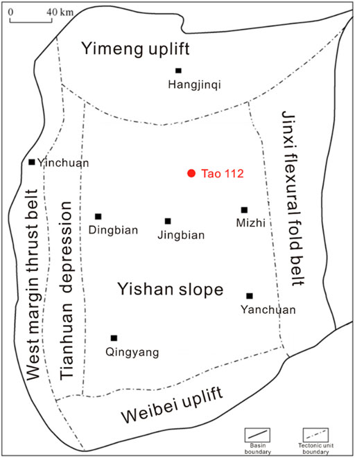
FIGURE 1. Basin structure map and case well located in the study area.

The Majiagou period experienced three major transgression and regression cycles, so the Majiagou Formation can be divided into six lithological sections from bottom to top, of which the Majiagou Member five can be further divided into 10 subsections (Figure 2). The Ma1, Ma3, and Ma5 members are in the regression cycle, which is a limited sea-evaporation shelf environment. Here, dolomites, salt rocks, gypsum rocks, and other evaporites are widely developed. In comparison, the Ma5₆, Ma5₈, and Ma5₁₀ sub-members are in a shorter period of regression. The regressive semi-cycle around the gypsum and salt lagoon is conducive to the formation of high-quality marine source rocks in a highly reducing environment (Wu et al., 2017). The Ma2, Ma4, and Ma6 members are located in the transgressive cycle and are in the epicontinental-marine shelf environment, where micritic limestone and dolomite are widely developed. Due to the late denudation, the Ma6 member is only distributed in the southern part of the basin (Yan et al., 2009).

FIGURE 2

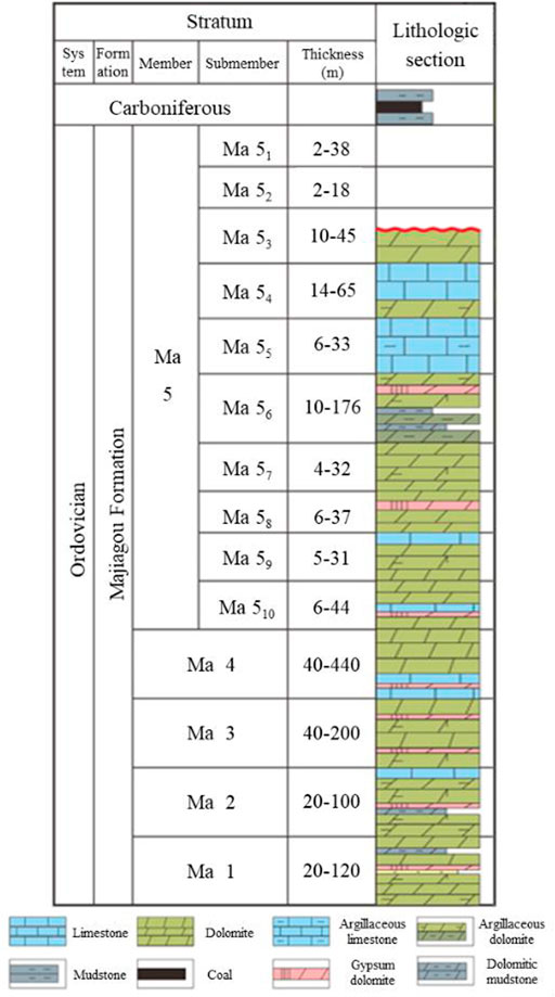
FIGURE 2. Majiagou Formation lithologic histogram.

2.2 Method Principles

2.2.1 Fundamentals of Convolutional Neural Networks

A CNN combines neural networks with deep learning, and neural network models include a convolutional layer. CNNs are composed of numerous neurons. A number of mutually independent neurons form a two-dimensional plane, and a number of two-dimensional planes form a neural-network layer. The multi-layer neural network constitutes the CNN. Compared with BP neural networks, CNNs contain at least one convolutional layer, which is used to extract features. In the convolutional layer, neurons are locally connected and weights are shared, which greatly reduces the computational cost and improves the training efficiency of the neural network. A typical CNN consists of five parts: the input layer, the convolutional layer, the pooling layer, fully connection layer, and the output layer (Figure 3). Among these, the convolutional and pooling layers are unique network structures of CNNs.

1) Convolution layer: This layer removes redundant information through convolutional computation and extracts input data features. The convolutional layer is composed of multiple two-dimensional feature planes, which are connected through the convolutional kernels (Figure 4). The convolution kernel slides from left to right and from top to bottom to carry out the convolution operation step by step; the result is mapped to the convolution layer. The convolution operation can be expressed as

$z_{ij}={\displaystyle \sum _{i=1}^w{\displaystyle \sum _{j=1}^h{A}_{ij}\times B_{ij}}}(1)$

where A_ij denotes the value at the position of row i and column j of the receptive field, B_ij denotes the value at the position of row i and column j of the convolution kernel, and z_ij denotes the output of the convolution kernel at the position of row i and column j. To solve non-linear problems, activation functions, such as the rectified linear activation function $f\left(x\right)=\max \left(0,x\right)$, are usually introduced after the convolution operation to correct the linear unit and improve the generalization ability of the neural network.

FIGURE 3

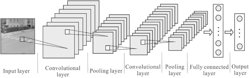
FIGURE 3. Schematic of CNN structure.

FIGURE 4

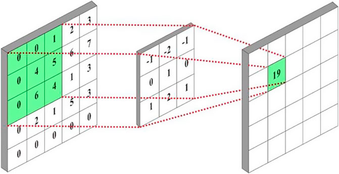
FIGURE 4. Schematic diagram of the convolutional neural network framework.

Figure 4 shows the principle of convolutional operation, where the shaded area in the left-most image is the receptive field, and the shaded area in the right-most image is the result of the convolution calculation.

2) Pooling layer: This layer is usually located after the convolution layer; it is used to reduce the model size and improve the calculation speed. Compared with the original feature map, the pooled feature map has a lower dimension and resolution, by which we can avoid the phenomenon of overfitting. There are two common pooling methods: average pooling and maximum pooling (Figure 5). Average pooling takes the average value of the original image region as the pooled value of the region, whereas maximum pooling takes the maximum value of the original image region as the pooled value of the region. Maximum pooling is usually used in CNNs. Average and maximum pooling can be, respectively, expressed as

$s_{ij}=\frac{1}{c^2} \left({\displaystyle \sum _{i=1}^c{\displaystyle \sum _{j=1}^c{z}_{ij}}}\right)(2)$

$s_{ij}={\mathit{max}}_{ i=1,j=1}^{ c} \left(z_{ij}\right)(3)$

where s_ij denotes the value at the position of row i and column j of the feature image after pooling, c denotes the moving step size of pooling, and z_ij denotes the value at the position of row i and column j of the original feature image.

FIGURE 5

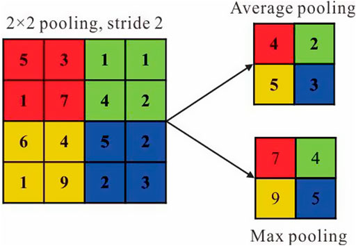
FIGURE 5. Two pooling methods in Convolutional neural network.

The purpose of convolution and pooling in CNNs is to compress and purify the original information, remove redundant information, and improve the generalization ability of the model while improving the training speed.

2.2.2 Convolutional Neural Network Model and Parameter Selection

Logging data are affected by many factors, such as formation lithology, borehole environment, and operation mode, and contain both TOC- related and unrelated information. CNN convolution and pooling operation can purify TOC-related information in logging data while improving the accuracy of TOC calculations.

Logging and TOC data are one-dimensional, so a one-dimensional convolution kernel is used instead of a two-dimensional one. This means that the number of available input parameters of the neural network is reduced, and the pooling layer has little effect on reducing the feature resolution. The designed CNN has five layers (Figure 6). The first layer is the input layer, the second and third layers are the convolutional layers, the fourth layer is the fully connected layer, and the fifth layer is the output layer. According to the correlation analysis, the input layer selects the TOC correlation logging as the input data. In the first layer of convolution, three 2 × 1 convolution kernels (the shadow in Figure 6) are set, and three 2 × 1 feature images can be obtained after convolution. The second level of convolution sets six 3 × 2 × 1 convolution kernels (shadow in Figure 6) and six 1 × 1 feature images can be obtained after convolution. After passing through the full connection layer, the fitting output is carried out. CNN training is divided into two stages: forward propagation and backward propagation. For forward propagation, input data are propagated from the input layer, through the hidden layers, and finally to the output layer, whereas, for backward propagation, the differences between the output and actual values are calculated and the network structure and parameters are adjusted according to the minimum error method until errors are within an allowable range. The optimal model was determined according to the coefficient of determination (R²) and root mean square error (RMSE) between the output and actual TOC values.

FIGURE 6

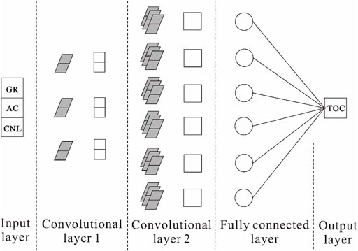
FIGURE 6. Structure diagram of convolutional neural network.

2.2.3 Scheme Design

The Majiagou Formation source rocks in the Ordos Basin are mainly thin dark dolomitic mudstone and argillaceous dolomite, which have strong heterogeneity in the spatial distribution. Well Tao 112 is a whole-section core with abundant logging data, including information related to natural gamma ray, acoustic time difference, neutron porosity, compensated density, and resistivity. Therefore, in this study, core and logging data of Well Tao 112 in the eastern area of the basin were selected as the basic data. After core positioning and logging standardization, 145 groups of TOC measured data and corresponding logging data were obtained.

The original data were standardized and the TOC content and corresponding logging data were selected for correlation analysis. According to the correlation analysis results, TOC-sensitive logging curves were determined as the input parameters of the CNN model. The measured TOC content and the corresponding TOC-sensitive logging curves were used to build a sample database. The constructed samples were inputted into the CNN for training, and CNN parameters were adjusted according to the training effect until the TOC calculation model with the best effect was obtained. Finally, the well logging data were input into the CNN calculation model to obtain the TOC content (Figure 7).

FIGURE 7

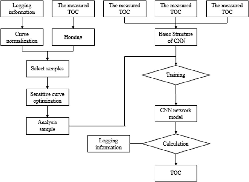
FIGURE 7. CNN-based complex lithology TOC logging calculation process.

The proposed CNN-based TOC logging calculation model takes TOC-sensitive logging curves as input data and outputs TOC content. The sample was randomly divided into two parts, 85% of which were used as training data and 15% as verification data. Overall, 145 datasets were measured for TOC content, 123 of which were used to train the neural network, and the remaining 22 sets were used for verification. To compare the proposed CNN-based TOC logging calculation model with the conventional method, the same data were used to create a control experiment using the multiple regression method.

3 Results and Discussion

3.1 Sensitivity Analysis of Well Logs

The abundance of organic matter in the study area is low, most measured TOC is less than 0.3%, and the response of organic matter is not obvious. The lithology is complex and changeable. Dolomite, limestone, mudstone, salt rock, gypsum rock, and transitional lithology among them are common. The thickness of the lithological layer is thin, and the lithology changes rapidly, thereby making the correlation between logging and TOC content more complex.

Correlation analysis was conducted on the 145 TOC samples and logging data (Figure 8) to determine the logging parameters most sensitive to changes in the TOC content. Natural gamma is closely related to the radioisotope content in the formation, whereas organic matter absorbs uranium (Dong, 2017; Qin et al., 2018), resulting in high-gamma anomalies in the organic-rich formation. Actual data show that TOC content has a positive correlation with natural gamma (Figure 8A), and there is also a certain positive correlation with uranium (Figure 8F).

FIGURE 8

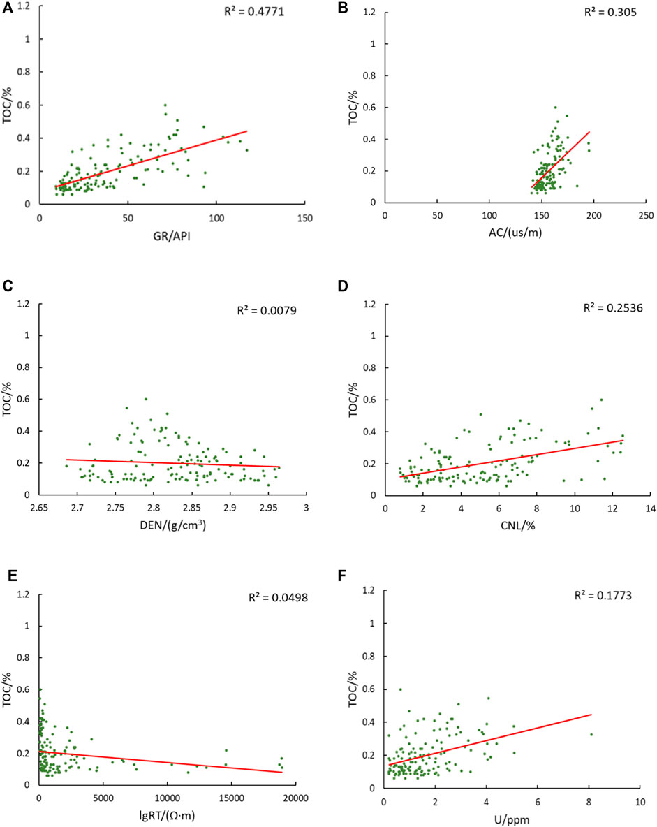
FIGURE 8. Correlation between TOC content and (A) natural gamma ray, (B) acoustic time difference, (C) organic matter density, (D) neutron porosity, (E) formation resistivity, and (F) uranium, 145 samples in each figures.

The kerogen acoustic time difference is greater than the rock-skeleton acoustic time difference, so the formation acoustic time difference increases when the formation is rich in organic matter. Actual data show that the acoustic time difference increases with an increase in TOC content, which suggests a positive correlation between them (Figure 8B).

Generally, the density of organic matter is less than the density of rock skeleton, so the formation density will decrease when organic matter is enriched. The actual data show that the formation density tends to decrease with an increase in TOC content (Figure 8C), but the change is not obvious and may be caused by the low organic matter abundance in the study area.

The neutron porosity is a response to the concentration of hydrogen atoms, and organic matter is rich in hydrogen atoms, so the neutron porosity increases with an increase in TOC content, which suggests a positive correlation between them (Figure 8D).

Generally, the conductivity of kerogen and oil and gas is poor, so formation resistivity increases when organic matter is enriched. Due to the low TOC content of source rocks in the study area, the resistivity is minimally affected by TOC content, and the correlation between them is not obvious (Figure 8E).

According to the above analysis results, TOC content has a strong correlation with natural gamma ray, acoustic time difference, and neutron porosity, but little correlation with density, resistivity, and uranium. Therefore, an accurate prediction model can be established using multiple linear regression. In this experiment, three logging parameters, i.e., natural gamma ray, acoustic time difference, and neutron porosity, were the input parameters of the model. If the linear relationship in this region is not ideal, and because the carbonate source rock itself is very low in organic carbon, machine learning can be used to generate predictions.

3.2 Calculation Results and Comparison

As previously mentioned, 145 samples were obtained with measured TOC calculation model and the remaining 22 values. Of these, 123 samples were used to establish were used to verify the calculation effect of the model. R² and RMSE were used to evaluate the calculation effect. The closer R² is to 1 and RMSE is to 0, the better the calculation effect. According to the measured TOC data and the standardized data of natural gamma-ray, acoustic time difference, and neutron porosity, the multiple regression equation of TOC calculations in this region was obtained using SPSS software. The formula obtained by fitting can be expressed as

$w\left(TOC\right)=0.335\times \mathrm{\Delta }{q}_{API}-0.061\times \mathrm{\Delta }t+0.094\times {\phi }_n+0.098$

where $\Delta q_{API}$ denotes the natural gamma value, ∆t denotes the acoustic time difference, and ${\phi }_n$ denotes the neutron porosity.

On the one hand, concerning the multiple regression method, the R² between the measured and predicted TOC values for the training samples is 0.55, and the RMSE is 7.83% (Figure 9A); for the verification samples, the R² and RSME are 0.23% and 9.18%, respectively (Figure 9B). The interpretation accuracy was 80.583%. It can be seen that the TOC calculation effect of the multiple regression model under the complex lithologic environment is average, and its generalizability is poor. On the other hand, concerning the CNN-based model, the R² between the measured and predicted TOC values of the training samples is 0.83, and the RMSE is 4.80% (Figure 9C); for verification samples, the R² and RSME are 0.86% and 3.60%, respectively (Figure 9D). The interpretation accuracy was 91.589%. Indeed, the CNN-based model is not only highly accurate but also has good generalizability.

FIGURE 9

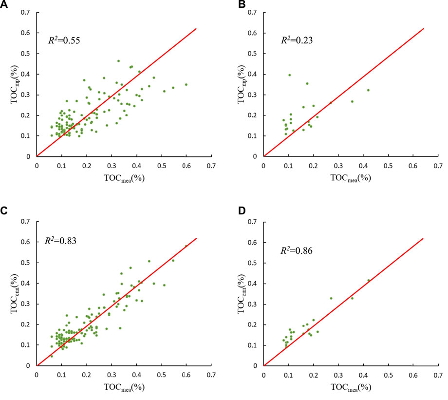
FIGURE 9. The relationship between measured and calculated TOC content. (A) measured- predicted TOC of training samples with multiple linear regression methods (B) measured- predicted TOC of verification samples with multiple linear regression methods (C) measured- predicted TOC of training samples with CNN (D) measured- predicted TOC of verification samples with CNN. TOC_mea denotes the measured TOC content, and TOC_mp and TOC_CNN denote the calculated TOC content using the multiple regression model and the CNN-based model, respectively.

By comparing the calculation results of the multiple regression model and the CNN model (Table 1), from which it is evident that the R² and RMSE of the CNN model are closer to 1 and 0, respectively, indicating that the model is more accurate than the multiple regression model. Moreover, at the level of mathematical indicators, the TOC calculation effect of the CNN model is better than the multiple regression model. By observing the actual TOC calculation effect (Figure 10), the CNN model is more accurate in the context of rapid lithology changes as the multiple regression model can only reflect the overall trend of TOC changes and cannot describe detailed changes. Indeed, when TOC logging calculation is carried out in areas with complex and variable lithology, the TOC calculation effect using CNN will be much better than the traditional multiple regression method, and the predicted TOC distribution will be closer to the actual geological conditions, which is of great significance for future exploration and development.

TABLE 1

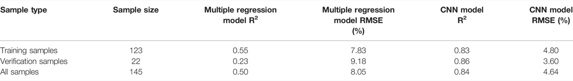
TABLE 1. TOC interpretation results.

FIGURE 10

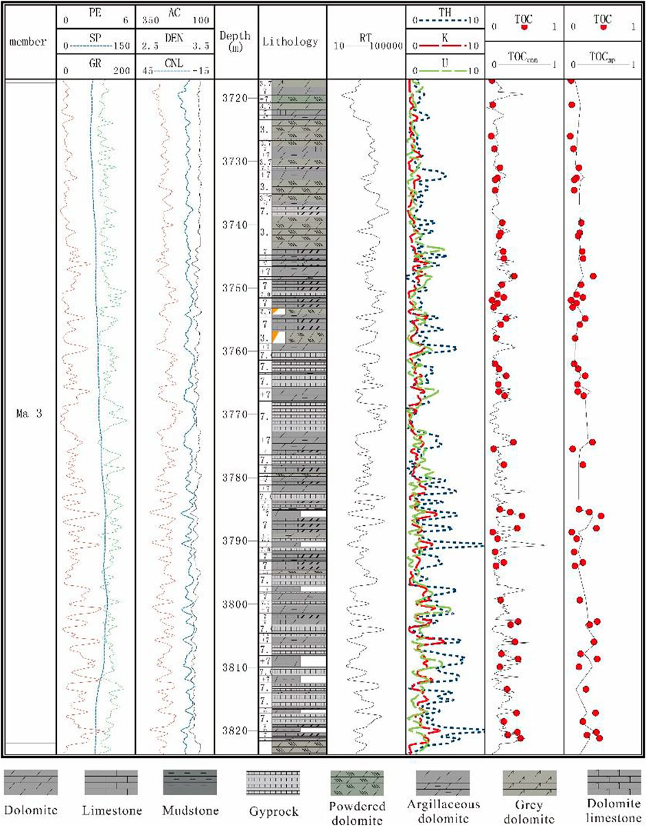
FIGURE 10. TOC results of different models for well Tao 112.

4 Conclusion

A CNN was introduced to TOC logging calculations. The TOC content of Majiagou Formation low-abundance carbonate source rocks in the Tao 112 well area of the eastern Ordos Basin was calculated by multiple regression and CNNs. The research results and related conclusions are outlined below.

(1) In the area with low source rock abundance, the logging response to TOC content was not obvious due to the low TOC content itself. The complexity and variability of lithology further weakened the influence of TOC changes on logging, leading to a generally low correlation between logging and measured TOC content. Therefore, it was difficult to obtain ideal results using multiple regression to calculate TOC content with a linear relationship. The calculation results only reflected the general trend of TOC changes in the vertical direction. In other words, they could not explain detailed TOC changes.

(2) The CNN model can retain the details of TOC changes when calculating TOC in areas with frequent lithologic alternations, and can reflect the changes of TOC more realistically. And its unique weight sharing, local perception and other characteristics make its prediction accuracy higher and adaptability stronger, which can provide a more realistic basis for future exploration and development.

Data Availability Statement

The raw data supporting the conclusions of this article will be made available by the authors, without undue reservation.

Author Contributions

YH: Designed research. ZZ (2nd author): Performed research. XW: analyzed data. ZZ (4th author): analyzed data. WQ: Performed research and wrote the paper.

Funding

This work was financially supported by Science Foundation of China University of Petroleum, Beijing (Grant No. 2462020YXZZ022) and CNPC Innovation Found (No. 2021DQ02-0106).

Conflict of Interest

Author YH was employed by North China oil and gas branch, SINOPEC.

The remaining authors declare that the research was conducted in the absence of any commercial or financial relationships that could be construed as a potential conflict of interest.

Publisher’s Note

All claims expressed in this article are solely those of the authors and do not necessarily represent those of their affiliated organizations, or those of the publisher, the editors and the reviewers. Any product that may be evaluated in this article, or claim that may be made by its manufacturer, is not guaranteed or endorsed by the publisher.

References

Abdel-Hamid, O., Mohamed, A.-r., Jiang, H., Deng, L., Penn, G., and Yu, D. (2014). Convolutional Neural Networks for Speech Recognition. Ieee/acm Trans. Audio Speech Lang. Process. 22, 1533–1545. doi:10.1109/taslp.2014.2339736

CrossRef Full Text | Google Scholar

Chen, A. (2010). Basin Evolution and Sediments Accumulation during Eopaleozoic in Ordos Continental Block. Chengdu, China: Chengdu University of Technology, 147.

Google Scholar

Curiale, J. A. (2017). “Total Organic Carbon (TOC),” in Encyclopedia of Petroleum Geoscience: Cham. Editor R. Sorkhabi (Berlin/Heidelberg, Germany: Springer International Publishing), 1–5. doi:10.1007/978-3-319-02330-4_3-1

CrossRef Full Text | Google Scholar

Dong, H. (2017). Application of Natural Gamma ray Spectrometry Logging. Petrochemical Industry Technol. 24, 260.

Google Scholar

Elkatatny, S. (2019). A Self-Adaptive Artificial Neural Network Technique to Predict Total Organic Carbon (TOC) Based on Well Logs. Arab J. Sci. Eng. 44, 6127–6137. doi:10.1007/s13369-018-3672-6

CrossRef Full Text | Google Scholar

Emelyanova, I., Pervukhina, M., Clennell, M. B., and Dewhurst, D. N. (2016). Applications of Standard and Advanced Statistical Methods to TOC Estimation in the McArthur and Georgina Basins, Australia. The Leading Edge 35, 51–57. doi:10.1190/tle35010051.1

CrossRef Full Text | Google Scholar

Fertl, W. H., and Chilingar, G. V. (1988). Total Organic Carbon Content Determined from Well Logs. SPE Formation Eval. 3, 407–419. doi:10.2118/15612-pa

CrossRef Full Text | Google Scholar

He, K., Zhang, X., and Ren, S. (2016). “Deep Residual Learning for Image Recognition,” in The IEEE conference on computer vision and pattern recognition (CVPR), Las Vegas, NV, USA, 27-30 June 2016, 770–778. doi:10.1109/cvpr.2016.90

CrossRef Full Text | Google Scholar

Huang, Z., and Williamson, M. A. (1996). Artificial Neural Network Modelling as an Aid to Source Rock Characterization. Mar. Pet. Geology. 13, 277–290. doi:10.1016/0264-8172(95)00062-3

CrossRef Full Text | Google Scholar

Karpathy, A., Toderici, G., Shetty, S., and Leung, T. (2014). “Large-scale Video Classification with Convolutional Neural Networks: CVPR '14,” in Proceedings of the 2014 IEEE Conference on Computer Vision and Pattern Recognition, Columbus, OH, USA, June 2014 (Washington, DC: IEEE Computer Society), 1725–1732.

Google Scholar

Khoshnoodkia, M., Mohseni, H., Rahmani, O., and Mohammadi, A. (2011). TOC Determination of Gadvan Formation in South Pars Gas Field, Using Artificial Intelligent Systems and Geochemical Data. J. Pet. Sci. Eng. 78, 119–130. doi:10.1016/j.petrol.2011.05.010

CrossRef Full Text | Google Scholar

Kim, T.-W., and Valdés, J. B. (2003). Nonlinear Model for Drought Forecasting Based on a Conjunction of Wavelet Transforms and Neural Networks. J. Hydrol. Eng. 8, 319–328. doi:10.1061/(asce)1084-0699(2003)8:6(319)

CrossRef Full Text | Google Scholar

Li, L., Wang, L. G., Acero, D. O., and Teixeira, F. L. (2019). “Deep Convolutional Neural Network Approach for Solving Nonlinear Inverse Scattering Problems,” in Proceedings of the IEEE International Symposium on Antennas and Propagation and USNC-URSI Radio Science Meeting, Atlanta, GA, USA, July 2019, 219–220. doi:10.1109/apusncursinrsm.2019.8888813

CrossRef Full Text | Google Scholar

Mahmoud, A. A. A., Elkatatny, S., Mahmoud, M., Abouelresh, M., Abdulraheem, A., and Ali, A. (2017). Determination of the Total Organic Carbon (TOC) Based on Conventional Well Logs Using Artificial Neural Network. Int. J. Coal Geology. 179, 72–80. doi:10.1016/j.coal.2017.05.012

CrossRef Full Text | Google Scholar

Mendelzon, J. D., and Toksoz, M. N. (1985). Source Rock Characterization Using Multivariate Analysis of Log Data, SPWLA 26th Annual Logging Symposium. Dallas, Texas: Society of Petrophysicists and Well-Log Analysts, 21.

Google Scholar

Meng, Z., Guo, Y., and Liu, W. (2015). Relationship between Organic Carbon Content of Shale Gas Reservoir and Logging Parameters and its Prediction Model. J. China Coal Soc. 40, 247–253.

Google Scholar

Meyer, B. L., and Nederlof, M. H. (1984). Identification of Source Rocks on Wireline Logs by Density/resistivity and Sonic Transit Time/resistivity Crossplots1. AAPG Bull. 68, 121–129. doi:10.1306/ad4609e0-16f7-11d7-8645000102c1865d

CrossRef Full Text | Google Scholar

Passey, Q. R., Creaney, S., Kulla, J. B., Moretti, F. J., and Stroud, J. D. (1990). A Practical Model for Organic Richness from Porosity and Resistivity Logs. AAPG Bull. 74, 1777–1794. doi:10.1306/0c9b25c9-1710-11d7-8645000102c1865d

CrossRef Full Text | Google Scholar

Qin, J., Fu, D., Qian, Y., Yang, F., and Tian, T. (2018). Progress of Geophysical Methods for the Evaluation of TOC of Source Rock. Geophys. Prospecting Pet. 57, 803–812.

Google Scholar

Schmoker, J. W. (1979). Determination of Organic Content of Appajacliian Devonian Shales from Formation-Density Logs. AAPG Bull. 63, 1504–1537. doi:10.1306/2f9185d1-16ce-11d7-8645000102c1865d

CrossRef Full Text | Google Scholar

Schmoker, J. W. (1981). Determination of Organic-Matter Content of Appalachian Devonian Shales from Gamma-Ray Logs. AAPG Bull. 65, 1285–1298. doi:10.1306/03b5949a-16d1-11d7-8645000102c1865d

CrossRef Full Text | Google Scholar

Taigman, Y., Yang, M., Ranzato, M. A., and Wolf, L. (2014). “DeepFace: Closing the gap to Human-Level Performance in Face Verification: CVPR '14,” in Proceedings of the 2014 IEEE Conference on Computer Vision and Pattern Recognition, Columbus, OH, USA, June 2014 (Washington, DC: IEEE Computer Society), 1701–1708.

Google Scholar

Wang, J. L., Yang, C. L., and Sun, C. (2009). “A Novel Algorithm for Edge Detection of Remote Sensing Image Based on CNN and PSO,” in Proceedings of the 2009 2nd International Congress on Image and Signal Processing, Tianjin, China, October 2009, 1–5. doi:10.1109/cisp.2009.5304415

CrossRef Full Text | Google Scholar

Wang, X., Yu, S., Li, S., and Zhang, N. (2022). Two Parameter Optimization Methods of Multi-point Geostatistics. J. Pet. Sci. Eng. 208, 109724. doi:10.1016/j.petrol.2021.109724

CrossRef Full Text | Google Scholar

Wu, X., Ding, Z., Yu, Z., Wu, D., and Wang, S. (2017). “Natural Gas Accumulation Conditions and Exploration Potential of the Middle and Lower Assemblages of the Ordovician Majiagou Formation in the Ordos Basin,” in Proceedings of the 2017 National Natural Gas Academic Conference, Hangzhou, Zhejiang, China, May 2017, 15.

Google Scholar

Xie, J., Wu, X., Sun, L., Yu, D., and Wang, S. (2013). Lithofacies Palaeogeography and Potential Zone Prediction of Ordovician Majiagou Member-5 in Ordos Basin. Mar. Origin Pet. Geology. 18, 23–32.

Google Scholar

Xu, G. B., Zhao, G. Y., Yin, L., Yin, Y. X., and Shen, Y. I. (2008). “A CNN-Based Edge Detection Algorithm for Remote Sensing Image,” in Proceedings of the 2008 Chinese Control and Decision Conference, Yantai, China, July 2008, 2558–2561. doi:10.1109/ccdc.2008.4597787

CrossRef Full Text | Google Scholar

Yan, R., Bai, H., Liu, B., and Zhang, S. (2009). Reservoir-forming Conditions of Early Ordovician Majiagou Formation Ma 6 Member, Southern Margin of Ordos Basin. Nat. Gas Geosci. 20, 738–743.

Google Scholar

Yang, H., Griffiths, P. R., and Tate, J. D. (2003). Comparison of Partial Least Squares Regression and Multi-Layer Neural Networks for Quantification of Nonlinear Systems and Application to Gas Phase Fourier Transform Infrared Spectra. Analytica Chim. Acta 489, 125–136. doi:10.1016/s0003-2670(03)00726-8

CrossRef Full Text | Google Scholar

Yu, H., Rezaee, R., Wang, Z., Han, T., Zhang, Y., Arif, M., et al. (2017). A New Method for TOC Estimation in Tight Shale Gas Reservoirs. Int. J. Coal Geology. 179, 269–277. doi:10.1016/j.coal.2017.06.011

CrossRef Full Text | Google Scholar

Zhang, H., Lu, S., Li, W., Tian, W., Hu, Y., He, T., et al. (2017). Application of ΔLogR Technology and BP Neural Network in Organic Evaluation in the Complex Lithology Tight Stratum. Prog. Geophys. 32, 1308–1313.

Google Scholar

Zhao, T., Verma, S., Devegowda, D., and Jayaram, V. (2015). TOC Estimation in the Barnett Shale from Triple Combo Logs Using Support Vector Machine. Tulsa, Oklahoma, United States: Society of Exploration Geophysicists, 791–795. doi:10.1190/segam2015-5922788.1

CrossRef Full Text | Google Scholar

Zheng, M. (2011). Resources and Eco-Environmental protection of Salt Lakes in China. Environ. Earth Sci. 64, 1537–1546. doi:10.1007/s12665-010-0601-8

CrossRef Full Text | Google Scholar

Zhou, J., Xi, S., Deng, H., Yu, Z., Liu, X., Ding, Z., et al. (2020). Tectonic-lithofacies Paleogeographic Characteristics of Cambrian–Ordovician Deep marine Carbonate Rocks in the Ordos Basin. Nat. Gas Industry 40, 41–53.

Google Scholar

Zhu, L., Zhang, C., Zhang, C., Wei, Y., Zhou, X., Cheng, Y., et al. (2019). A Prediction Model for Shale Gas Organic Carbon Content Based on Improved BP Neural Network Using Bayesian Regularization: Geology and Exploration. J. Geophys. Eng. 15 (3), 1050–1061. doi:10.1088/1742-2140/aaa7af

CrossRef Full Text | Google Scholar