A Numerical Experiment of Full Waveform Inversion of Complex Structures Concealed Around a Horizontal Hydraulic Fracturing Well Using Perforation Seismic Data

It is difficult to image the details of complex structures concealed around a horizontal hydraulic fracturing well using seismic data from the ground surface. In this paper, an approach is proposed to solve this problem by non-linear full waveform inversion (FWI) using perforation seismic data. The feasibility of the approach was investigated using numerical modeling based on an experimental model built from the well-known SEG/EAGE overthrust model, which contains complex geological structures with faults. First, seismic modeling was performed to produce experimental synthetic data, including three sets of perforation seismic data recorded by different acquisition systems deployed in observation wells and on the ground surface, and another set of conventional seismic reflection data with both sources and receivers deployed on the ground surface. Then, FWI was performed separately on each data set using an initial velocity model which was heavily smoothed to remove the target structures. The inversion results show that the concealed complex structures around the well were successfully recovered by FWI using perforation data, while the benchmark image from the FWI using conventional seismic data was poor. Particularly, the experiments also demonstrated that FWI using perforation seismic data can image the faults around a horizontal hydraulic fracturing well, while this is unable to achieve using conventional ground surface seismic data. This conclusion was also proved to be valid for noisy data deteriorated either by synthetic Gaussian or field noises. Further experiments demonstrated that FWI using perforation data recorded from wells outperformed that of surface data in terms of structure imaging accuracy characterized by quantitative errors.

Introduction

Concealed complex structures, such as natural faults and fractures, usually exist near injection wells for hydraulic fracturing in shale gas exploitation (Maxwell et al., 2009; Vidic et al., 2013; Clarke et al., 2014; Rutqvist et al., 2017; Ladevèze et al., 2019; Li et al., 2020; Zheng et al., 2020). If these concealed structures are not properly detected before the injection operation, it may lead to serious consequences. For example, leakage of injection fluid can occur and contaminate groundwater during the injecting process (Mair et al., 2012; Flewelling and Sharma, 2014; Edwards et al., 2017; Edwards and Celia, 2018). It may also cause deformation or breakage of horizontal wells (De Pater and Baisch, 2011; Green et al., 2012), or induce earthquakes in natural faults around the injection area (Atkinson et al., 2016; Bao and Eaton, 2016; Ellsworth, 2013; Schultz et al., 2015; Schultz et al., 2018). On the contrary, if the detailed structures could be well detected and seismic velocity of the injection area could be obtained before the injecting process, it will provide not only important information for the injection design but also accurate velocity parameters for the location of microseismic activities induced by the hydraulic fracturing operation (Witten and Shragge, 2017).

It is difficult to obtain the detailed underground structures and accurate seismic velocity in the injection area (Li et al., 2019). Conventional surface seismic reflection exploration can image stratified structures in the injection area (Hennings et al., 2012), but it is difficult to provide details of the concealed complex structures around horizontal wells. Seismic tomography inversion using first arrival time generated by perforation shots or microseismic events can image the macrostructure in the area around horizontal wells (Warpinski et al., 2005; Pei et al., 2008; Pei et al., 2009; Zhang et al., 2009; Bardainne and Gaucher, 2010; Li et al., 2013). However, the details of the structure are difficult to characterize because the seismic phases behind the first break are neglected. These phases carry much information about the detailed features of the complex structures. Comparatively, full waveform inversion (FWI) makes full use of waveform, which contains not only the information of arrival time but also the dynamic effects of the media applied on the waves. This information of the seismic data is of great help for the recovery of the complex structures with high accuracy (Virieux and Operto, 2009; Sirgue et al., 2010; Operto et al., 2015; Virieux et al., 2017).

FWI is a non-linear inversion method. It normally requires high-quality data with a high signal-to-noise ratio (S/N) and an initial velocity model with good approximation to the actual velocity structure. In this regard, offshore seismic exploration has the advantage, and most applications of FWI are implemented to offshore seismic data (Operto et al., 2015; Sirgue et al., 2010; Virieux et al., 2017). In contrast, the shallow surface conditions of onshore seismic exploration are much more complex and would result in lower S/N ratio data. It is difficult for FWI to recover the detailed geological structures with noisy data (Zhang et al., 2016). In addition, if the hydraulic injection site is in a densely populated or rugged mountain area, it is difficult to use an ideal acquisition system for surface seismic reflection exploration. This will result in the hidden complex structures near horizontal wells being inadequately illuminated. However, if seismic sources can be placed below these hidden complex structures, the energy of the source can directly pass through these structures and be recorded by geophones on the ground surface or in observation wells. This will greatly improve the illumination of the hidden complex structures. For this reason, we propose to use an FWI scheme to invert the detailed structures around the horizontal well using perforation data as its sources are located along the horizontal well. Receiving geophones can be deployed on the ground surface, if conditions are permitted or deployed in observation wells to record seismic data. When the location and onset time of the perforation shots are generally known (Pei et al., 2009; Tan et al., 2014), this excitation and acquisition configuration is promising for FWI to invert the complex structures around the horizontal well.

Experiments

Theory

The goal of FWI is to approach the target model by iteratively updating the initial model. In the iterative process, the difference between the synthetic and observed data is gradually reduced to an acceptable level. A classic misfit function of FWI can be defined as an L₂ norm:

$E=\frac{1}{2}{\displaystyle \sum _{Ns}{\displaystyle \sum _{Nr}{\Vert \mathbf{d}-\mathbf{u}\Vert }^2}},(1)$

where Ns and Nr are the number of sources and receivers, respectively, d represents the observed data, and u represents the synthetic data, which is a function of the medium parameter $m\left(\mathbf{r}\right)$ at the current iterative FWI updating stage and can be synthesized by wave equation modeling.

The minimization problem of Eq. 1 requires calculating the gradient direction of E with respect to the model parameter $m$ as a variable during the iterative process of FWI, i.e., $\partial E/\partial m$. A quick and effective way to compute the gradient is using the adjoint-state method (Plessix, 2006):

$\frac{\partial E}{\partial m}=-{\displaystyle \sum _{Ns}{\displaystyle \underset{0}{\overset{T}{\int }}{\lambda }_s\frac{{\partial }^{2}u}{\partial t^2}dt}},(2)$

where ${\lambda }_s$ is the back-propagating residual wavefield, i.e., d-u. Thus, the conjugate gradient method (Hestenes and Stiefel, 1952) is used to update the model iteratively:

${\mathbf{m}}_{k+1}={\mathbf{m}}_k+{\alpha }_k{\mathbf{p}}_k,(3)$

here the vector ${\mathrm{m}}_k$ denotes the parameter model at the $k^{th}$ step during the FWI iterative process, and α and p are the step length and the search direction, respectively, for the updating change of the model. We can use the inexact linear search method (Nocedal and Wright, 2006) to obtain α. For p, we can use the method of Dai and Yuan (1999):

${\mathbf{p}}_{\mathit{k}\mathrm{+1}}=-q_{k+1}^{{\rm T}}{\left(\frac{\partial E}{\partial \mathbf{m}}\right)}_{k+1}+{\beta }_{k+1}{\mathbf{p}}_k,(4)$

where $\frac{\partial •}{\partial \mathrm{m}}\triangleq {\left(\frac{\partial •}{\partial m\left({\mathrm{r}}_1\right)},\frac{\partial •}{\partial m\left({\mathrm{r}}_2\right)},\cdots ,\frac{\partial •}{\partial m\left({\mathrm{r}}_n\right)}\right)}^T$ with ${\mathrm{r}}_i,i=\mathrm{1,2},\cdots ,n$ being the spatial position vector, T is the matrix transpose, and q is a preconditioning operator (Plessix and Mulder, 2004; Shin et al., 2001):

$q_k={\left\{{\displaystyle \underset{0}{\overset{T}{\int }}{\left|\mathbf{u}\left(\mathbf{m},t\right)\right|}^{2}dt}\right\}}^{-1}.(5)$

β in Eq. 4 is a scalar, which can be obtained by the method of Dai and Yuan (1999):

${\beta }_k=\frac{{\left(\frac{\partial E}{\partial \mathbf{m}}\right)}_{k+1}^{{\rm T}}{\left(\frac{\partial E}{\partial \mathbf{m}}\right)}_{k+1}}{{\mathbf{p}}_k^{{\rm T}}\left\{{\left(\frac{\partial E}{\partial \mathbf{m}}\right)}_{k+1}-{\left(\frac{\partial E}{\partial \mathbf{m}}\right)}_k\right\}},(6)$

Modeling

Geological Model

A two-dimensional velocity model (Figure 1) was extracted from the well-known SEG/EAGE overthrust model (Aminzadeh et al., 1994) for our experiments. The horizontal dimension of the model is 4 km, the depth dimension is 2 km, and the P-wave velocity ranges from 2.0 to 6.5 km/s. There exist complex fold structures with faults in the model. There are three wells within the model area (Figure 1), including a horizontal well laying at the depth of 1.5 km, and two vertical observation wells on the horizontal coordinates of 0.5 km, on the left side, and 3.5 km, on the right side, separately. The design of the horizontal well is referred to the statistics of Edwards and Celia (2018), the depths of horizontal wells are normally between 1.5 and 3.0 km, the length is 1.0–3.0 km, and the spacing of perforation shots is 20–40 m.

FIGURE 1

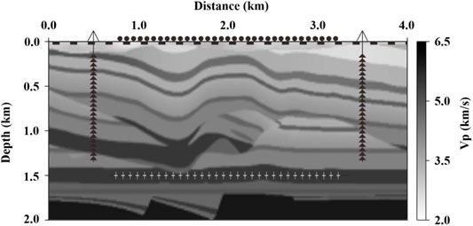
FIGURE 1. Overthrust model with concealed structures. The black solid lines are the trajectories of the vertical observation wells and horizontal wells. The solid black circles at the top of the model represent the surface seismic sources. The black dashed line represents the receivers. The black triangles represent the receivers in the two wells located at x = 0.5 and 3.5 km, respectively. The white cross symbols represent the perforations in the horizontal well which is located at the depth of z = 1.5 km. These form an acquisition system covering the complex fold structures with faults in the model.

Acquisition Systems

To compare the inversion results of perforation and surface seismic reflection data, four acquisition systems were designed:

1) surface excitation and surface recording (SS);

2) perforation excitation and surface recording (PS);

3) perforation excitation and one well recording (PO);

4) perforation excitation and two well recording (PT).

There are 125 conventional seismic sources on the ground surface (the solid black circles at the top of the model in Figure 1) for the SS acquisition system, and the same number of perforation sources in the horizontal well (the white crosses in the horizontal well at the depth of 1.5 km) were used for the acquisition systems of PS, PO, and PT. All sources are distributed horizontally in the range of 0.75–3.25 km with a space interval of 20 m.

To record two-component velocity data (Vx and Vz represent the horizontal and vertical velocity components, respectively), 65 two-component receivers are deployed on the ground surface spanning 0.06–3.9 km (the black dashed line in Figure 1), with a spatial interval of 60 m. Similarly, 25 receivers are deployed in each observation well in the depth ranging between 0.1 and 1.3 km (the black triangles in Figure 1), with a spacing interval of 50 m.

Synthetic Data

The velocity model in Figure 1 is discretized using a spacing interval of 20 m in both horizontal and vertical directions. The total number of grid points is 200*100 = 20000. For forward modeling, a free surface boundary condition is used at the top of the model. The perfectly matched boundary condition (PML) with a thickness of 10 grid points is adopted on the other three sides. A pulse function with a frequency band of 0–20 Hz is used as the source signal. The time sampling interval for forward modeling is 0.5 ms. The total time history of the modeling is 2.5 s. The wavefields are solved using the method of Köhn (2011). The synthetic seismograms of the velocity components (i.e., Vx and Vz) are recorded by the observation system of SS, PS, PO, and PT, which will be used as the names of the data sets in the following context. The wavefields recorded are shown in Figure 2.

FIGURE 2

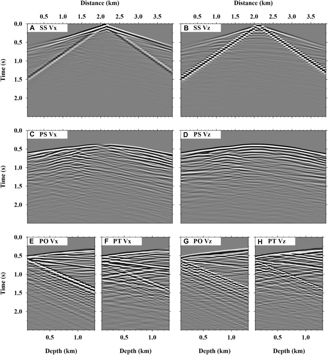
FIGURE 2. Synthetic seismograms. (A,B) are the Vx and Vz components, respectively, of SS. Similarly, (C,D) are of PS, (E,G) are of PO, and (F,H) are of PT. The data of PT were recorded using the array on the vertical well on the right-hand side of the model.

Results

FWI software used in this study was developed based on the open codes published by Köhn et al. (2012). The initial velocity model (Figure 3) used for the modeling was obtained by applying Gaussian smoothing (σ = 20, radius = 50) to the exact velocity model, as shown in Figure 1. After smoothing, the complex structures in Figure 1 completely disappeared.

FIGURE 3

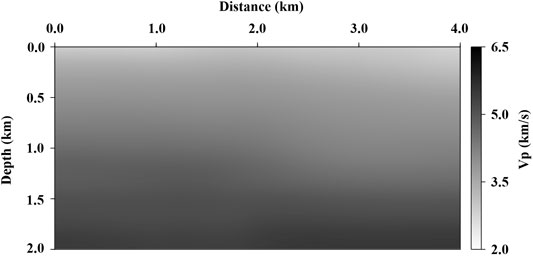
FIGURE 3. Initial velocity model obtained by applying Gaussian smoothing to the exact model shown in Figure 1.

An inversion frequency range of 0–20 Hz is used to cover the effective frequency band of the synthetic data. It is organized into 10 groups, namely, 0–2 Hz, 0–4 Hz, and so on up to 0–20 Hz. FWI is first performed on the frequency ground of 0–2 Hz with the initial model shown in Figure 3. The final inversion model of 0–2 Hz was used as the initial model for the next inversion performed on 0–4 Hz. The inversion is progressively performed in such a manner from low to high frequencies until the inversion of the last frequency group (0–20 Hz) is completed. This inversion strategy was adopted from Virieux and Operto (2009) to reduce the instability of the non-linear inversion accordingly.

Using the data sets of SS, PS, PO, and PT (Figure 2) separately, the inversion results in four corresponding images of the hidden complex structures near the horizontal well are shown in Figures 4–7. Each image shows the progressive results of 0–2, 0–8, 0–14, and 0–20 Hz. It can be seen that the inversion result of the first frequency group (0–2 Hz) of SS (Figure 4A) is the same as the initial model, without showing the definite structure (Figure 4A). When the frequency reaches up to 8 Hz, the stratum where the horizontal well is located and the buried fault above the horizontal well begin to appear (arrows in Figure 4B). With the frequency inversion continuing up to 14 Hz, the folds and faults are well recovered (Figure 4C). When the frequency reaches 20 Hz, the inversion results have reached a steady state. The shape of the overburden stratum structure of the horizontal well is removed, but the spatial resolution of the overthrust fault near the horizontal wells is very low (arrows in Figure 4D).

FIGURE 4

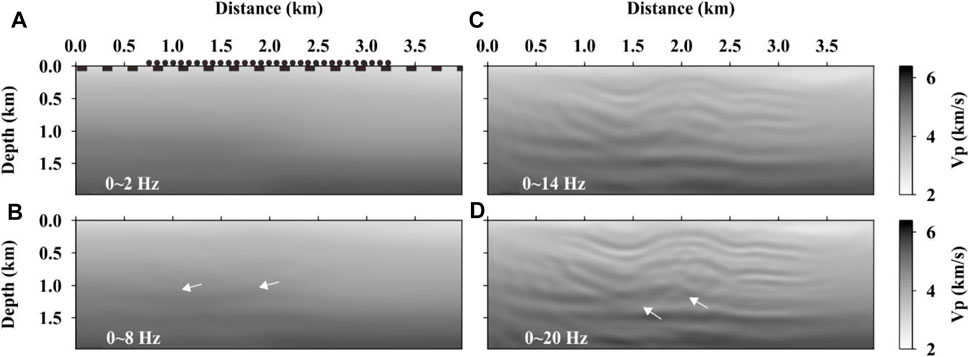
FIGURE 4. Inversion results of SS data. The acquisition system is represented by the solid black circles (sources) and dashed line of blocks (receiver array) at the top of (A). (A–D) Iterative inversion results as gray images of the frequency groups of 0–2, 0–8, 0–14, and 0–20 Hz, respectively.

Figure 5 shows the inversion results of the PS data. From the inversion results of the 0–2 Hz data (Figure 5A), the low-frequency components mainly recover the large-scale structures between the receiver array (black dashed line) and the perforations (black plus symbols). With the 8 Hz data, not only the folded strata can be imaged but also the deep faults are well recovered (arrows in Figure 5B). When the inversion frequency reaches 14 Hz, the overall structure becomes significantly clearer (Figure 5C). When the inversion reaches the last frequency group of 0–20 Hz (Figure 5D), the results are only slightly improved from that of 14 Hz (arrows in Figure 5D), indicating that the inversion reaches a stable stage in the frequency band above 14 Hz.

FIGURE 5

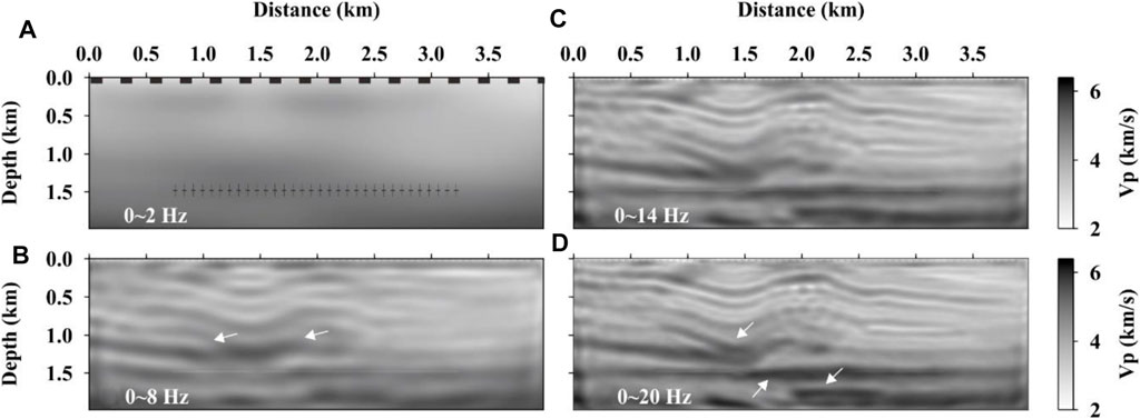
FIGURE 5. Inversion results of the PS data. (A) Dashed line of black blocks at the top represents receivers, and the black cross symbols at the depth level of 1.5 km represent the perforations in the horizontal well. (A–D) Iterative inversion results of the frequency groups of 0–2, 0–8, 0–14, and 0–20 Hz, respectively.

The inversion results of the PO data are shown in Figure 6. The inversion results of 0–2 Hz data (Figure 6A) show velocity updates in the area near the vertical observation well. When the frequency reaches 8 Hz, the shallow folded strata and deep faults have been successfully recovered (Figure 6B). When the inversion frequency reaches 14 Hz, the overall structure of the model on the observation side is clearer than that of 8 Hz. In addition, the velocity accuracy is also further improved (Figure 6C). Similar to that of PS, only a slight improvement is achieved when the inversion reaches the last frequency group of 0–20 Hz (Figure 6D), indicating that the inversion reaches a stable stage in the frequency band above 14 Hz.

FIGURE 6

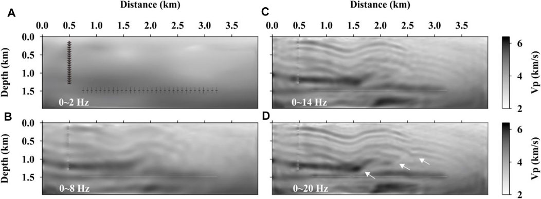
FIGURE 6. Inversion results of the PO data. The black triangles on the left and the black cross symbols at the depth level of 1.5 km shown in (A) represent the receivers in the observation well and the perforations in the horizontal well, respectively. (A–D) Iterative inversion results of the frequency groups of 0–2, 0–8, 0–14, and 0–20 Hz, respectively.

The PT data results (Figure 7) show that the inversion of the 0–2 Hz data is updated over the whole model, as it would be anticipated as the receivers now deployed on both sides compared with the signal side receiving of PO. However, the outline of the structure is yet not evident (Figure 7A). When the inversion frequency reaches 8 Hz, the result clearly shows the shallow folded strata and deeply buried faults (Figure 7B). The imaging quality at this frequency band is better than that of SS (Figure 4B), PS (Figure 5B), and PO (Figure 6B), indicating that the inversion convergence of PT is faster than the others. With the frequency reaching 14 Hz, most of the structures have been recovered (Figure 7C). When the inversion reaches the final frequency group (Figure 7D), the spatial resolution of the whole structure is further improved and the result is very close to the real model (Figure 1).

FIGURE 7

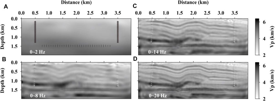
FIGURE 7. Inversion results of the PT data. Black triangles on each side and the black cross symbols at the depth level of 1.5 km in (A) represent the receivers in the vertical observation well and the perforations in the horizontal well, respectively. (A–D) Iterative inversion results of frequency groups of 0–2, 0–8, 0–14, and 0–20 Hz, respectively.

Analysis and Discussions

Error Analysis

To look into the detailed difference between the inversion results of the four data sets, the absolute error between each inverted velocity model (Figures 4–7) and the actual velocity model (Figure 1) was calculated (Figure 8). It shows that SS has a very large error (Figure 8A). The error of PS near the horizontal well is smaller than that of SS (Figure 8B). Although the error of PO is small in the area near the observation well on the left (Figure 8C), the error of PT is the smallest over the whole model compared to other data sets, indicating that PT outperforms PO and PS (Figure 8D).

FIGURE 8

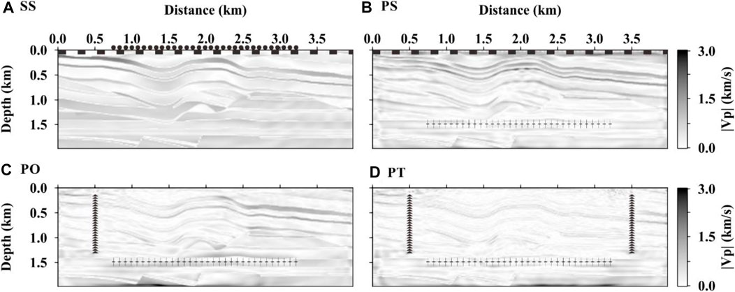
FIGURE 8. Absolute error of the final inverted velocity models relative to the actual velocity model. As marked at the top left corner of each panel, (A–D) Errors of SS, PS, PO, and PT data, respectively.

The velocity profiles versus depth at locations of distances 1.0, 2.0, and 3.0 km are extracted from the inverted models. Along with the initial model, the profiles are shown against the exact model in Figure 9, to demonstrate the difference variation versus depth. It can be seen that the inversion results of the SS data (solid blue line) are largely different from the exact model. Although the inversion from the PS data (solid cyan line) is poor in the shallow region above the depth of 0.5 km, it is in good agreement with the actual velocity structure below 0.5 km. The inversion results of PO (solid green line) in the area near the observation well on the left (Figure 9A) are in good agreement with the exact model, and the results far away from the observation well area are very poor (Figure 9C). All inversion results for PT (solid red line) are close to the exact curves, which mean PT delivers the best inversion.

FIGURE 9

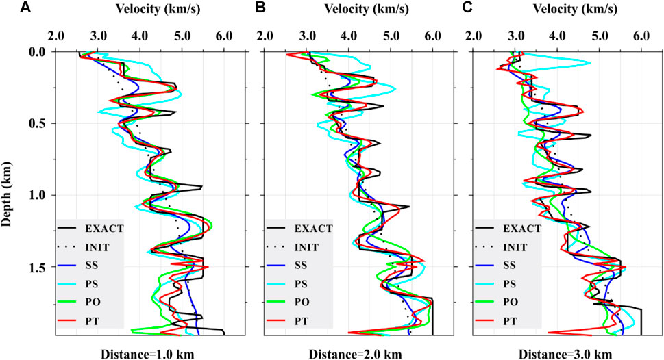
FIGURE 9. Velocity profiles versus depth from the inversion results at distances of 1.0 km (A), 2.0 km (B), and 3.0 km (C). Velocity profiles of the initial model and the actual model are also plotted as references.

Anti-Noise Performance

The conclusions above are based on the experiment using noise-free data. Considering that field seismic data usually contain a certain degree of noise, we use noisy data to test the validity of the conclusions.

The first experiment concerns Gaussian noise, which is generated and added into the seismogram (Figure 2) to synthesis noisy seismic data with S/N = 2.0 (Figure 10). The S/N used is defined as the ratio of the root-mean-square (RMS) amplitude of noise-free data (shown in Figure 2) to random noise for each trace. Comparing Figure 10 with Figure 2, most of the signals of SS (a and b), PS (c and d), PO (e and g), and PT (f and h) are submerged in noise.

FIGURE 10

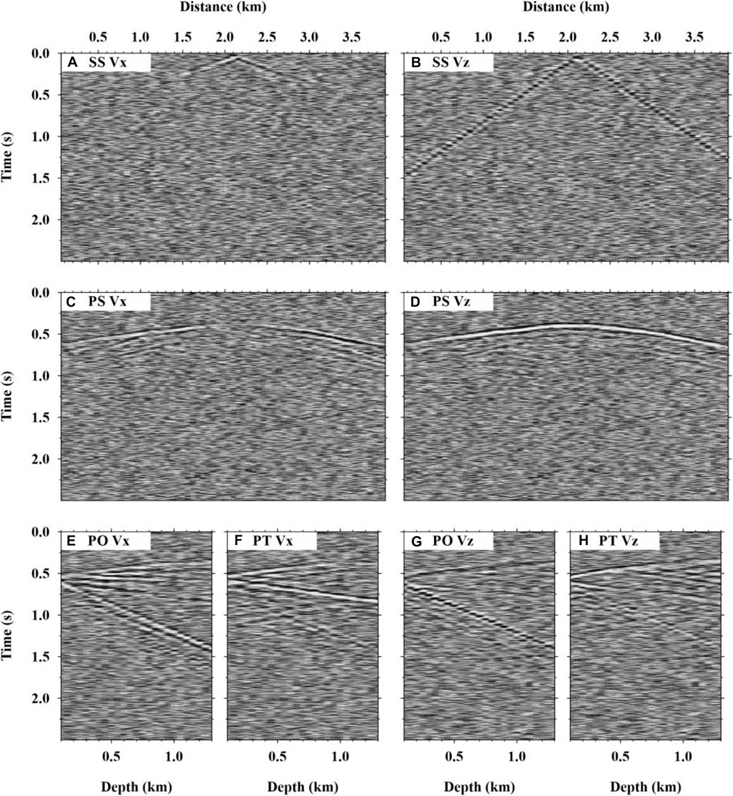
FIGURE 10. Noisy data with S/N = 2.0 synthesized by adding Gaussian to the Vx and Vz seismograms of SS (Plots A and B), PS (Plots C and D), PO (Plots E and G), and PT (Plots F and H), as shown in Figure 2. The seismograms of PT were recorded using the array deployed on the vertical well on the right-hand side of the model.

The noisy data, as shown in Figure 10, were then used for the FWI inversion in the same way as the previous inversion experiment. The results alongside their absolute errors from the actual velocity model are shown in Figure 11. Compared with the noise-free results (Figures 4–7), the structural characterization accuracy of the final inversion results of the noisy data is deteriorated for all data of SS, PS, PO, and PT (Figures 11A,C,E,G). The final inversion results of SS data only show the outline shape of the shallow folded strata (Figure 11A). The complex structures near the horizontal well are obscured. Moreover, the overall velocity error of SS is large (Figure 11B). The inversion results of PS data recover the general shape of the nappe structures near the horizontal well (Figure 11C), but there are very large errors in the shallow part (Figure 11D). By using PO data, the inversion can recover the structure near the observation well (Figure 11E) with small errors (Figure 11F). The reconstructed structures using the PT data (Figure 11G) are in good agreement with the exact model (Figure 1). Compared with SS, PS, and PO, PT has the smallest overall velocity error (Figure 11H). These results confirm that the previous conclusions from the noise-free data are valid for data deteriorated by Gaussian noise.

FIGURE 11

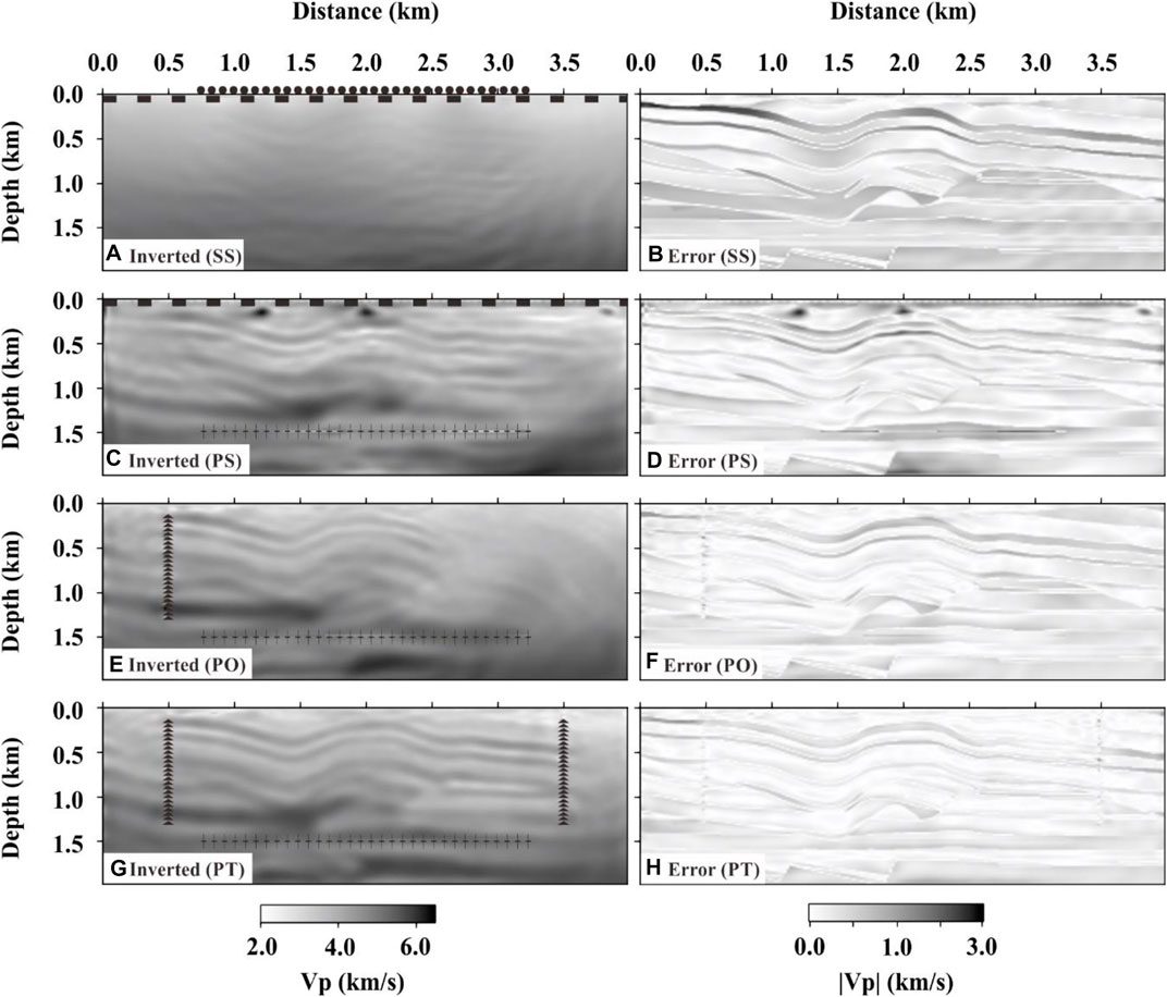
FIGURE 11. Inversion results (Blocks A, C, E and G in the column on the left-hand side) of data contaminated with Gaussian noise (S/N = 2.0) and the absolute velocity error (Blocks B, D, F and H in the column on the right-hand side) relative to the actual velocity model. The results of SS, PS, PO, and PT data are marked in the bottom left corner of each block.

The second experiment concerns field noise. The Gaussian noise was replaced by the field noise recorded from the Upper Yangtze area of China. This field noise includes not only the natural random noise but also human activities and machine operations on site. Before adding the field noise to the synthetic data (Figure 2), a frequency band pass filtering is processed to keep it consistent with the data. The noise is added in such a proportion that the resultant noisy data are of S/N = 2.0. As seen from Figure 12, the noisy seismic records contain large amplitude noise randomly distributed in the profiles.

FIGURE 12

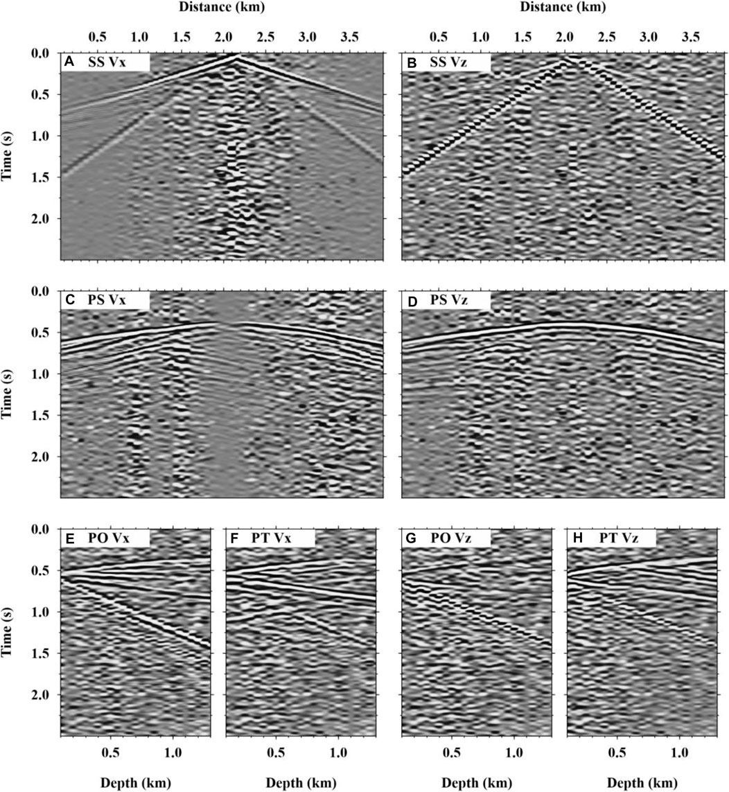
FIGURE 12. Noisy data with S/N = 2.0 synthesized by adding field noise to the Vx and Vz seismograms of SS (Plots A and B), PS (Plots C and D), PO(Plots E and G), and PT (Plots F and H), as shown in Figure 2. The seismograms of PT are recorded using the array on the vertical well on the right-hand side of the model.

Using the same inversion procedures as for the previous experiments concerning Gaussian noise, we obtained the inversion results and their velocity errors against the actual model (Figure 13). From the structures near the horizontal wells, the results of Figure 13 are consistent with that of the Gaussian noise shown in Figure 12. The inversion result of SS (Figure 13A) cannot clearly reflect the complex structure near the horizontal well and the error is the largest (Figure 13B). The results of PO (Figure 13E) recover most of the overthrust structures above the horizontal well. Its velocity error is much smaller than that of SS (Figure 13F). The results of PS (Figures 13C,D) are similar to those of PT (Figures 13G,H), but PT has the best agreement with the exact velocity model. It further confirms that the previous conclusions obtained from the noise-free data hold valid not only for data deteriorated by Gaussian noise but also by random field noise.

FIGURE 13

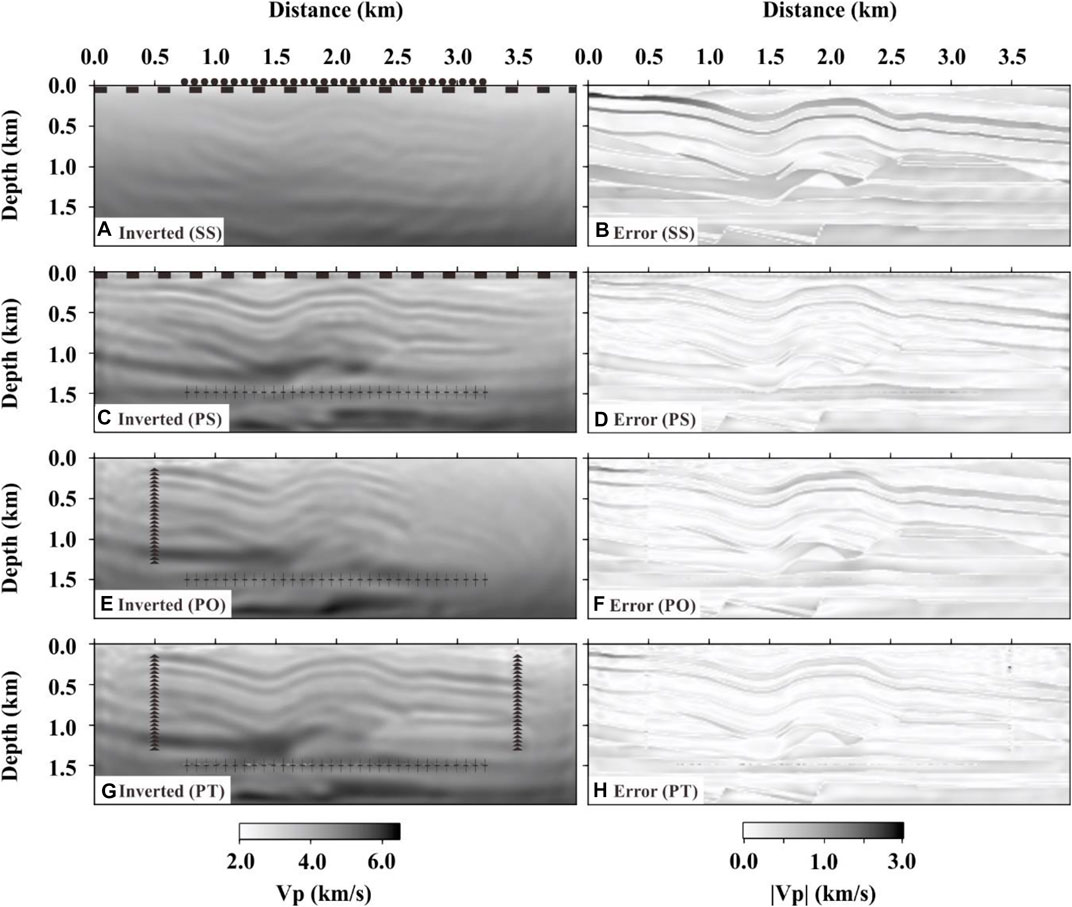
FIGURE 13. Inversion results (left) and absolute velocity error (right) of SS, PS, PO, and PT data with field noise (S/N = 2). (A) Result of SS. (B) Absolute error between the inverted velocity in (A) and the exact velocity (Figure 2). Similarly, (C,D) are from PS, (E,F) from PO, and (G,H) from PT. The results of SS, PS, PO, and PT data are marked in the lower left corner of each block and presented in order from the top to the bottom.

Fault Imaging

To achieve the goals of a hydraulic fracturing operation, it is desirable to image the faults around a horizontal hydraulic fracturing well. In the previous modeling experiments, there are complex fault structures around the horizontal hydraulic fracturing well (arrows in Figure 14A). To demonstrate the ability of FWI to image these faults using perforation seismic data, a comparison of the FWI results of SS, PS, PO, and PT data contaminated by the field noise (S/N = 2.0) is shown in Figure 14. No sign of the faults is seen in the FWI results of SS (Figure 14B). This means the faults cannot be imaged using conventional ground surface seismic data. On the contrary, the faults are successfully recovered in the FWI results of PS, PO, and PT data (See the red arrows in Figures 14C–E, respectively). Among the results of PS, PO, and PT, the ability of using PS data to image faults is limited (black arrows in Figure 14C). In addition, PO produces a sharper image of the fault structures near the receiving array (red arrows in Figure 14D), while the image of the faults far away from the receiving array is poor. In contrast, the PT image showed the most accurate shapes and locations of all the faults (red arrows of Figure 14E).

FIGURE 14

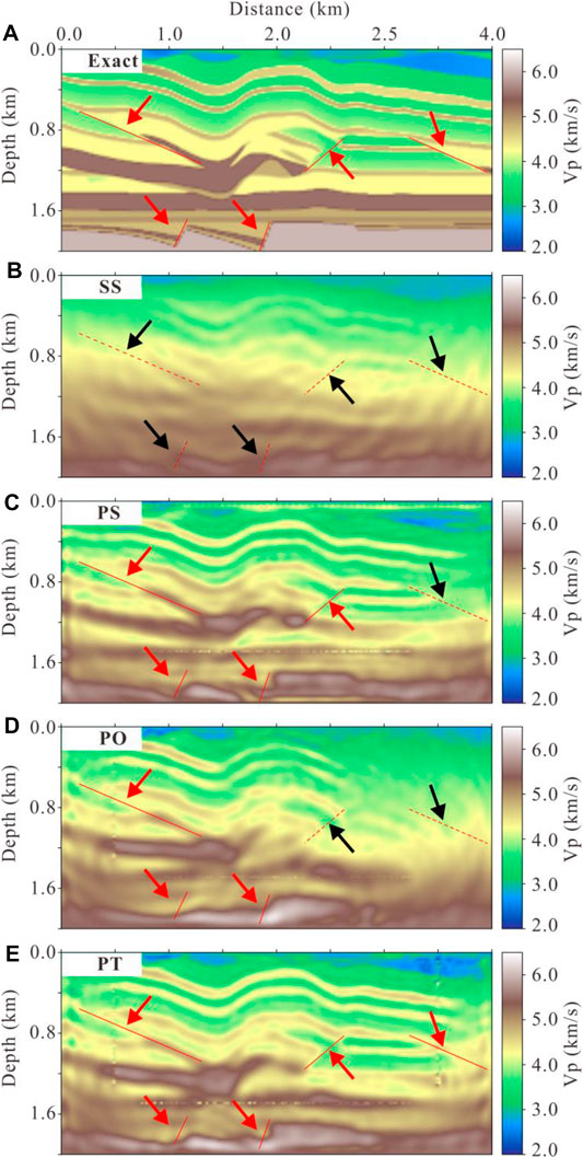
FIGURE 14. Comparison of fault structures from the exact velocity model (A). Inversion results of SS (B), PS (C), PO (D), and PT (E). Red arrows in (A) indicate the location of complex fault structures (solid red lines). (B–E) Red arrows indicate the successfully imaged fault structures (solid red lines), while the black arrows indicate fault structures that failed to recover (dashed red lines).

It is worth to pointing out that the strategy given in this article mainly focuses on the inversion of macroscopic structures. It is theoretically possible to image micro-scale fractures under ideal conditions. However, this would require a very dense array of observation systems capable of receiving very effective frequency data, which would be very challenging technically and unbearable economically.

Conclusions

In this article, we proposed an FWI strategy for the inversion of concealed complex structures around a horizontal well using perforation seismic data. Numerical experiments were used to test the feasibility of the strategy. Perforation seismic data recorded from the ground surface and the observation wells were separately used in the inversion. As a benchmark, inversion is also performed using conventional reflection seismic data from the ground surface. The results show that:

(1) The FWI inversion of using perforation seismic data to image the concealed complex structures around horizontal wells is successful. The inversion images of perforation data showed clear details of the structures that cannot be imaged clearly with conventional reflection seismic data.

(2) The validity of this FWI strategy was further proved by the anti-noise performance experiments using data heavily contaminated with Gaussian or field noise. Inversions using perforation data from observation wells outperformed using data from the ground surface.

(3) The experiments also demonstrated that FWI using perforation seismic data could image the faults around a horizontal hydraulic fracturing well, while this was unable to achieved using conventional ground surface seismic data.

In summary, the modeling experiments demonstrate that the proposed FWI strategy for imaging concealed complex structures around a horizontal well using perforation seismic data is feasible. Compared with using conventional seismic data from the ground surface, this strategy has significant advantages in imaging resolution and anti-noise performance.

Data Availability Statement

The original contributions presented in the study are included in the article/supplementary material, further inquiries can be directed to the corresponding author.

Author Contributions

GQ, JLY and XF are responsible for the experiments, of which the plan was designed together with JSY, and the initial draft of the manuscript, which was later rewritten by JSY with further analysis of experiment results.

Funding

This work was funded by the Open Fund (PLC2020060) of the State Key Laboratory of Oil and Gas Reservoir Geology and Exploitation (Chengdu University of Technology), China and the National Natural Science Foundation of China (Grant Number 41774059).

Conflict of Interest

The authors declare that the research was conducted in the absence of any commercial or financial relationships that could be construed as a potential conflict of interest.

Publisher’s Note

All claims expressed in this article are solely those of the authors and do not necessarily represent those of their affiliated organizations, or those of the publisher, the editors, and the reviewers. Any product that may be evaluated in this article, or claim that may be made by its manufacturer, is not guaranteed or endorsed by the publisher.

References

Aminzadeh, F., Burkhard, N., Nicoletis, L., Rocca, F., and Wyatt, K. (1994). SEG/EAEG 3-D Modeling Project: 2nd Update. The Leading Edge 13 (9), 949–952. doi:10.1190/1.1437054

CrossRef Full Text | Google Scholar

Atkinson, G. M., Eaton, D. W., Ghofrani, H., Walker, D., Cheadle, B., Schultz, R., et al. (2016). Hydraulic Fracturing and Seismicity in the Western Canada Sedimentary Basin. Seismological Res. Lett. 87 (3), 631–647. doi:10.1785/0220150263

CrossRef Full Text | Google Scholar

Bao, X., and Eaton, D. W. (2016). Fault Activation by Hydraulic Fracturing in Western Canada. Science 354 (6318), 1406–1409. doi:10.1126/science.aag2583

PubMed Abstract | CrossRef Full Text | Google Scholar

Bardainne, T., and Gaucher, E. (2010). Constrained Tomography of Realistic Velocity Models in Microseismic Monitoring Using Calibration Shots. Geophys. Prospecting 58 (5), 739–753. doi:10.1111/j.1365-2478.2010.00912.x

CrossRef Full Text | Google Scholar

Clarke, H., Eisner, L., Styles, P., and Turner, P. (2014). Felt Seismicity Associated with Shale Gas Hydraulic Fracturing: The First Documented Example in Europe. Geophys. Res. Lett. 41, 8308–8314. doi:10.1002/2014gl062047

CrossRef Full Text | Google Scholar

Dai, Y. H., and Yuan, Y. (1999). A Nonlinear Conjugate Gradient Method with a strong Global Convergence Property. SIAM J. Optim. 10 (1), 177–182. doi:10.1137/s1052623497318992

CrossRef Full Text | Google Scholar

De Pater, C., and Baisch, S. (2011). Geomechanical Study of Bowland Shale Seismicity. Synth. Rep. 57.

Google Scholar

Edwards, R. W. J., and Celia, M. A. (2018). Shale Gas Well, Hydraulic Fracturing, and Formation Data to Support Modeling of Gas and Water Flow in Shale Formations. Water Resour. Res. 54 (4), 3196–3206. doi:10.1002/2017wr022130

CrossRef Full Text | Google Scholar

Edwards, R. W. J., Doster, F., Celia, M. A., and Bandilla, K. W. (2017). Numerical Modeling of Gas and Water Flow in Shale Gas Formations with a Focus on the Fate of Hydraulic Fracturing Fluid. Environ. Sci. Technol. 51 (23), 13779–13787. doi:10.1021/acs.est.7b03270

PubMed Abstract | CrossRef Full Text | Google Scholar

Ellsworth, W. L. (2013). Injection-induced Earthquakes. Science 341 (6142), 1225942. doi:10.1126/science.1225942

PubMed Abstract | CrossRef Full Text | Google Scholar

Flewelling, S. A., and Sharma, M. (2014). Constraints on Upward Migration of Hydraulic Fracturing Fluid and Brine. Groundwater 52 (1), 9–19. doi:10.1111/gwat.12095

CrossRef Full Text | Google Scholar

Green, K. W., Zelbst, P. J., Meacham, J., and Bhadauria, V. S. (2012). Green Supply Chain Management Practices: Impact on Performance. Supply Chain Manag. Int. J. 17 (3), 290–305. doi:10.1108/13598541211227126

CrossRef Full Text | Google Scholar

Hennings, P., Allwardt, P., Paul, P., Zahm, C., Reid, R., Alley, H., et al. (2012). Relationship between Fractures, Fault Zones, Stress, and Reservoir Productivity in the Suban Gas Field, Sumatra, Indonesia. Bulletin 96 (4), 753–772. doi:10.1306/08161109084

CrossRef Full Text | Google Scholar

Hestenes, M., and Stiefel, E. (1952). Methods of Conjugate Gradients for Solving Linear Systems. NBS, 33–38.

Google Scholar

Köhn, D., De Nil, D., Kurzmann, A., Przebindowska, A., and Bohlen, T. (2012). On the Influence of Model Parametrization in Elastic Full Waveform Tomography. Geophys. J. Int. 191 (1), 325–345.

Google Scholar

Köhn, D. (2011). Time Domain 2D Elastic Full Waveform Tomography. PhD Thesis. Kiel University.

Google Scholar

Ladevèze, P., Rivard, C., Lavoie, D., Séjourné, S., Lefebvre, R., and Bordeleau, G. (2019). Fault and Natural Fracture Control on Upward Fluid Migration: Insights from a Shale Gas Play in the St. Lawrence Platform, Canada. Hydrogeology J. 27 (1), 121–143.

Google Scholar

Li, J., Zhang, H., Rodi, W. L., and Toksoz, M. N. (2013). Joint Microseismic Location and Anisotropic Tomography Using Differential Arrival Times and Differential Backazimuths. Geophys. J. Int. 195 (3), 1917–1931. doi:10.1093/gji/ggt358

CrossRef Full Text | Google Scholar

Li, L., Tan, J., Wood, D. A., Zhao, Z., Becker, D., Lyu, Q., et al. (2019). A Review of the Current Status of Induced Seismicity Monitoring for Hydraulic Fracturing in Unconventional Tight Oil and Gas Reservoirs. Fuel 242, 195–210. doi:10.1016/j.fuel.2019.01.026

CrossRef Full Text | Google Scholar

Li, Y., Zhou, D.-H., Wang, W.-H., Jiang, T.-X., and Xue, Z.-J. (2020). Development of Unconventional Gas and Technologies Adopted in China. Energ. Geosci. 1 (1–2), 55–68. doi:10.1016/j.engeos.2020.04.004

CrossRef Full Text | Google Scholar

Mair, R., Bickle, M., Goodman, D., Koppelman, B., Roberts, J., Selley, R., et al. (2012). Shale Gas Extraction in the UK: A Review of Hydraulic Fracturing. The Royal Society, 112–122.

Google Scholar

Maxwell, S., Jones, M., Parker, R., Miong, S., Leaney, S., Dorval, D., et al. (2009). Fault Activation during Hydraulic Fracturing. SEG Technical Program Expanded Abstracts, 1552–1556.

Google Scholar

Nocedal, J., and Wright, S. (2006). Numerical Optimization. Springer Science & Business Media, 17–22.

Google Scholar

Operto, S., Miniussi, A., Brossier, R., Combe, L., Métivier, L., Monteiller, V., et al. (2015). Efficient 3-D Frequency-Domain Mono-Parameter Full-Waveform Inversion of Ocean-Bottom cable Data: Application to Valhall in the Visco-Acoustic Vertical Transverse Isotropic Approximation. Geophys. J. Int. 202 (2), 1362–1391. doi:10.1093/gji/ggv226

CrossRef Full Text | Google Scholar

Pei, D., Quirein, J., Cornish, B., Quinn, D., and Warpinski, N. (2009). Velocity Calibration for Microseismic Monitoring: A Very Fast Simulated Annealing (VFSA) Approach for Joint-Objective Optimization. Geophysics 74 (6), 47–55. doi:10.1190/1.3238365

CrossRef Full Text | Google Scholar

Pei, D., Quirein, J., Cornish, B., Zannoni, S., and Ay, E. (2008). “Velocity Calibration Using Microseismic Hydraulic Fracturing Perforation and String Shot Data,” in 49th Annual Logging Symposium, 181–189.

Google Scholar

Plessix, R.-E., and Mulder, W. A. (2004). Frequency-domain Finite-Difference Amplitude-Preserving Migration. Geophys. J. Int. 157 (3), 975–987. doi:10.1111/j.1365-246x.2004.02282.x

CrossRef Full Text | Google Scholar

Plessix, R. (2006). A Review of the Adjoint-State Method for Computing the Gradient of a Functional with Geophysical Applications. Geophys. J. Int. 167 (24), 495–503. doi:10.1111/j.1365-246x.2006.02978.x

CrossRef Full Text | Google Scholar

Rutqvist, J., Rinaldi, A., and Cappa, F. (2017). Fault Reactivation and Seismicity Associated with Shale-Gas Fracturing and Geologic Carbon Storage - A Comparison from Recent Modeling Studies. Poromechanics VI 2000-2007. doi:10.1061/9780784480779.248

CrossRef Full Text | Google Scholar

Schultz, R., Atkinson, G., Eaton, D. W., Gu, Y. J., and Kao, H. (2018). Hydraulic Fracturing Volume Is Associated with Induced Earthquake Productivity in the Duvernay Play. Science 359 (6373), 304–308. doi:10.1126/science.aao0159

PubMed Abstract | CrossRef Full Text | Google Scholar

Schultz, R., Stern, V., Novakovic, M., Atkinson, G., and Gu, Y. J. (2015). Hydraulic Fracturing and the Crooked Lake Sequences: Insights Gleaned from Regional Seismic Networks. Geophys. Res. Lett. 42 (8), 2750–2758. doi:10.1002/2015gl063455

CrossRef Full Text | Google Scholar

Shin, C., Jang, S., and Min, D.-J. (2001). Improved Amplitude Preservation for Prestack Depth Migration by Inverse Scattering Theory. Geophys. Prospecting 49 (5), 592–606. doi:10.1046/j.1365-2478.2001.00279.x

CrossRef Full Text | Google Scholar

Sirgue, L., Barkved, O., Dellinger, J., Etgen, J., Albertin, U., and Kommedal, J. (2010). Thematic Set: Full Waveform Inversion: The Next Leap Forward in Imaging at Valhall. First Break 28 (4), 65–70. doi:10.3997/1365-2397.2010012

CrossRef Full Text | Google Scholar

Tan, Y., Chai, C., and Engelder, T. (2014). Use of S-Wave Attenuation from Perforation Shots to Map the Growth of the Stimulated Reservoir Volume in the Marcellus Gas Shale. The Leading Edge 33 (10), 1090–1096. doi:10.1190/tle33101090.1

CrossRef Full Text | Google Scholar

Vidic, R. D., Brantley, S. L., Vandenbossche, J. M., Yoxtheimer, D., and Abad, J. D. (2013). Impact of Shale Gas Development on Regional Water Quality. Science 340, 1235009. doi:10.1126/science.1235009

PubMed Abstract | CrossRef Full Text | Google Scholar

Virieux, J., Asnaashari, A., Brossier, R., Métivier, L., Ribodetti, A., and Zhou, W. (2017). Encyclopedia of Exploration Geophysics, R1–R1.An Introduction to Full Waveform Inversion

Google Scholar

Virieux, J., and Operto, S. (2009). An Overview of Full-Waveform Inversion in Exploration Geophysics. Geophysics 74 (6), 1–26. doi:10.1190/1.3238367

CrossRef Full Text | Google Scholar

Warpinski, N., Sullivan, R., Uhl, J., Waltman, C., and Machovoie, S. (2005). Improved Microseismic Fracture Mapping Using Perforation Timing Measurements for Velocity Calibration. SPE J. 10 (1), 14–23. doi:10.2118/84488-pa

CrossRef Full Text | Google Scholar

Witten, B., and Shragge, J. (2017). Microseismic Image-Domain Velocity Inversion: Marcellus Shale Case Study. Geophysics 82 (6), KS99–KS112. doi:10.1190/geo2017-0263.1

CrossRef Full Text | Google Scholar

Zhang, H., Sarkar, S., Toksöz, M., Kuleli, H., and Al-Kindy, F. (2009). Passive Seismic Tomography Using Induced Seismicity at a Petroleum Field in Oman. Geophysics 74 (6), 57–69. doi:10.1190/1.3253059

CrossRef Full Text | Google Scholar

Zhang, Q., Zhou, H., Li, Q., Chen, H., and Wang, J. (2016). Robust Source-independent Elastic Full-Waveform Inversion in the Time Domain Robust Source-independent Elastic FWI. Geophysics 81 (2), 29–44. doi:10.1190/geo2015-0073.1

CrossRef Full Text | Google Scholar

Zheng, H., Zhang, J., and Qi, Y. (2020). Geology and Geomechanics of Hydraulic Fracturing in the Marcellus Shale Gas Play and Their Potential Applications to the Fuling Shale Gas Development. Energ. Geosci. 1 (1–2), 36–46. doi:10.1016/j.engeos.2020.05.002

CrossRef Full Text | Google Scholar