Simulation Study on Interactive Propagation of Hydraulic Fractures and Natural Fractures in Shale Oil Reservoir

Natural fractures are developed in the shale oil reservoir, and the hydraulic fracture (HF) morphology is complex. The fracture shape can be inverted by using fracture propagation numerical simulation technology, which provides guidance for fracturing parameter design and fracturing process optimization. However, the existing models still have many deficiencies in the interactive propagation mechanism of HF and natural fracture (NF). Based on the three interactive modes of HF and NF (HF propagation without NF, HF propagation with full NF, and HF propagation with half NF), this work establishes the fracture propagation model and puts forward the simulation calculation method. The Brinkman equation is used to modify the leakage model based on Darcy’s law, and G1701H well is taken as an example to simulate the fracture propagation law under different interaction modes. The research shows that there is a transition region between the HF wall and rock matrix. The greater the porosity and permeability of the rock matrix, the more significant the influence of the transition region on leakage. The NF zone will change the propagation direction of the main fracture. When there are multiple clusters of fractures in the same fracturing section, only some HFs meet with natural fractures, and it is easy to form a “T”-shaped fracture network. The results improve the existing hydraulic fracturing model and provide help for fracturing parameter design and fracture parameter inversion of the shale oil reservoir.

Introduction

Shale oil is rich in resources and has a broad prospect of exploration and development, which is another key field of global unconventional oil and gas development after shale gas (Li et al., 2020a; Zhang et al., 2021a). Shale oil development mainly draws lessons from the successful experience of shale gas development and adopts horizontal well large-scale hydraulic fracturing to transform the reservoir to achieve the improvement of production (Li and Weijermars, 2019; Cong et al., 2022). To effectively increase the volume of reservoir reconstruction, it is necessary to master the law of formation fracture propagation during fracturing, so as to provide the basis for reasonable construction parameter design (Li et al., 2016). At present, a large number of techniques such as microseismic monitoring and the stable electric field method have been used to interpret and characterize the propagation morphology of hydraulic fractures. However, these monitoring methods need to pay huge human and economic costs for the arrangement, use, and maintenance of equipment, and the data accuracy of monitoring results still cannot well meet the needs of fracture parameter design (Cai et al., 2018; Liang et al., 2020). Fracture propagation simulation technology is a computer numerical calculation method developed based on the basic theories of fracture mechanics, elasticity, rock mechanics, and seepage mechanics. It can simulate the propagation law of hydraulic fractures under different conditions and obtain fracture parameters. In recent years, it has been widely used in the design of fracturing construction parameters and the optimization of fracturing technology in different oilfields (Li et al., 2019).

The simulation methods of crack propagation mainly include the finite element method (Guo et al., 2017) (FEM), extended finite element method (Lecampion, 2009) (XFEM), discrete element method (Fu et al., 2013) (DEM), and boundary element method (Wu and Olson, 2015) (BME). These methods have great differences in model building, solution ideas, and computational efficiency, but the problems solved by simulation can be basically divided into two categories. One is the model does not include NF and only studies the influence of fracture tip and inter-well interference on fracture propagation. The other one is to analyze the influence of NF on HF propagation. Zeng and Yao (2016) studied the multi-fracture propagation under different stress differences and perforation spacing. The research shows that large perforation spacing and horizontal stress differences are helpful in alleviating the problem of fracture deflection under the action of “stress shadow.” Zhang et al. (2021b) simulated the fracture propagation law with 16 cluster perforations at the same time. The research shows that when the perforation cluster spacing is small, there is the phenomenon of fracture competitive growth. The balanced fracture initiation of multiple perforation clusters can be realized by adjusting the friction of each perforation cluster. Cheng et al. (2019) analyzed the propagation morphology of fractures in staged fracturing, and the study showed that, with the gradual increase in the number of fracturing stages, fracture initiation and propagation would become more difficult. Li et al. (2020a) established the fracture propagation model under high stress and studied the propagation law under different construction parameters. Lan and Gong (2020) compared the effects of formation elastic modulus and reservoir stress by the cohesive zone method (CZM) and pointed out that the minimum horizontal principal stress is the most critical factor on fracture height propagation.

In terms of numerical simulation of fracture propagation in reservoirs with NF, Liu et al. (2019) established a multi-fracture propagation model with shale bedding. The simulation found that the growth of hydraulic fractures in the middle area was inhibited and could not continue to propagate through the bedding like the fractures on the outside. Bakhshi et al. (2019) studied the propagation behavior of HF when hydraulic fractures are orthogonal to NF in three-dimensional space. The research shows that increasing the approximation angle and cohesion is more conducive to promoting the crossing propagation of HF. Tang et al. (2018) well analyzed the inhibitory effect of NF on the propagation of HF height, and the research pointed out that the fracture height is easier to pass through the horizontal NF arranged symmetrically. Fu et al. (2018) considered the anisotropy of NF and pointed out the influence of NF height and intensity on HF. Zhang et al. (2019) studied the propagation behavior of HF in fractured storage by using a full three-dimensional model.

The abovementioned research results have laid a solid foundation for the simulation research of shale oil hydraulic fracturing, but there are still many problems that need to be further studied (Dong et al., 2019; Li et al., 2020b). For example, in the drilling process of shale oil horizontal wells, the horizontal wellbore is not always arranged along the direction of the minimum horizontal principal stress but may form a certain included angle with the direction of the formation of principal stress (Xue et al., 2015; Wang et al., 2020; Gao et al., 2021). Previous studies mostly assumed that the perforation cluster is parallel to the minimum horizontal principal stress, which is inconsistent with the real production situation. Second, the existing models (Weng et al., 2011; Tang and Wu, 2018) lack a precise description of fracturing fluid filtration. Usually, only a leakage coefficient is defined or Darcy’s law is used to calculate the volume of fracturing fluid flowing into the rock matrix. The calculated results are often quite different from the field operation conditions (Olson, 1989). More importantly, the distribution of NF developed in shale oil reservoirs is complex. The simulation of fracture propagation patterns in existing models is poorly consistent with that of the complex fracture patterns presented by microseismic monitoring data. Moreover, for the case that some perforation clusters enter the NF zone (Gottardi and Mason, 2018; Ladevèze et al., 2019), the research on HF propagation simulation is rarely published.

In this article, the Brinkman equation is used to modify the leakage model based on Darcy’s law, and the reasons for the difference between the two models are analyzed. Using the fracturing parameters of G1701H well in the second member of Kongdian Formation of the Cangdong Depression area, the fracture development under three interactive modes of hydraulic fracture and natural fracture is simulated (HF propagation without NF, HF propagation with full NF, and HF propagation with half NF). Combined with microseismic data, the actual fracture propagation law is explained and analyzed. The research results of this paper can provide help for fracturing parameter design and fracture parameter inversion of the shale oil reservoir.

Modeling and Method

The following hypotheses are proposed in the new model: 1) the fracture height is a preset value and does not grow with the increase in operation time; 2) the formation rock is an elastomer and satisfies the calculation criterion of linear elasticity theory; the rocks are homogeneous and isotropic.

Rock Deformation and Fracture Propagation Direction

In the process of fracture propagation, the fracture is divided into finite displacement discontinuous elements (DDM). The stress and displacement of any element i are obtained by the superposition of discontinuous displacements of all elements in the whole calculation domain (Wu and Olson, 2015):

${\sigma }_n^i={\displaystyle \sum _{j=1}^N{G}^{ij}{C}_{ns}^{ij}{D}_s^j}+{\displaystyle \sum _{j=1}^N{G}^{ij}{C}_{nn}^{ij}{D}_n^j},(1)$

${\sigma }_s^i={\displaystyle \sum _{j=1}^N{G}^{ij}{C}_{ss}^{ij}{D}_s^j}+{\displaystyle \sum _{j=1}^N{G}^{ij}{C}_{sn}^{ij}{D}_n^j},(2)$

where σ_n is the normal stress, Pa; σ_s is the shear stress, Pa; D_n is the normal displacement discontinuity, m; D_s is the shear displacement discontinuity, m; C is the stiffness matrix that accounts for the mechanical interaction between elements; N is the number of DDM elements; and G^ij is the 3D correction factor, which can be given as follows (Olson, 2004):

$G^{ij}=1-\frac{d_{ij}^{\beta }}{{\left[d_{ij}^2+{(h/\alpha )}^2\right]}^{\beta /2}},(3)$

where h is the fracture height, m; d_ij is the distance between element i and element j, m; and α and β are empirically determined constants. In this article, α = 1.0 and β = 2.3.

Based on the maximum circumferential stress criterion (Sih, 1974), the arc with any radius at the fracture tip is divided into m segments, as shown in Figure 1. The fracture propagation direction is determined by calculating the circumferential stress at the center point of each arc according to the following equation:

$\{\begin{array}{l}{\sigma }_r=\frac{{\sigma }_{xx}+{\sigma }_{yy}}{2}+\frac{{\sigma }_{xx}-{\sigma }_{yy}}{2}\cos 2\theta +{\sigma }_{xy}\sin 2\theta \\ {\sigma }_{\theta }=\frac{{\sigma }_{xx}+{\sigma }_{yy}}{2}-\frac{{\sigma }_{xx}-{\sigma }_{yy}}{2}\cos 2\theta -{\sigma }_{xy}\sin 2\theta \\ {\tau }_{r\theta }={\sigma }_{xy}\cos 2\theta -\frac{{\sigma }_{xx}-{\sigma }_{yy}}{2}\sin 2\theta \end{array},(4)$

where σ_xx, σ_yy, and σ_xy are three principal stresses at any point of the fracture tip, MPa; r and θ are the polar radius and angle of any point at the fracture tip in the polar coordinate system.

FIGURE 1

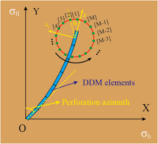
FIGURE 1. Division of fracture tip elements (Cong et al., 2021).

Fluid Flow Equation

Assuming that there is no relative slip on both sides of the fracture and the fluid pressure drop in the fracture is uniform, the Navier–Stokes equation can be simplified as

$\frac{dp}{dx}=\frac{12q\mu }{w^{3}h},(5)$

where p is the pressure in fracture, Pa; x is the fracture length, m; q is the injection rate, m³/min; μ is the fluid viscosity, mPa s; and w is the fracture width, w = D_n.

The material balance within the fracture can be written as

$\frac{\partial q\left(x,t\right)}{\partial x}-q_L\left(x,t\right)=\frac{\partial A\left(x,t\right)}{\partial t},(6)$

where q_L is the volume rate of fluid loss, m²/min; A is the cross-sectional area of the fracture, m².

When multiple fractures of horizontal wells propagate synchronously, the flow of fracturing fluid entering each fracture is different, but the total displacement of wellhead pumping is the sum of the displacement of each fracture cluster.

$Q_T={\displaystyle \sum _{i=1}^m{Q}_i},(7)$

According to Kirchoff’s second law, the pressure in the wellbore meets

$p_0=p_{w,i}+p_{f,i}+p_{cf,i}\left(i=\mathrm{1,2,3},\mathrm{...},m\right),(8)$

where p₀ is the total pressure at the wellbore heel, Pa; p_w,i is the fluid pressure at the inlet of fracture i, Pa; p_pf,i is the perforation friction of fracture i, Pa; and p_cf,i is the wellbore flow friction of fracture i, Pa。.

The perforation friction and wellbore flow friction can be calculated by Eqs 14, 15, respectively:

$p_{pf,i}=\frac{0.2369{\rho }_s}{n_{p,i}^2{d}_{p,i}^4{C}_{d,i}^2}{Q}_i^2,(9)$

where ρ_s is the density of the fracturing fluid, kg/m³; n_p,i is the number of perforations in fracture i; d_p,i is the perforation diameter of fracture i, m; and C_d,i is the correction factor of fracture i.

$p_{cf,i}=C_{cf}{\displaystyle \sum _{j=1}^i\left(x_j-x_{j-1}\right)Q_{w,j}},(10)$

where C_cf is the friction coefficient, Pa s/m⁴; x_j is the distance from fracture j to the horizontal wellbore heel, m; and Q_w,j is the remaining fluid flow after j fractures, m³/min.

Calculation Method of Leakage Volume Based on the Brinkman Equation

The fluid velocity at the interface between hydraulic fracture and rock is continuous, and there is a smooth velocity transition between the fracture area and porous rock area (Kahshan et al., 2020). Previously, Darcy’s law used to calculate the fluid loss volume was only applicable to describe the steady flow of fluid in porous media (He et al., 2021). In order to ensure that there is no velocity slip at the interface between rock and HF, the Brinkman equation is used to calculate the fluid velocity in rock. Combined with the fluid flow equation in fracture, the calculation method of fracturing fluid leakage velocity in different flow areas is constructed, as shown in Figure 2.

FIGURE 2

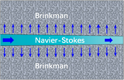
FIGURE 2. Brinkman–Stokes coupling filtration calculation schematic diagram.

The flow rate of fracturing fluid in the fracture is fast, and the flow rate in the rock matrix is relatively slow. The flow process is continuous at the interface of the two regions. Therefore, there is a region where the velocity increases significantly in the porous medium close to the fracture. To accurately describe the velocity distribution of fluid in this boundary layer, the Brinkman equation is used instead of the Darcy equation to calculate the flow velocity in the rock matrix (Martys et al., 1994).

$\frac{\mu }{K}{u}_{br}+\frac{dp}{dx}-\frac{\mu }{\varphi }\frac{d^2{u}_{br}}{d{y}^2}=0,(11)$

where K is the rock matrix permeability, m²; ϕ is the dimensionless porosity of the rock matrix; and u_br is the flow rate of the fracturing fluid in the rock matrix, m/s.

The Brinkman–Stokes coupling model needs to meet the following conditions: a) the flow velocity of the porous medium region and free flow region is continuous at the boundary; b) the shear stress at the boundary of the porous medium region and free flow region is continuous; and c) the fluid flow in the far area conforms to Darcy’s law.

$\{\begin{array}{l}\underset{y\to 0}{\lim }{u}_{br}=u_{ns}\\ \underset{y\to 0}{\lim }{\tau }_{br}={\tau }_{ns}\\ \underset{y\to \infty }{\lim }{u}_{br}=-\frac{K}{\mu }\frac{dp}{dy}=u_d\end{array},(12)$

where u_ns is the fluid velocity in the fracture, m/s; u_d is the leakage velocity obtained by Darcy’s law, m/s; τ_br and τ_ns are the fluid shear stress under the Brinkman equation and Stokes equation, respectively, which can be expressed as

$\begin{array}{cc}{\tau }_{ns}=\mu \frac{d{u}_{ns}}{dy},& {\tau }_{br}=\frac{\mu }{\varphi }\frac{d{u}_{br}}{dy}\end{array},(13)$

The leakage velocity of the fracturing fluid can be obtained by simultaneous Eqs 5, 11–13.

$u_{br}=\frac{u_{d}w\sqrt{\varphi }}{2\sqrt{K}}{e}^{\sqrt{\frac{\varphi }{Ky}}}+u_d,(14)$

The leakage rate be obtained by integral calculation along the direction of the rock matrix.

$q_L=2{\displaystyle \underset{0}{\overset{l}{\int }}{u}_{br}dy=u_{d}w\left(1-\exp \left(-\sqrt{\frac{\varphi }{K}l}\right)\right)},(15)$

where l is the thickness of the rock matrix, m.

Interaction Propagation Mechanism Between the HF and NF

Hydraulic fracturing of the shale oil reservoir can form complex fracture networks, and the most important reason is that the weak geological discontinuity represented by NF has a significant impact on HF propagation. If the HF does not directly penetrate the NF but turns to propagate along the NF surface, it is bound to increase the complexity of the HF network. When the HF approaches the NF (Figure 3), the induced stress at the tip of the HF is applied to the NF surface, causing changes in normal stress and shear stress.

FIGURE 3

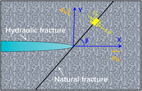
FIGURE 3. Schematic of the hydraulic fracture approaching the natural fracture.

Each stress in the tip area of the hydraulic crack is expressed as

$\{\begin{array}{l}{\sigma }_{xx}={\sigma }_{\text{H}}-\frac{K_{\mathrm{{\rm I}}}}{\sqrt{2\pi r}}\cos \frac{\theta }{2}\left(1-\sin \frac{\theta }{2}\sin \frac{3\theta }{2}\right)\\ {\sigma }_{yy}={\sigma }_{\text{h}}-\frac{K_{\mathrm{{\rm I}}}}{\sqrt{2\pi r}}\cos \frac{\theta }{2}\left(1+\sin \frac{\theta }{2}\sin \frac{3\theta }{2}\right)\\ {\sigma }_{xy}=-\frac{K_{\mathrm{{\rm I}}}}{\sqrt{2\pi r}}\sin \frac{\theta }{2}\cos \frac{\theta }{2}\cos \frac{3\theta }{2}\end{array},(16)$

where σ_H and σ_h are the maximum and minimum horizontal principal stress, respectively, Pa; K_Ⅰ is the stress intensity factor, Pa m^0.5。.

Two mechanical conditions need to be met for the HF to continue to propagate through the NF (Gu and Weng, 2010). One is that the maximum principal stress at the tip of the HF reaches the tensile strength of rock mass in the forward direction of the HF. The other is that there is no shear slip at the NF interface.

${\sigma }_1=T_0,(17)$

$\left|{\tau }_{\beta }\right|\le S_0+{\mu }_{\text{f}}{\sigma }_{n\beta },(\mathrm{18a})$

where σ₁ is the maximum principal stress, Pa; T₀ is the tensile strength of rock, Pa; τ_β is the shear stress on the wall of the NF, Pa; S₀ is the rock cohesion, Pa; μ_f is the friction coefficient; and σ_nβ is the normal stress on the wall of the NF, Pa.

Figure 4 is the interactive propagation chart of the HF and NF under different friction coefficients and stress conditions. When the approach angle β between the HF and NF is greater than 60°, with the increase in stress ratio, HFs are easier to penetrate the NF. Also, when the approach angle β is less than 60°, with the increase in stress ratio, HFs are easier to be captured by the NF. Under the same principal stress ratio, the greater the friction coefficient, the easier it is for the HF to penetrate the NF because under the condition of high friction coefficient, the greater the friction on the NF surface, the less likely it is to shear slip, which is conducive to the HF to directly pass through the NF surface. When the HF is 90° orthogonal to the NF, the friction coefficient is greater than 0.41, and the HF will hardly propagate along with the NF.

FIGURE 4

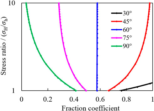
FIGURE 4. A crossing criterion for various intersection angles (Gu and Weng, 2010) (tensile strength T₀ = 0 and cohesion S₀ = 0). The region to the right of each curve is the crossing condition.

Numerical Method for the Model

The flow chart of the numerical algorithm is shown in Figure 5. First, rock, fluid, and other parameters are input, the initial fracture grid is constructed, and the initial fracture pressure P_i is assigned to each grid. The normal and shear displacements of each fracture element are calculated by Eqs 1, 2. ${\sigma }_n^i$ and ${\sigma }_s^i$ are determined by the remote and local stress boundary conditions, and the fracture width D_n of each DDM element is calculated by coordinate conversion. The flow rate and viscosity in each element are known; thus, the new pressure P_i+1 in the fracture is obtained according to Eq. 5. When the calculation error of P_i and P_i+1 is less than the convergence accuracy δ (δ = 0.001 MPa), the fracture propagation angle is calculated by the stress numerical search method (SNSM) (Cong et al., 2021), and a displacement discontinuous element is added in this direction (n is the convergence coefficient; in this article, n = 0.2). If the added unit meets the NF in the calculation domain, the interactive propagation is judged by the propagation criterion in Section 2.4. Otherwise, the HF will continue to propagate along the maximum circumferential stress direction until the fracturing operation is completed.

FIGURE 5

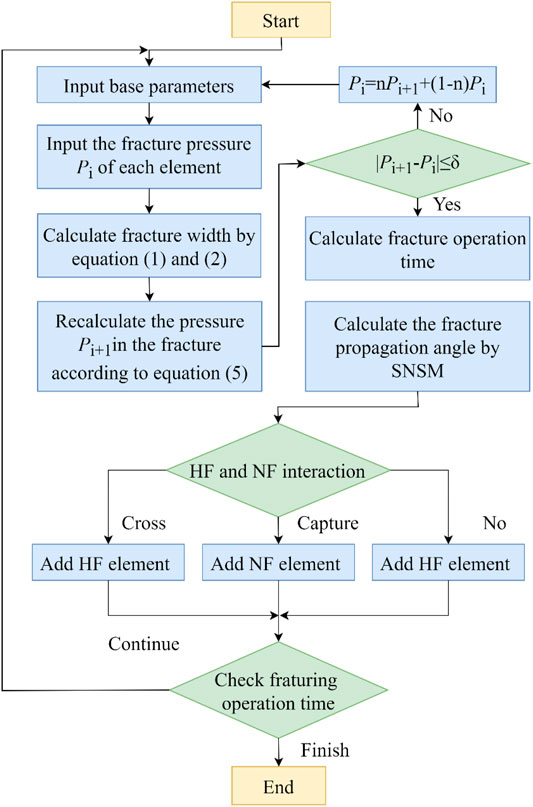
FIGURE 5. Flow chart of numerical algorithm.

When multiple fractures propagate, the fracture grows competitively under the action of “stress shadow” so that the fracture propagation length is different in each time step. Renshaw and Pollard (Renshaw and Pollard, 1994) proposed a multi-fracture growth step calculation method, which links the specific crack tip energy release rate G with the maximum crack tip energy release rate G_max in the calculation domain.

$\{\begin{array}{l}\begin{array}{cc}d{l}_i=0& G_i<G_c\end{array}\\ \begin{array}{cc}d{l}_i=d{l}_{\max }{\left(\frac{G_i}{G_{\max }}\right)}^{\varsigma }& G_i\ge G_c\end{array}\end{array},(\mathrm{18b})$

The energy release rate is the same as the J-integral value (Wu, 1978), which can be calculated according to the intensity factors K_Ⅰ and K_Ⅱ.

$G=\frac{K_{\mathrm{{\rm I}}}^2+K_{\mathrm{{\rm I}}\mathrm{{\rm I}}}^2}{E/\left(1-v^2\right)},(19)$

$K_{\mathrm{{\rm I}}}=\frac{0.806E\sqrt{\pi }}{4\left(1-{\nu }^2\right)\sqrt{2a}}{D}_n,(20)$

$K_{\mathrm{{\rm I}}\mathrm{{\rm I}}}=\frac{0.806E\sqrt{\pi }}{4\left(1-{\nu }^2\right)\sqrt{2a}}{D}_s,(21)$

where l is the increased crack element length, m; G is the energy release rate, N/m; ζ is an empirical parameter, which is taken as 1 in this paper; E is the modulus of elasticity, Pa; v is Poisson’s ratio; and a is the half length of the DDM element, m.

Model Validation

This work assumes that hydraulic fracture is a two-dimensional contour model, so the model in this article is compared with the KGD model, and the parameters required for calculation are shown in Table 1.

TABLE 1

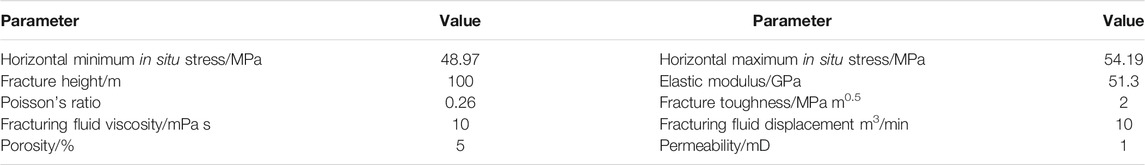
TABLE 1. Parameters for KGD model verification (Cheng, 2016).

Since the KGD model does not consider the influence of leakage on fracture propagation, the leakage term in Eq. 6 is ignored. Firstly, the model in this paper is used to calculate and compare the fracture width propagation without leakage, as shown in Figure 6. The calculation results show that when there is no leakage effect, the fracture width propagation curve of the KGD model and this model has high consistency. When the fracture propagates to 200 s, the fracture width calculated by the KGD model and this model is 4.13 and 4.32 mm, respectively, with a difference of only 4.3%. Considering the influence of fluid leakage, the crack width propagation is calculated by the Darcy equation and Brinkman equation, respectively. As part of the fracturing fluid leakage into the rock matrix, the fracture width values are lower than those in the non-leakage state, and the fracture width values obtained by the Brinkman equation are lower than the calculation results of the Darcy equation. The Darcy equation has a discontinuous velocity at the fracture boundary (as shown in Figure 7), while the Brinkman equation considers the continuous velocity of the fracturing fluid when it crosses the fracture boundary. The fracturing fluid flow rate shows a gentle downward trend, the calculated fracturing fluid filtration volume is more, and the fracturing fluid volume used for fracture propagation is reduced. Therefore, the results shown in Figure 6 appear.

FIGURE 6

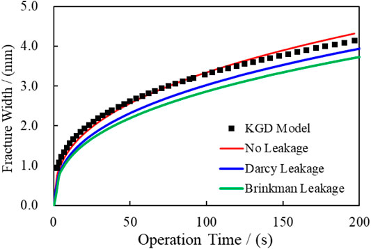
FIGURE 6. Comparison of fracture width.

FIGURE 7

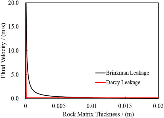
FIGURE 7. Comparison of the Brinkman model and Darcy model.

Wu and Olson (2014) systematically studied the propagation behavior of the HF after approaching the NF and well analyzed the interactive propagation behavior under different approaching angles, stress differences, crack lengths, and other factors. Two NFs (blue dotted line in Figure 8) are set on the HF propagation path. The propagation form of the HF is simulated by the model in this article and compared with the calculation results in the work of Wu and Olson (2014). The parameters are shown in Table 2, and the simulation results are shown in Figure 8B.

FIGURE 8

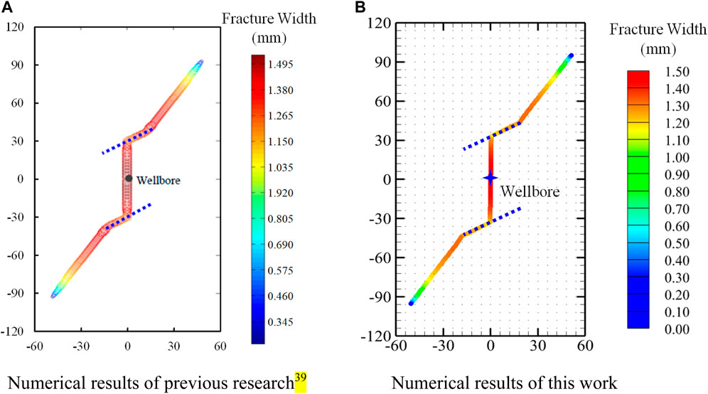
FIGURE 8. Comparison and verification of numerical simulation results. (A) Numerical results of previous research (Wu and Olson, 2014). (B) Numerical results of this work.

TABLE 2

TABLE 2. Basic data for HF and NF intersection (Wu and Olson, 2014).

The HF propagation results calculated by the model in this article are basically consistent with the existing simulation results. When the HF approaches the NF, the HF cannot penetrate the NF. After extending to the end of the NF, the HF continues to propagate in the rock matrix at a certain angle. At the intersection of the HF and NF, the fracture width has an obvious downward trend. In the literature, the fracture width at the injection point is 1.495 mm, and that of the model in this article is 1.443 mm. When the end of the NF extends to the rock matrix, the included angles between the HF and the X-direction are 59° and 61°, respectively. The comparison results show that the calculation results of the two models are in good agreement, which proves that the fracture propagation model in this paper has good accuracy in characterizing the interactive propagation of the HF and NF.

Calculation and Results

The geological parameters of the second member of Kongdian Formation on the Cangdong Depression area and the construction parameters of G 1701H well (Table 3) (Zhao et al., 2018a; Zhao et al., 2018b; Zhao et al., 2020) are used to calculate the fracture propagation under different interaction modes of the HF and NF. The design vertical depth of G1701H is 3,848.98 m, and the horizontal section is 1,503.87 m long, along the east–west direction (Figure 9). The orientation of the maximum horizontal principal stress in the second member of Kongdian Formation is north–west 30°.

TABLE 3

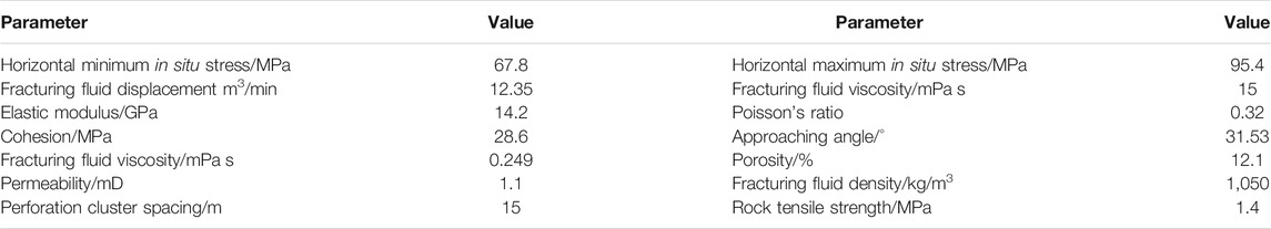
TABLE 3. Basic data of the second member of Kongdian Formation and G1701H (Zhao et al., 2018a; Zhao et al., 2018b; Zhao et al., 2020).

FIGURE 9

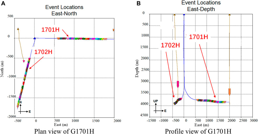
FIGURE 9. Layout of G1701H Well. (A) Plan view of G1701H. (B) Profile view of G1701H.

Case A: HF Propagation Without NF

We calculated the propagation of the HF without the NF, as shown in Figure 10. Due to the certain deflection between the direction of formation principal stress and the coordinate axis, the three horizontally arranged perforation clusters do not propagate perpendicular to the X-axis but extend along the direction of the maximum horizontal principal stress. Relevant research (Li et al., 2014; Wang et al., 2016) shows that the larger the horizontal stress difference is, the lower the deflection caused by “stress shadow” is and the more obvious the phenomenon of uneven fracture growth is. The horizontal stress difference in the study area is close to 30 MPa, the three HFs basically propagate in a straight line, and the growth of the middle HF is obviously restrained. At the end of the calculation, the length of HFs on both sides is close to 100 m, and the middle is only 70 m. Comparing the numerical simulation results with the on-site microseismic monitoring results, it is found that case A matches well with stage 6 of G1701H (Figure 11). The number of microseismic events in this stage is only 1,404, which is at a low level in fracturing stage 13 of the whole well. Combined with the direction of horizontal principal stress, it can be inferred that, during the fracturing of stage 6, the HF only opened the rock matrix and formed a simple fracture shape, and the HF propagation area did not intersect with the natural fracture zone.

FIGURE 10

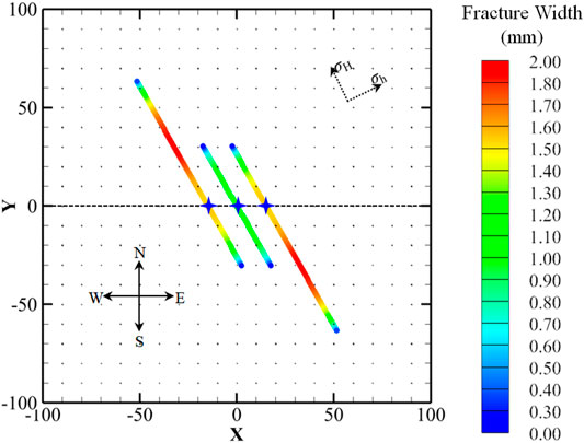
FIGURE 10. Numerical results of case A.

FIGURE 11

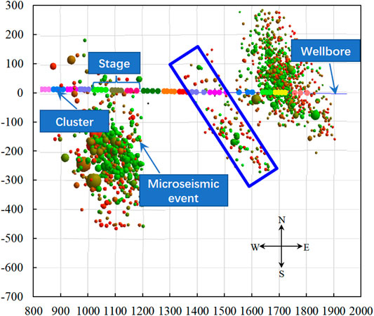
FIGURE 11. Microseismic detection results of G1701H at stage 6.

Case B: HF Propagation With Full NF

The NF zone along the direction of minimum horizontal principal stress is set to pass through the horizontal wellbore. The length of each fracture in the NF zone is 36 m, the spacing of fractures in the X-direction is 4 m, and the spacing of fractures in the Y-direction is 5 m. The simulation results are shown in Figure 12. Since the HF cannot meet the mechanical conditions of penetrating the NF, when it approaches the NF, the HF is captured by the NF and propagates along with it. After reaching the end of the NF, the HF enters the rock matrix and propagates until it is captured by the next NF. It can also be seen in Figure 12 that although the NF existence changes the complexity of HF, the length of the fracture in the middle is still significantly shorter than that on both sides under the action of “stress shadow.” Compared with the microseismic monitoring results of G1701H well, it is found that the simulation results are highly consistent with those of stage 4. The number of microseismic events in this stage is 2,566, and the microseismic events basically occur near the left and right clusters of fractures and then extend to the north–east, indicating that the NF in the fracturing area of stage 4 is relatively developed (Figure 13). During the propagation process, a large number of NFs along the minimum horizontal principal stress are activated, forming a more complex fracture network.

FIGURE 12

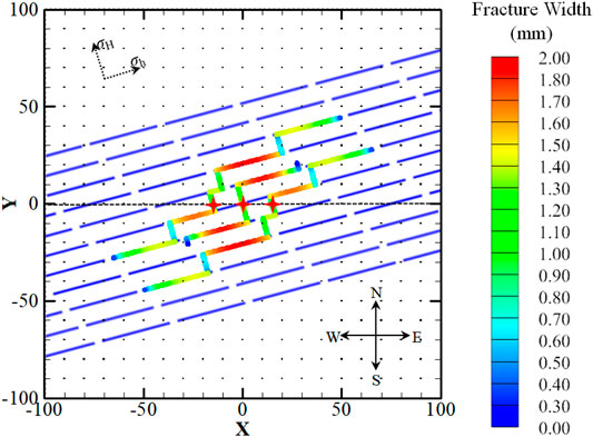
FIGURE 12. Numerical results of case B.

FIGURE 13

FIGURE 13. Microseismic detection results of G1701H at stage 4.

Case C: HF Propagation With Half NF

Figure 14 shows the results of HF propagation when the NF zone is only located in the part of the perforation cluster area. Since the left and middle HFs do not contact the NF, the fractures propagate in a straight line along the maximum horizontal principal stress direction. After the right fracture is captured by the NF, the distance between the north wing and the middle HF gradually increases, while the distance between the south wing and the middle HF decreases, which changes the “stress shadow” effect, making the north and south wings of the middle crack grow asymmetrically. The microseismic monitoring results shown in Figure 15 were obtained from stage 2 of G 1701H Well. The number of fracturing microseismic events in this stage is 1855. Double fractures appear. The main fracture direction is northeast-southwest, and the fractures extend more in the northeast direction. It can also be seen that the branch fractures in the northwest–southeast direction have a short extension distance compared with the main fracture. Combined with the simulation results in Figure 14, it can be inferred that the perforation cluster on the left side of the HF intersects with the NF zone, forming the main fracture along the direction of the minimum horizontal principal stress, while the right fracture without passing through the NF zone continues to propagate in the rock matrix and finally forms a “T”-shaped fracture network.

FIGURE 14

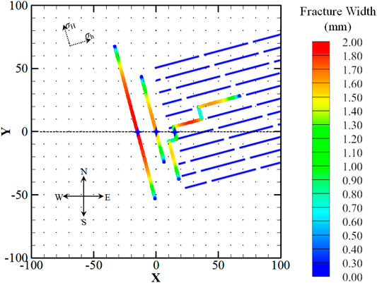
FIGURE 14. Numerical results of case C.

FIGURE 15

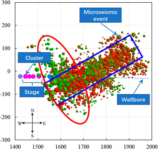
FIGURE 15. Microseismic detection results of G1701H at stage 2.

Discussion

In this work, the Brinkman equation is used to modify the existing leakage model based on Darcy’s law, and combined with the DDM method, the fracture propagation law under different interaction modes of HF and NF is simulated. Since there is a velocity transition region between the HF region and the porous rock matrix region, the Brinkman equation considering the velocity drop in the transition region is more in line with the real flow in fractures and rocks. Comparing Darcy’s law with Eq. 14, it is found that there is an additional velocity term in the leakage rate model in this paper, which is the impact on fracturing fluid leakage in the transition region. According to the generalized Darcy law, the equivalent permeability of the rock matrix in the presence of a transition area is

$K^{\prime }=\frac{q_L+q_L^{\prime }}{q_L}K=\left(1+\frac{6w\left(\sqrt{\varphi }w+2\sqrt{K}\right)}{w^2\sqrt{K}}\right)K,(22)$

We set

$\psi =\frac{6w(\sqrt{\varphi }w+2\sqrt{K})}{w^2\sqrt{K}},(23)$

where ψ indicates the influence of the transition region on the equivalent permeability of the rock matrix. It can be seen from Figure 16 that, under the premise of certain porosity, with the increase in fracture width, the influence of the transition area on rock equivalent permeability becomes greater. The greater the matrix permeability, the more the fracturing fluid will enter the rock through the transition area, and the ψ value is larger (Figure 17). Reducing porosity indicates that the proportion of rock in porous media increases, which reduces the possibility of fracturing fluid entering the rock matrix, and the impact of fracturing fluid flow rate drop on filtration in the transition zone will gradually decrease.

FIGURE 16

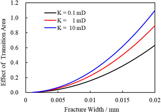
FIGURE 16. Effect of permeability on equivalent permeability.

FIGURE 17

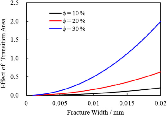
FIGURE 17. Effect of porosity on equivalent permeability.

In this work, a new model is used to simulate the propagation of HF in three cases: perforation clusters without NF, in NF zones, and some perforation clusters in NF zones. At the same time, combined with microseismic monitoring data, the real propagation of formation fractures is explained. The research shows that the NF zone will change the propagation direction of the main fracture. The more complex the fracture is, the more the number of microseismic monitoring events is. When only some HFs meet natural fractures, a “T”-shaped fracture network may be formed.

The model and simulation method can be well used for fracturing simulation of the shale oil reservoir and can provide references for fracturing parameter design, fracture parameter inversion, and other related fields. However, this model also has some shortcomings, such as the single NF length and angle set in the model, and the influence of formation rock thermal stress on fracture propagation is not considered. Further research is still needed to further improve this model.

Conclusion

1) There is a flow velocity transition region between the HF wall and porous rock matrix. The flow velocity change can be accurately calculated by the Brinkman equation, and the calculated leakage volume is larger than the Darcy equation.

2) The influence of the transition region on leakage is related to rock porosity and permeability parameters. The greater the porosity and permeability of the rock matrix, the greater the influence of the transition region on filtration.

3) Under high stress difference, when multiple cluster fractures crack synchronously, each HF will hardly deflect, but the middle fracture propagation is obviously restrained.

4) The NF zone will change the propagation direction of the main fracture. When there are multiple clusters of fractures in the same stage, only some HFs meet the NF, and it is easy to form a “T”-shaped fracture network.

Data Availability Statement

The original contributions presented in the study are included in the article/Supplementary Material, further inquiries can be directed to the corresponding author.

Author Contributions

Conceptualization: YL; methodology: FT and YL; investigation: YL; writing—original draft preparation: FT; and writing—review and editing: YJ, LS, and ZC.

Funding

The research was supported by the National Natural Science Foundation of China (No. 52174024).

Conflict of Interest

Author FT is employed by Dagang Oilfield of CNPC.

The remaining authors declare that the research was conducted in the absence of any commercial or financial relationships that could be construed as a potential conflict of interest.

Publisher’s Note

All claims expressed in this article are solely those of the authors and do not necessarily represent those of their affiliated organizations, or those of the publisher, the editors, and the reviewers. Any product that may be evaluated in this article, or claim that may be made by its manufacturer, is not guaranteed or endorsed by the publisher.

References

Bakhshi, E., Rasouli, V., Ghorbani, A., Marji, M. F., Damjanac, B., and Wan, X. (2019). Lattice Numerical Simulations of Lab-Scale Hydraulic Fracture and Natural Interface Interaction. Rock Mech. Rock Eng. 52 (5), 1315–1337. doi:10.1007/s00603-018-1671-2

CrossRef Full Text | Google Scholar

Cai, W., Dou, L., Zhang, M., Cao, W., Shi, J.-Q., and Feng, L. (2018). A Fuzzy Comprehensive Evaluation Methodology for Rock Burst Forecasting Using Microseismic Monitoring. Tunnelling Underground Space Technol. 80, 232–245. doi:10.1016/j.tust.2018.06.029

CrossRef Full Text | Google Scholar

Cheng, W., Jiang, G. S., Xie, J. Y., Wei, Z. J., and Li, X. D. (2019). A Simulation Study Comparing the Texas Two-step and the Multistage Consecutive Fracturing Method. Pet. Sci. 1. doi:10.1007/s12182-019-0323-9

CrossRef Full Text | Google Scholar

Cheng, W. (2016). Mechanism of Hydraulic Fracture Propagation in Fractured Shale Reservoir in Three Dimensional Space. China, Beijing: China University of Petroleum.

Google Scholar

Cong, Z., Li, Y., Liu, Y., and Xiao, Y. (2021). A New Method for Calculating the Direction of Fracture Propagation by Stress Numerical Search Based on the Displacement Discontinuity Method. Comput. Geotechnics 140, 104482. doi:10.1016/j.compgeo.2021.104482

CrossRef Full Text | Google Scholar

Cong, Z., Li, Y., Pan, Y., Liu, B., Shi, Y., Wei, J., et al. (2022). Study on CO 2 Foam Fracturing Model and Fracture Propagation Simulation. Energy 238 (238), 121778. doi:10.1016/j.energy.2021.121778

CrossRef Full Text | Google Scholar

Dong, J., Chen, M., Li, Y., Wang, S., Zeng, C., and Zaman, M. (2019). Experimental and Theoretical Study on Dynamic Hydraulic Fracture. Energies 12 (3), 397. doi:10.3390/en12030397

CrossRef Full Text | Google Scholar

Fu, P. C., Johnson, S. M., and Carrigan, C. R. (2013). An Explicitly Coupled Hydro-Geomechanical Model for Simulating Hydraulic Fracturing in Arbitrary Discrete Fracture Networks. Int. J. Numer. Anal. Methods Geomechanics 37 (14), 2278–2300. doi:10.1002/nag.2135

CrossRef Full Text | Google Scholar

Fu, W., Savitski, A. A., Damjanac, B., and Bunger, A. P. (2018). Three-dimensional Lattice Simulation of Hydraulic Fracture Interaction with Natural Fractures. Comput. Geotechnics 107, 214–234.

Google Scholar

Gao, R., Kuang, T., Zhang, Y., Zhang, W., and Quan, C. (2021). Controlling Mine Pressure by Subjecting High-Level Hard Rock Strata to Ground Fracturing. Int. J. Coal Sci. Technol. 8 (6), 1336–1350. doi:10.1007/s40789-020-00405-1

CrossRef Full Text | Google Scholar

Gottardi, R., and Mason, S. L. (2018). Characterization of the Natural Fracture System of the eagle ford Formation (Val Verde County, Texas). AAPG Bull. 102 (10), 1963–1984. doi:10.1306/03151817323

CrossRef Full Text | Google Scholar

Gu, H., and Weng, X. In Criterion for Fractures Crossing Frictional Interfaces at Non-orthogonal Angles, Salt Lake City: Us Rock Mechanics Symposium & Us-canada Rock Mechanics Symposium, 2010.

Google Scholar

Guo, J. C., Luo, B., Lu, C., Lai, J., and Ren, J. C. (2017). Numerical Investigation of Hydraulic Fracture Propagation in a Layered Reservoir Using the Cohesive Zone Method. Eng. Fracture Mech. 186, 195–207. doi:10.1016/j.engfracmech.2017.10.013

CrossRef Full Text | Google Scholar

He, X., Alsinan, M., Kwak, H., and Hoteit, H. (2021). “High-Resolution Micro-continuum Approach to Model Matrix-Fracture Interaction and Fluid Leakage,”in SPE Middle East Oil & Gas Show and Conference, November 2021. Manama: OnePetro. doi:10.2118/204531-ms

CrossRef Full Text | Google Scholar

Kahshan, M., Lu, D., Abu-Hamdeh, N. H., Golmohammadzadeh, A., Farooq, A., and Rahimi-Gorji, M. (2020). Darcy-Brinkman Flow of a Viscous Fluid through a Porous Duct: Application in Blood Filtration Process. J. Taiwan Inst. Chem. Eng. 117, 223–230. doi:10.1016/j.jtice.2020.11.033

CrossRef Full Text | Google Scholar

Ladevèze, P., Rivard, C., Lavoie, D., Séjourné, S., Lefebvre, R., and Bordeleau, G. (2019). Fault and Natural Fracture Control on Upward Fluid Migration: Insights from a Shale Gas Play in the St. Lawrence Platform, Canada. Hydrogeology J. 27 (1), 121–143.

Google Scholar

Lan, Z., and Gong, B. (2020). Uncertainty Analysis of Key Factors Affecting Fracture Height Based on Box-Behnken Method. Eng. Fracture Mech. 228 (11), 106902. doi:10.1016/j.engfracmech.2020.106902

CrossRef Full Text | Google Scholar

Lecampion, B. (2009). An Extended Finite Element Method for Hydraulic Fracture Problems. Commun. Numer. Methods Eng. 25 (2), 121–133. doi:10.1002/cnm.1111

CrossRef Full Text | Google Scholar

Li, D. Q., Zhang, S., and Zhang, S. A. (2014). Experimental and Numerical Simulation Study on Fracturing through Interlayer to Coal Seam. J. Nat. Gas Sci. Eng. 21, 386–396. doi:10.1016/j.jngse.2014.08.022

CrossRef Full Text | Google Scholar

Li, Y., Jia, D., Wang, M., Liu, J., Fu, C., Yang, X., et al. (2016). Hydraulic Fracturing Model Featuring Initiation beyond the Wellbore wall for Directional Well in Coal Bed. J. Geophys. Eng. 168 (4), 536–548. doi:10.1088/1742-2132/13/4/536

CrossRef Full Text | Google Scholar

Li, Y., Long, M., Tang, J., Chen, M., and Fu, X. (2020). A Hydraulic Fracture Height Mathematical Model Considering the Influence of Plastic Region at Fracture Tip. Pet. Exploration Develop. 47 (1), 184–195. doi:10.1016/s1876-3804(20)60017-9

CrossRef Full Text | Google Scholar

Li, Y., and Weijermars, R. (2019). Wellbore Stability Analysis in Transverse Isotropic Shales with Anisotropic Failure Criteria. J. Pet. Sci. Eng. 176, 982–993. doi:10.1016/j.petrol.2019.01.092

CrossRef Full Text | Google Scholar

Li, Y. W., Long, M., Zuo, L. H., Li, W., and Zhao, W. C. (2019). Brittleness Evaluation of Coal Based on Statistical Damage and Energy Evolution Theory. J. Pet. Sci. Eng. 172, 753–763. doi:10.1016/j.petrol.2018.08.069

CrossRef Full Text | Google Scholar

Li, Y., Zhao, Y., Tang, J., Zhang, L., Zhou, Y., Zhu, X., et al. (2020). Rock Damage Evolution Model of Pulsating Fracturing Based on Energy Evolution Theory. Energ. Sci. Eng. 8 (4), 1050–1067. doi:10.1002/ese3.567

CrossRef Full Text | Google Scholar

Liang, Z., Xue, R., Xu, N., and Li, W. (2020). Characterizing Rockbursts and Analysis on Frequency-Spectrum Evolutionary Law of Rockburst Precursor Based on Microseismic Monitoring. Tunnelling Underground Space Technol. 105, 103564. doi:10.1016/j.tust.2020.103564

CrossRef Full Text | Google Scholar

Liu, X., Qu, Z., Guo, T., Sun, Y., Wang, Z., and Bakhshi, E. (2019). Numerical Simulation of Non-planar Fracture Propagation in Multi-Cluster Fracturing with Natural Fractures Based on Lattice Methods. Eng. Fracture Mech. 220, 106625. doi:10.1016/j.engfracmech.2019.106625

CrossRef Full Text | Google Scholar

Martys, N., Bentz, D. P., and Garboczi, E. J. (1994). Computer Simulation Study of the Effective Viscosity in Brinkman's Equation. Phys. Fluids 6 (4), 1434–1439. doi:10.1063/1.868258

CrossRef Full Text | Google Scholar

Olson, J. E. (2004). Predicting Fracture Swarms—The Influence of Subcritical Crack Growth and the Crack-Tip Process Zone on Joint Spacing in Rock. Geol. Soc. Lond. Spec. Publications 231 (1), 73–88. doi:10.1144/gsl.sp.2004.231.01.05

CrossRef Full Text | Google Scholar

Olson, J. (1989). Inferring Paleostresses from Natural Fracture Patterns: A New Method. Geology 17 (4), 345–348. doi:10.1130/0091-7613(1989)017<0345:ipfnfp>2.3.co;2

CrossRef Full Text | Google Scholar

Renshaw, C. E., and Pollard, D. D. (1994). Numerical Simulation of Fracture Set Formation: A Fracture Mechanics Model Consistent with Experimental Observations. J. Geophys. Res. Solid Earth 99 (B5), 9359–9372. doi:10.1029/94jb00139

CrossRef Full Text | Google Scholar

Sih, G. C. (1974). Strain Energy Density Factor Applied to Mixed Mode Crack Problems. Int. J. Fracture 10 (3), 305–321. doi:10.1007/bf00035493

CrossRef Full Text | Google Scholar

Tang, J. Z., and Wu, K. (2018). A 3-D Model for Simulation of Weak Interface Slippage for Fracture Height Containment in Shale Reservoirs. Int. J. Sol. Structures 144, 248–264. doi:10.1016/j.ijsolstr.2018.05.007

CrossRef Full Text | Google Scholar

Tang, J. Z., Wu, K., Zeng, B., Huang, H. Y., Hu, X. D., Guo, X. Y., et al. (2018). Investigate Effects of Weak Bedding Interfaces on Fracture Geometry in Unconventional Reservoirs. J. Pet. Sci. Eng. 165, 992–1009. doi:10.1016/j.petrol.2017.11.037

CrossRef Full Text | Google Scholar

Wang, J., Yang, J., Wu, F., Hu, T., and Faisal, S. A. (2020). Analysis of Fracture Mechanism for Surrounding Rock Hole Based on Water-Filled Blasting. Int. J. Coal Sci. Technol. 7 (4), 704–713. doi:10.1007/s40789-020-00327-y

CrossRef Full Text | Google Scholar

Wang, X. L., Liu, C., Wang, H., Liu, H., and Wu, H. A. (2016). Comparison of Consecutive and Alternate Hydraulic Fracturing in Horizontal wells Using XFEM-Based Cohesive Zone Method. J. Pet. Sci. Eng. 143, 14–25. doi:10.1016/j.petrol.2016.02.014

CrossRef Full Text | Google Scholar

Weng, X., Kresse, O., Cohen, C., Wu, R., and Gu, H. (2011). Modeling of Hydraulic-Fracture-Network Propagation in a Naturally Fractured Formation. Spe Prod. Operations 26 (4), 368–380. doi:10.2118/140253-pa

CrossRef Full Text | Google Scholar

Wu, C. H. (1978). Fracture under Combined Loads by Maximum-Energy-Release-Rate Criterion. J. Appl. Mech. 45 (3), 553–538. doi:10.1115/1.3424360

CrossRef Full Text | Google Scholar

Wu, K., and Olson, J. E. (2014). “Mechanics Analysis of Interaction between Hydraulic and Natural Fractures in Shale Reservoirs,”in Unconventional Resources Technology Conference, .doi:10.15530/urtec-2014-1922946

CrossRef Full Text | Google Scholar

Wu, K., and Olson, J. E. (2015). Simultaneous Multifracture Treatments: Fully Coupled Fluid Flow and Fracture Mechanics for Horizontal Wells. Spe J. 20 (2), 337–346. doi:10.2118/167626-pa

CrossRef Full Text | Google Scholar

Xue, J., Wang, H., Zhou, W., Ren, B., Duan, C., and Deng, D. (2015). Experimental Research on Overlying Strata Movement and Fracture Evolution in Pillarless Stress-Relief Mining. Int. J. Coal Sci. Technol. 2 (1), 38–45. doi:10.1007/s40789-015-0067-0

CrossRef Full Text | Google Scholar

Zeng, Q., and Yao, J. (2016). Numerical Simulation of Fracture Network Generation in Naturally Fractured Reservoirs. J. Nat. Gas Sci. Eng. 30, 430–443. doi:10.1016/j.jngse.2016.02.047

CrossRef Full Text | Google Scholar

Zhang, F., Damjanac, B., and Maxwell, S. (2019). Investigating Hydraulic Fracturing Complexity in Naturally Fractured Rock Masses Using Fully Coupled Multiscale Numerical Modeling. Rock Mech. Rock Eng. 52 (12), 5137–5160. doi:10.1007/s00603-019-01851-3

CrossRef Full Text | Google Scholar

Zhang, F., Wang, X., Tang, M., Du, X., and Damjanac, B. (2021). Numerical Investigation on Hydraulic Fracturing of Extreme Limited Entry Perforating in Plug-And-Perforation Completion of Shale Oil Reservoir in Changqing Oilfield, China. Rock Mech. Rock Eng. 54 (6). doi:10.1007/s00603-021-02450-x

CrossRef Full Text | Google Scholar

Zhang, J., Li, Y., Pan, Y., Wang, X., Yan, M., Shi, X., et al. (2021). Experiments and Analysis on the Influence of Multiple Closed Cemented Natural Fractures on Hydraulic Fracture Propagation in a Tight sandstone Reservoir. Eng. Geology. 281, 105981. doi:10.1016/j.enggeo.2020.105981

CrossRef Full Text | Google Scholar

Zhao, X., Yang, F., Zhou, L., Xiugang, P. U., Jin, F., Han, W., et al. (2018). Geological Characteristics of Shale Rock System and Shale Oil Exploration Breakthrough in a Lacustrine basin: A Case Study from the Paleogene 1st Sub-member of Kong 2 Member in Cangdong Sag, Bohai Bay Basin, China. Pet. Exploration Develop. 45 (03), 377–388. doi:10.1016/s1876-3804(18)30043-0

CrossRef Full Text | Google Scholar

Zhao, X., Zhou, L., Xiugang, P. U., Jin, F., Jiang, W., Xiao, D., et al. (2018). Development and Exploration Practice of the Concept of Hydrocarbon Accumulation in Rifted-basin Troughs: A Case Study of Paleogene Kongdian Formation in Cangdong Sag, Bohai Bay Basin. Pet. Exploration Develop. 45 (6), 1092–1102. doi:10.1016/s1876-3804(18)30120-4

CrossRef Full Text | Google Scholar

Zhao, X., Zhou, L., Xiugang, P. U., Jin, F., and Jianying, M. A. (2020). Formation Conditions and Enrichment Model of Retained Petroleum in Lacustrine Shale: A Case Study of the Paleogene in Huanghua Depression, Bohai Bay Basin, China. Pet. Exploration Develop. 47 (5), 916–930. doi:10.1016/s1876-3804(20)60106-9

CrossRef Full Text | Google Scholar