- 1National Space Science Center, Chinese Academy of Sciences, Beijing, China
- 2University of Chinese Academy of Sciences, Beijing, China
- 3DFH Satellite Co. Ltd., Beijing, China
- 4Space Research Institute, Austrian Academy of Sciences, Graz, Austria
- 5National Institute of Natural Hazards, Ministry of Emergency Management of China, Beijing, China
- 6Institute of Experimental Physics, Graz University of Technology, Graz, Austria
Based on the in-orbit magnetic field data of the China Seismo-Electromagnetic Satellite (CSES) and Swarm satellites, some research studies on the data consistency cross comparison were carried out. The condition applied is that two satellites pass by in a relatively short period of time and through the spatial location at a relatively close range, and different spatial-temporal scale standards were set, combined with the Kp index to screen for geomagnetic quiet periods. Then, with the help of the CHAOS model, indirect analysis was realized. Furthermore, the difference between the in-orbit data and model value was visualized, and the phenomenon and possible reason for data variation with time and geomagnetic latitude variation were analyzed. These analysis results are displayed in this study, which may evaluate the reliability of the satellite magnetic field detection data and the consistency of multiple satellite detection results and provide a methodological reference for carrying out similar evaluation and analysis subsequently.
1 Introduction
The China Seismo-Electromagnetic Satellite (CSES), also called ZHANGHENG-1, was successfully launched from Jiuquan Satellite Launch Center on 2 February 2018 and started in-orbit operation on 5 February 2018. CSES is the first satellite in China to provide space-based data for earthquake observation and geomagnetic field measurement (Shen et al., 2018). The High Precision Magnetometer (HPM) onboard CSES comprises two fluxgate magnetometers (FGMs) and the Coupled Dark State Magnetometer (CDSM), which is developed by the National Space Science Center, Chinese Academy of Sciences in cooperation with the Space Research Institute, Austrian Academy of Sciences and the Institute of Experimental Physics, Graz University of Technology (Cheng et al., 2015). The CDSM measures the magnitude of the field with higher accuracy and stability, thus being used to ensure the accuracy of the vector magnetic field measurement in orbit (Cheng et al., 2018). The satellite is in a sun-synchronous orbit with an altitude of approximately 507 km and an inclination angle of 97.4°. The descending node of the CSES is at around 14:00 in local time, and the revisiting period is 5 days. The distance between adjacent orbits is about 2,650 km in 1 day and 530 km in the 5-day revisiting (Shen et al., 2018).
The Swarm satellites were successfully launched into orbit on 22 November 2013. The mission consists of three identical satellites Alpha, Bravo, and Charlie. On 17 April 2014, they formed a constellation to observe and study the Earth’s magnetic field. Each satellite carries an Absolute Scalar Magnetometer (ASM) measuring scalar magnetic field intensity and a Vector Fluxgate Magnetometer (VFM) measuring vector components. The ASM was designed by Laboratoire d'électronique des technologies de l’information, Commissariat à l'énergie atomique et aux énergies alternatives (CEA-Leti) in Grenoble and developed in close partnership with Centre National d'Etudes Spatiales (CNES), with scientific support from Institut de physique du globe de Paris (IPGP). It has the characteristic of being capable of continuously measuring both scalar and vector data at the same time, benefiting from its innovative design (Fratter et al., 2016). Alpha and Charlie satellites started their missions at an altitude of about 462 km, flying almost side by side in a near-polar orbit with an inclination of 87.35°. Bravo has an altitude of about 511 km and an inclination angle of about 87.75°. According to the mission design, the orbital planes of the three satellites drift slowly in local time, with a drifting rate of 2.74 h per month for Alpha and Charlie and a drifting rate of 2.61 h for Bravo (Olsen and Floberghagen, 2018).
The cross comparison and validation between satellites is an effective means of space exploration, which is of great significance to the data processing algorithm and data product quality in space exploration. At present, CSES and Swarm satellites are operating well in orbit and have obtained high-quality space magnetic field data in accordance with their own specifications for a long period of time. The two satellite missions are in orbit at the same time and have similar altitudes, and they have the same type of observation payloads (scalar magnetometer), which can be selected to carry out cross-study of magnetic field data. According to the satellite orbit characteristics, CSES and Swarm satellites have different orbital heights and inclination angles, so they cannot achieve long-term orbital overlapping flight and do not have the conditions to carry out direct data cross comparison. So, the data screening method and cross comparison method were applied to realize an indirect comparison analysis between the CSES and Swarm scalar magnetic field data.
The CHAOS-7 model describes the near-Earth geomagnetic field based on observations collected by satellites including Swarm, CryoSat-2, CHAMP, SAC-C, and Ørsted (Finlay et al., 2020). Only the data from dark regions (Sun elevation angle 10° below the horizon) were used to reduce the influence of ionospheric currents, and more detailed information about the CHAOS model can be obtained from the study by Olsen et al. (2006). As a reference field model, CHAOS can relate the magnetic vector, at the location and time of measurement, to the geographic directions (Finlay et al., 2020). So, the model can be taken advantage of to assist the cross comparison research.
2 Cross Comparison Methods
On the basis of the research objective, several steps are required during the data processing and analysis, including data screening methods with different criteria, cross comparison by virtue of the CHAOS-7.8 model, and methods of analysis.
2.1 Data Screening Methods
The CDSM data of CSES were derived from the scalar magnetic field level 2 data of HPM from the official website of the Center of Satellite Application in Earthquake Science, with a sampling frequency of 1 Hz and a time range from 2019 to 2020. The ASM data of Swarm Bravo were acquired from the 1 Hz sampling frequency L1b data product published on the official website of the European Space Agency, with a file version of 0505 and 0506, covering a period of time from 2019 to 2020. The Kp index was obtained from the page of GeoForschungsZentrum (GFZ) Potsdam (Matzka et al., 2021).
Some comparison conditions were set up in previous studies. The comparison between scalar measurements from the different satellites of Swarm was carried out for the data on 21 December 2013 which was magnetically quiet, and for each position of Alpha, the nearest Bravo and Charlie positions were selected for spatial co-localization (Fratter et al., 2016). The CSES and Swarm data for the period from August 30 to 3 September 2018 when the geomagnetic field was relatively quiet were chosen to perform a comparison (Zhou et al., 2019). Data for the time interval from November 15 to 30, 2018 were selected for comparison as the local time ranges overlapped for the CSES and Swarm Bravo night-side orbits (Pollinger et al., 2020). In this study, the condition was applied that two satellites pass by in a relatively short period of time and through the spatial location at a relatively close range, which means that the differences in UTC time and geographic longitude and latitude are small. As it was considered that the time and spatial difference may have an influence on the comparison results, it is necessary to choose an appropriate spatial–temporal scale standard. So, the term “time interval” was defined as the UTC time difference between the CDSM and ASM, and the term “spatial distance” as geographic longitude and latitude differences between the CDSM and ASM. The difference of altitude was taken into account by the application of the CHAOS model and precise calculation. To figure out whether the standards had an influence on the final results, several spatial–temporal scales were set up.
Applying the same analysis process, the influence of different scales would be further evaluated. A time interval of 30 min and spatial distance ranging from 1° × 1° to 20° x 20° in longitude and latitude can be compared to assess the influence of spatial scale. Meanwhile, spatial distance of 10°×10° and different time intervals can be compared to assess the influence of the time scale. Also, the dataset size on different spatial–temporal scales would be focused on and elaborated.
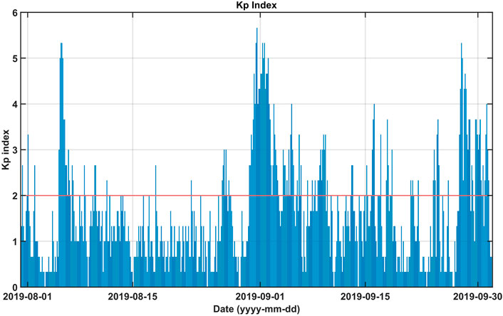
It is thought to be proper to apply a certain constraint that the time interval was set to be 180 min, and the spatial distance was set to be 5° × 5°. The results of other scales and periods will be discussed together later. Moreover, in consideration of geomagnetic field activities, the time periods when the Kp index is lower than 2+ were selected to screen for geomagnetic activity quiet periods (Yang et al., 2021). Other restrictions included Flags_F of ASM is 0 or 1, FLAG_MT of CDSM is 0, and parameter A211 should not be −9999.0. Flags_F of ASM characterizes the magnetic field intensity measurement. When its value is 0, the ASM works in scalar mode, and value 1 means the ASM running in vector mode. Both the values can ensure that ASM data is available for normal measurement, while other values represent some abnormal situations (National Space Institute Technical University of Denmark, 2019). For more details about the data product definition, product data handbooks are available released by the European Space Agency (see https://earth.esa.int/eogateway/missions/swarm/product-data-handbook). FLAG_MT of CDSM characterizes the disturbance of magnetic torque. When the magnetic torque is working, usually in high-latitude regions or near the equator, there is interference and the value is 1; otherwise, the value is 0. A211 is the scalar magnetic field intensity, and the value −9999.0 means invalid data (National Institute of Natural Hazards Ministry of Emergency Management of China, 2020).
To begin with, data from August to September 2019 was selected to perform a preliminary analysis, and the detailed process and results will be elaborated on. After this data screening process, suitable data were selected and distributed on some of the orbits of dates from 31 July 2019 to 30 September 2019. The dataset size is 550604 of CDSM day-side data, 546082 of CDSM night-side data, 713315 of ASM day-side data, and 658684 of ASM night-side data.
Figure 1 shows all the Kp indexes during this period, and the data corresponding to the index smaller than or equal to 2, which are below the red line shown in the figure, were selected.
According to these requirements, finally, the data needed to perform subsequent analysis were acquired. Figure 2 shows the data distribution of the CDSM and ASM for this period. Day side and night side are distinguished based on the local time of the data points. The data between 6:00 and 18:00 in local time belong to the day-side datasets; otherwise, the data belong to the night-side datasets (Yang et al., 2021).
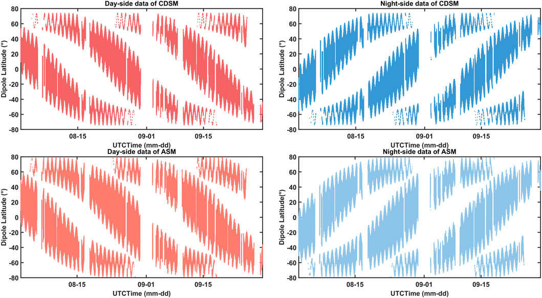
FIGURE 2. Data distribution of the CDSM and ASM for the period from 31 July 2019 to 30 September 2019 after the data screening.
In the figure, the selected data are distributed at most of the geomagnetic dipole latitude ranges. The datasets are abundant, and the statistical analysis can be statistically representative.
2.2 Cross Comparison
As was assumed before, the data of the two payloads are not exactly identical to each other in time and location. So, the CHAOS-7.8 model was used to calculate the magnetic field intensity of the corresponding model value using the same parameters such as UTC time, altitude, longitude, and latitude. A core field of spherical harmonic degree 20 and a crustal field of degree 110 were adopted.
For every data point, there are scalar magnetic field values measured by satellites in orbit and calculated by models in correspondence with each other. The difference between the measured value and the model value can indicate the deviation of the satellite in-orbit magnetic field measured data from the model. The calculation is applied in the equation:
where
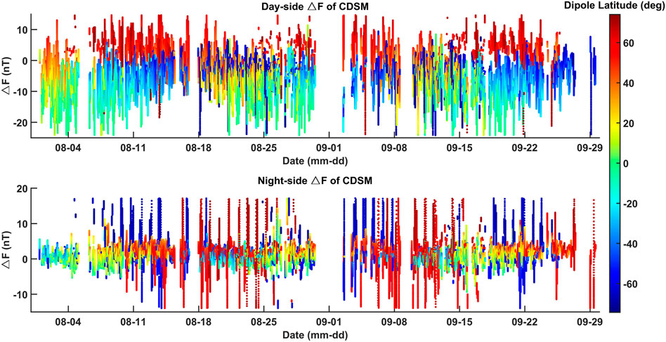
FIGURE 3.
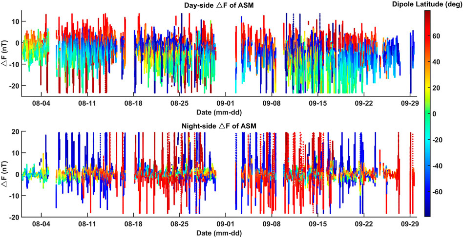
FIGURE 4.
As shown in the figures,
2.3 Methods of Analysis
By virtue of the CHAOS model, the indirect comparison analysis was realized. The
The mean value and standard deviation analysis can intuitively show the characteristics of
The mean values and standard deviations of the differences were calculated with a 10° resolution of the dipole latitude (Pollinger et al., 2020). On this basis, the differences of
3 Analysis Results and Discussion
According to the scheme and methods, some visualized results are obtained, which are displayed as follows, including the distribution of the difference between in-orbit data and the CHAOS model on the global scale and along dipole latitude and the mean value and standard deviation analysis.
3.1 Difference Between In-Orbit Data and Model Value
Focusing on the data selected which were distributed on some orbits from the dates of 31 July 2019 to 30 September 2019, the corresponding location in the geomagnetic coordinate of the Swarm Bravo data was calculated using IGRF-13 (Alken et al., 2021). Figure 5 shows the distribution of
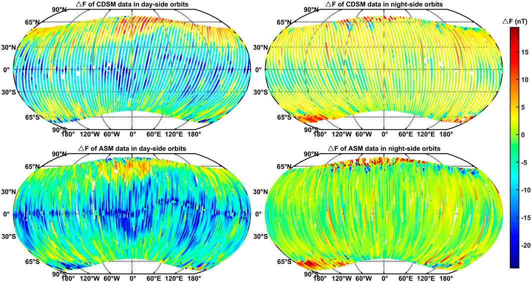
FIGURE 5. Distribution of
It can be seen from the figure that the
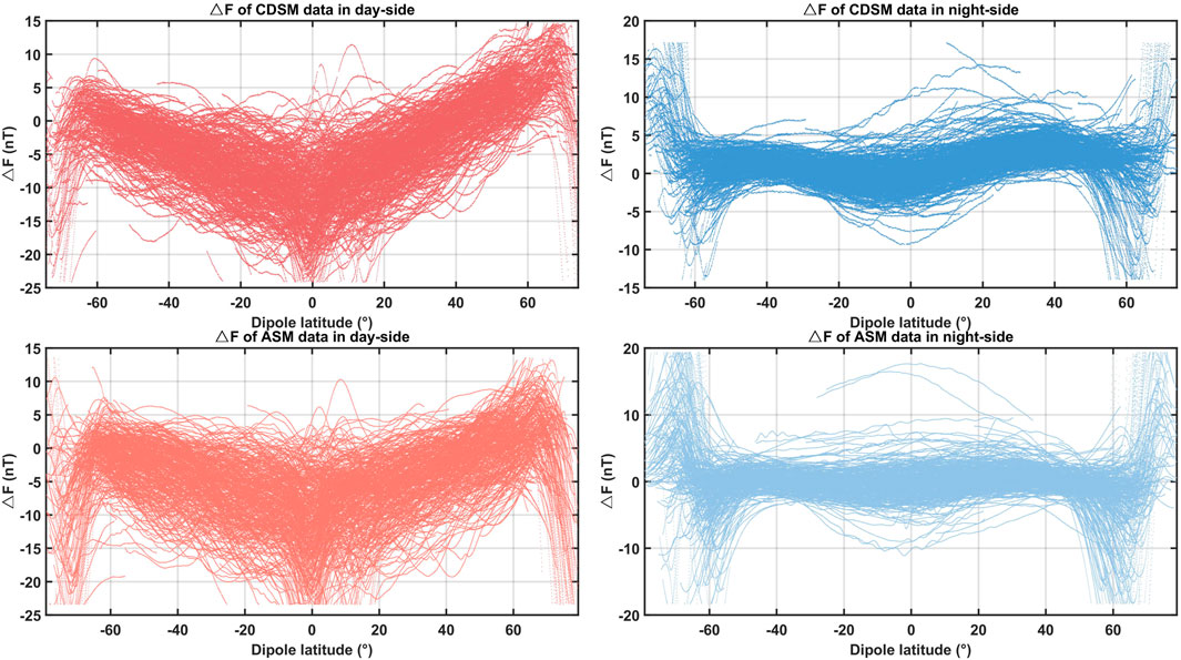
FIGURE 6.
Overall, the CDSM data and ASM data showed a good agreement in the figure. The data in the middle-latitude region are close to the model value,
3.2 The Mean Value and Standard Deviation Analysis
The scalar residuals between CHAOS and Swarm magnetic field data are much larger in the auroral region because of the presence of field-aligned currents. It is to be noted that the Swarm data have been used to generate the CHAOS model; therefore, it is expected that scalar residuals should be small but dependent on the current systems not included in the CHAOS model (Finlay et al., 2015). After considering the purpose of the study comprehensively, the suitable data from 31 July 2019 to 30 September 2019 of dipole latitude within the range of -60° to 60° were concentrated on. The mean value and standard deviation of
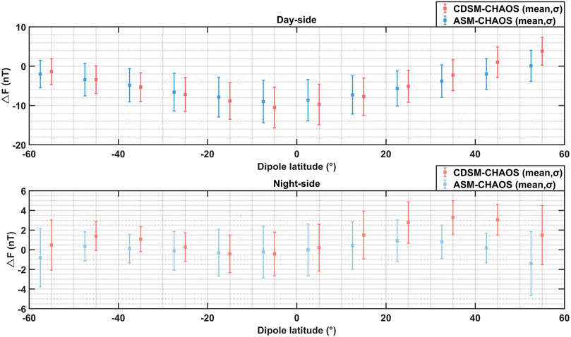
FIGURE 7. Error bars of
The mean values of
It can be seen that the error bars start to separate at dipole latitudes greater than 20° (Pollinger et al., 2020). These error bars of the CDSM are very similar to those of the ASM in other dipole latitude regions, so subtraction using both the mean value and standard deviation was performed in Figure 8. Also, it indicates that the data of both instruments are relatively consistent and stable.
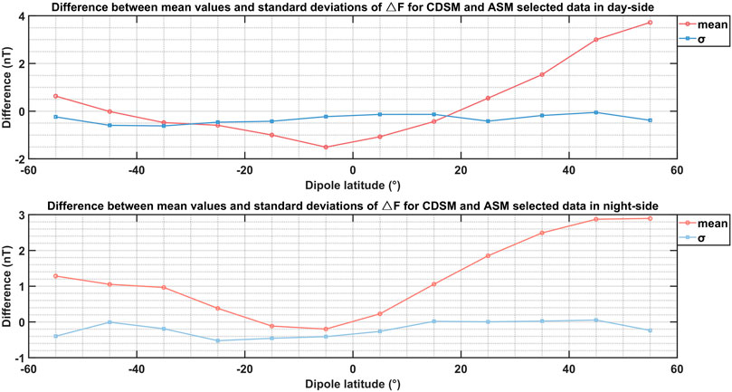
FIGURE 8. Difference between mean values and standard deviations of ∆F for the CDSM and for ASM selected data from July 31 to 30 September 2019.
It reflects that the deviation of the in-orbit scalar magnetic field measurement value is small compared with the value of the CHAOS model. The mean value and standard deviation distribution of the CDSM and ASM show a similar variation trend, and the dispersion is weak, reflecting a good consistency. Especially in middle- and low-latitude areas such as −30 to 10°, where the mean values fluctuate around 0, the standard deviation is smaller and the consistency is better.
3.3 Analysis Applying Other Scales
The equivalent analysis process was carried out with other spatial–temporal scales using the datasets from 31 July 2019 to 30 August 2019. The time interval between satellite data points was set to be 30 min, while the spatial distances were analyzed from 1° × 1° to 20° × 20°, considering non-overlapping range selections in order to understand the effect of data selected in specific ranges. Statistical analysis in terms of mean values and standard deviations was carried out. The results are shown in Figure 9.
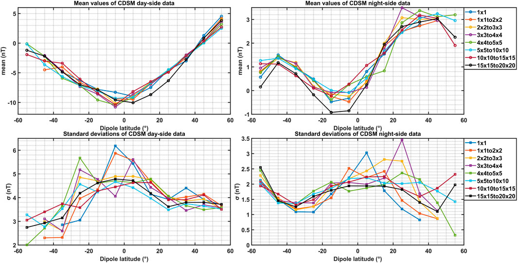
FIGURE 9. Statistical results of mean values and standard deviations of
These aforementioned curves have very similar variation trends and cross each other, and these mean values remain close to each other. On the night side, the difference of mean values between different curves is within 0.65 nT in the dipole latitude range of −40° to −30° and 30° to 40°, where the CHAOS model is thought to be the most accurate (Finlay et al., 2015). As the different datasets used for the figure are non-overlapping, the dataset amounts of different scales were examined and are shown in Table 1. It can be inferred that the influence on the results with different spatial scales is slight.

TABLE 1. Amounts of data on different spatial scales with the time interval being 30 min (For each category Day side/Night side, there are two lines: the first contains all data between 0 and the corresponding distance, the second only data between successive ranges.).
The selection of spatial distance being 10°×10° and time intervals being 60, 120, and 180 min with the Kp index lower than 2 + using data of September 2019 was carried out. Also, the non-overlapping time window is used and additional data are focused on. Figure 10 shows the statistical results of mean values and standard deviations of
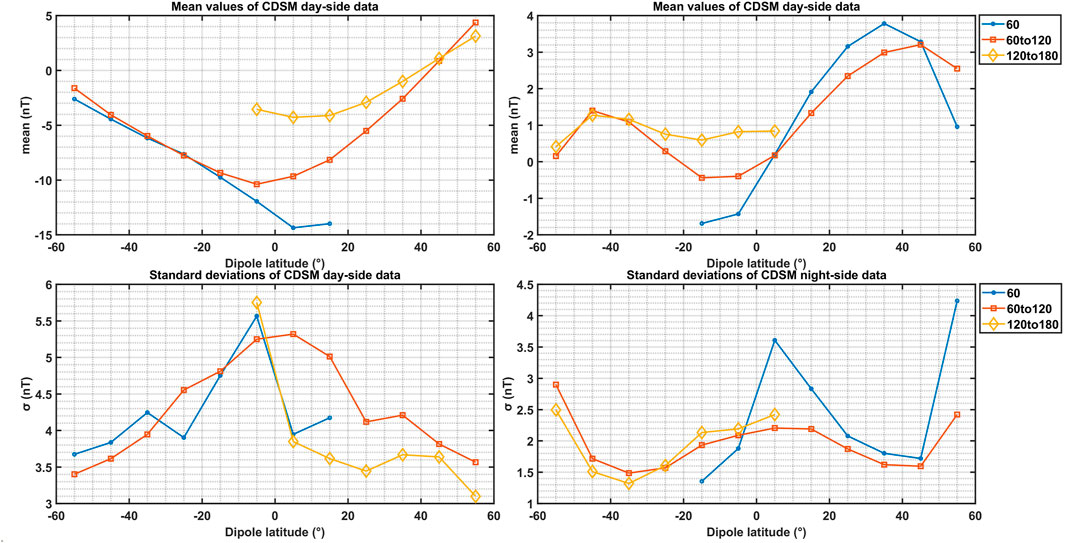
FIGURE 10. Statistical results of mean values and standard deviations of
As shown in the aforementioned figure, the statistical results of mean values and standard deviations of
Due to the orbital configuration of the satellites, sometimes the increase of a time window or spatial range did not allow to include additional data and cover all the latitude ranges, as can be seen in Figures 9, 10, where not all the various curves are completely distributed across all latitude ranges.
As the spatial–temporal scale was amplified, the suitable data volume generally had an increasing trend. But, the statistical analysis results seem similar with different non-overlapping datasets. It can be inferred that the selection of different spatial–temporal scale standards has no obvious influence on the statistical results, which means that the results are not sensitive to the change in time interval and spatial distance.
It is necessary to choose a scale with both time interval and spatial distance in order to select sufficient data to accomplish a comparison analysis of consistency. As for the research process, the data size and workload need to be considered. To ensure that the computation is convenient for the implementation of subsequent analysis, an appropriate time interval (180 min) and an appropriate spatial scale (5° × 5°) was adopted, and proper data size can be derived to reveal the actual situation of the in-orbit data. The restriction of the Kp index and data flag parameters should also be applied. It can be seen in these aforementioned curves that there are discrepancies in the results of different dipole latitude ranges and between the day-side and night-side, so the analysis and results discussion can focus on middle-latitude data on the night side, which are less disturbed and more credible. For long-term comparison, data from 2019 to 2020 were acquired, selected, and analyzed. It is to be noted that 2019 was during the solar minimum; therefore, the comparison results are credible.
3.4 Application to the Swarm Alpha satellite
In order to verify the applicability and effectiveness of the data screening methods and the approach of using models to compare data from different satellites, the same analysis process was also applied to the scalar magnetic field data of Swarm Alpha. Mean value and standard deviation analysis using scalar magnetic field data of CSES and Swarm Alpha from August to September 2019 was completed. Figure 11 shows the results of selected data using the criterion of time interval being 180 min and spatial distance being 5°×5°, distributed from August 25 to 29 September 2019. The dataset size used in the figure is 244337 and 242416 for the CDSM on the day side and night side and 308306 and 300724 for Swarm Alpha ASM on the day side and night side.
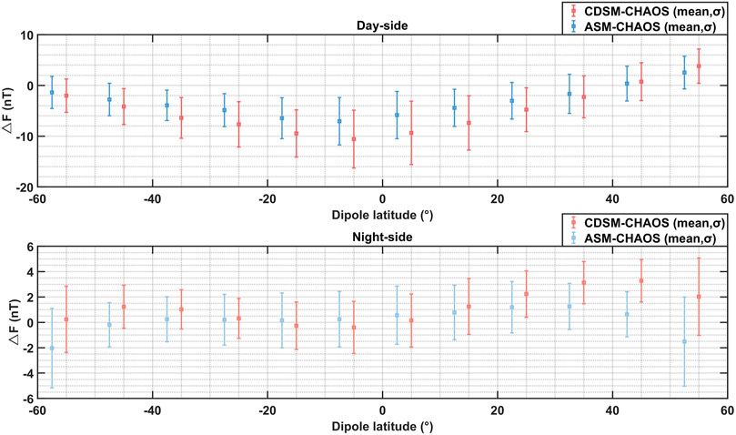
FIGURE 11. Error bars of
It can be seen that the mean values and standard deviations of the CDSM and Swarm Alpha ASM show similar variation trends, meaning that the data of CDSM onboard CSES and ASM onboard Swarm Alpha have good consistency with each other. The results show that the methods are also applicable and effective for similar data comparison studies between other satellites. In this study, the analysis of long-term data mainly focuses on CSES and Swarm Bravo satellites.
3.5 Analysis for the Long-Term In-Orbit Data
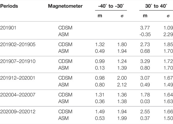
Adopting the time interval (180 min) and the spatial scale (5° × 5°), the long-term in-orbit data of CDSM and Swarm Bravo ASM from 2019 to 2020 were analyzed. After the data screening process, there were six periods with a significant amount of data satisfying the selection criteria, consisting of January 2019, February to May 2019, July to October 2019, December 2019 to January 2020, April to July 2020, and September to December 2020. The statistical results of these periods are shown as error bars in Figure 12.
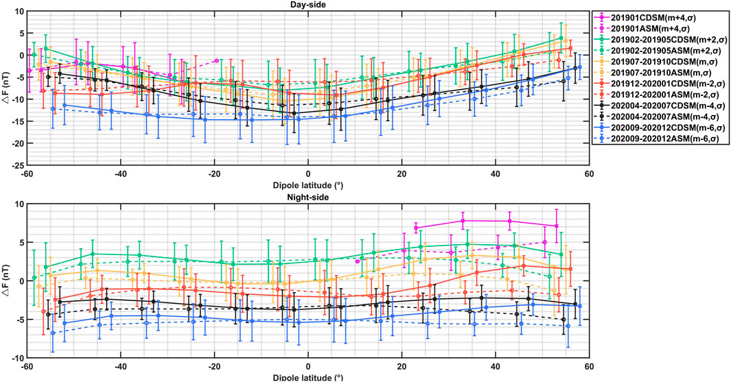
FIGURE 12. Mean value and standard deviation analysis of
The quantitative results of dipole latitude range of -40° to -30° and 30° to 40° on the night side are shown in Table 2.
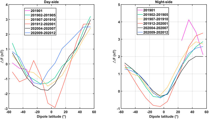
It is shown that in all these periods, the in-orbit data of both the CDSM and ASM agree with the CHAOS model value; thus, the inference can be drawn that they are relatively consistent with each other. Subtraction using the mean values of both the CDSM and ASM was carried out in Figure 13.
Analogously, the night-side data show great consistency with the model value. The CHAOS model is generated using the observation data from satellites including Swarm and optimized for the night side, which may explain the reason why the results for Swarm Bravo on the night side seem more accurate. Also, the distribution patterns have a similar trend with dipole latitude in different periods, indicating that both payloads are in stable operation and the quality of their data is stable overtime.
Using all the selected data of January 2019, February to May 2019, July to October 2019, December 2019 to January 2020, April to July 2020, and September to December 2020 after screening, statistical analysis was performed. As the CHAOS model is optimized for the night side and there may be solar illumination influencing the day-side data, only the night-side data were analyzed. Statistics were calculated in terms of date, and the mean value of every single day was calculated using
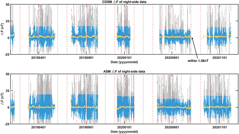
FIGURE 14. Statistical results of the difference between the CDSM/ASM and CHAOS using selected data from 2019 to 2020 (gray points represent the
As shown in these different colors, the 3 sigma criterion filtered the outliers effectively, which can reduce the influence of ionospheric perturbation and make the results more reliable. The daily mean values show a relatively stable trend in the long term for both the CDSM and ASM. The variation of most CDSM daily mean values during the period of April to July 2020 is within 1.58 nT. Some average daily
4 Conclusion
The CSES and Swarm satellites have similar altitudes and payloads, both operating well in orbit for a relatively long period. To carry out the cross comparison analysis, the condition was applied that their time interval and spatial distance are close enough to perform the consistency analysis. After setting the standards and data screening, the data which meet our requirements were acquired. As the data of the CDSM and ASM are not exactly identical in the parameters such as geographic longitude and latitude, altitude, and UTC time, the CHAOS-7.8 model was used to calculate the model value and realize the indirect comparison analysis. Then, the difference between the in-orbit data and model value was visualized in some statistical approaches.
In this study, the data screening methods are studied and described. The scales of spatial distance were used to limit the difference between the longitudes and latitudes of the CDSM and ASM, and the scales of the time interval are used to limit the difference between the UTC time of the CDSM and ASM. Several spatial–temporal scales were set up, with spatial distances ranging from 1° × 1° to 20° × 20° and time intervals varying from 30 min to 180 min. Data were selected for quiet periods with Kp lower than 2+ and the data flags were examined. The results of the comparison of different scales showed that the selection of spatial–temporal scales has no obvious influence on the final results. But the data size and workload need to be considered. To ensure that the computation is convenient for the implementation of subsequent analysis and the dataset size is statistically representative, an appropriate time interval (180 min) and an appropriate spatial scale (5° × 5°) can be adopted, and the statistical results can reflect the data quality in the long-term detection.
Applying this method, the short-term data comparison analysis for CDSM of CSES and ASM of both Swarm Alpha and Bravo in August and September, 2019, and the long-term data comparison analysis of the CDSM and Swarm Bravo ASM from 2019 to 2020 were realized. The conclusion in this study well supports the conclusion of (Pollinger et al., 2020). According to the results of the night-side orbit data, both scalar magnetic field data are in good agreement with the CHAOS model and are relatively consistent and stable. It can be inferred that the scalar magnetic field detection payloads of the two satellites have maintained long-term stability in orbit and obtained high-quality data.
Data Availability Statement
Publicly available datasets were analyzed in this study. The CSES datasets for this study are available at https://leos.ac.cn/#/home. The Swarm datasets for this study are available at https://earth.esa.int/eogateway/missions/swarm/data. The CHAOS-7 model is publicly available at https://www.spacecenter.dk/files/magnetic-models/CHAOS-7/index.html. The Kp index data can be obtained at http://wdc.kugi.kyoto-u.ac.jp/wdc/Sec3.html.
Author Contributions
JZ and BC carried out the data analysis. YT, YM, and BZ contributed to the development of the methodology. AP, XZ, and YY contributed to the analysis of CDSM data. XG, YZ, JW, and LL contributed to the discussion of the results. WM, RL, ZZ, and XS provided comments on the discussion of the results. All authors read and approved the final manuscript.
Funding
This article is supported by the National Key Research and Development Program of China from the Ministry of Science and Technology of the People´s Republic of China (MOST) (grant no. 2018YFC1503501) and the NSFC (grant no. 41904147). Work of PA, MW, and LR was supported by the Austrian Space Applications Programme (Grant No. 873688).
Conflict of Interest
Authors MY and ZX are employed by DFH Satellite Co. Ltd.
The remaining authors declare that the research was conducted in the absence of any commercial or financial relationships that could be construed as a potential conflict of interest.
Publisher’s Note
All claims expressed in this article are solely those of the authors and do not necessarily represent those of their affiliated organizations, or those of the publisher, the editors, and the reviewers. Any product that may be evaluated in this article, or claim that may be made by its manufacturer, is not guaranteed or endorsed by the publisher.
Acknowledgments
This work made use of the data from the CSES mission, a project funded by the China National Space Administration (CNSA) and the National Institute of Natural Hazards, Ministry of Emergency Management of China (NINH). The authors gratefully acknowledge support from CSES teams for providing CDSM data and ESA Swarm teams for providing ASM data for long-term analysis.
References
Alken, P., Thébault, E., Beggan, C. D., Amit, H., Aubert, J., Baerenzung, J., et al. (2021). International Geomagnetic Reference Field: the Thirteenth Generation. Earth, Planets Space 73 (1). doi:10.1186/s40623-020-01288-x10.1186/s40623-020-01281-4
Cheng, B., Zhou, B., Magnes, W., Lammegger, R., Pollinger, A., Ellmeier, M., et al. (2015). “Performance of the Engineering Model of the CSES High Precision Magnetometer,” in 2015 IEEE SENSORS, 1–4. doi:10.1109/icsens.2015.7370679
Cheng, B., Zhou, B., Magnes, W., Lammegger, R., and Pollinger, A. (2018). High Precision Magnetometer for Geomagnetic Exploration Onboard of the China Seismo-Electromagnetic Satellite. Sci. China Technol. Sci. 61 (5), 659–668. doi:10.1007/s11431-018-9247-6
Finlay, C. C., Kloss, C., Olsen, N., Hammer, M. D., Tøffner-Clausen, L., Grayver, A., et al. (2020). The CHAOS-7 Geomagnetic Field Model and Observed Changes in the South Atlantic Anomaly. Earth Planets Space 72 (1), 156. doi:10.1186/s40623-020-01252-9
Finlay, C. C., Olsen, N., and Tøffner-Clausen, L. (2015). DTU Candidate Field Models for IGRF-12 and the CHAOS-5 Geomagnetic Field Model. Earth Planet Sp. 67 (1). doi:10.1186/s40623-015-0274-3
Fratter, I., Léger, J.-M., Bertrand, F., Jager, T., Hulot, G., Brocco, L., et al. (2016). Swarm Absolute Scalar Magnetometers First In-Orbit Results. Acta Astronaut. 121, 76–87. doi:10.1016/j.actaastro.2015.12.025
Matzka, J., Bronkalla, O., Tornow, K., Elger, K., and Stolle, C. (2021). Geomagnetic Kp Index. V. 1.0. Potsdam, Germany: GFZ Data Services. doi:10.5880/Kp.0001
National Institute of Natural Hazards Ministry of Emergency Management of China (2020). China Seismo-Electromagnetic Satellite (ZH-1(01)) the L2/2A Data Product Description[S].
National Space Institute Technical University of Denmark (2019). Swarm Level 1b Product Definition[S]. Kongens Lyngby, Denmark: SW-RS-DSC-SY-0007. Issue 5.23.
Olsen, N., and Floberghagen, R. (2018). Exploring Geospace from Space: the Swarm Satellite Constellation Mission. Space Res. Today 203, 61–71. doi:10.1016/j.srt.2018.11.017
Olsen, N., Lühr, H., Sabaka, T. J., Mandea, M., Rother, M., Tøffner-Clausen, L., et al. (2006). CHAOS-a Model of the Earth's Magnetic Field Derived from CHAMP, Ørsted, and SAC-C Magnetic Satellite Data. Geophys. J. Int. 166 (1), 67–75. doi:10.1111/j.1365-246X.2006.02959.x
Pollinger, A., Amtmann, C., Betzler, A., Cheng, B., Ellmeier, M., Hagen, C., et al. (2020). In-orbit Results of the Coupled Dark State Magnetometer Aboard the China Seismo-Electromagnetic Satellite. Geosci. Instrum. Method. Data Syst. 9 (2), 275–291. doi:10.5194/gi-9-275-2020
Shen, X., Zhang, X., Yuan, S., Wang, L., Cao, J., Huang, J., et al. (2018). The State-Of-The-Art of the China Seismo-Electromagnetic Satellite Mission. Sci. China Technol. Sci. 61 (5), 634–642. doi:10.1007/s11431-018-9242-0
Yang, Y., Hulot, G., Vigneron, P., Shen, X., Zhima, Z., Zhou, B., et al. (2021). The CSES Global Geomagnetic Field Model (CGGM): an IGRF-type Global Geomagnetic Field Model Based on Data from the China Seismo-Electromagnetic Satellite. Earth Planets Space 73 (1). doi:10.1186/s40623-020-01316-w
Keywords: China Seismo-Electromagnetic Satellite, Swarm Satellites, magnetometer, scalar magnetic field, cross comparison analysis
Citation: Jianing Z, Bingjun C, Yuqi T, Yuanqing M, Bin Z, Andreas P, Xinghong Z, Yanyan Y, Xiaochen G, Yiteng Z, Jindong W, Lei L, Werner M, Roland L, Zhima Z and Xuhui S (2022) Comparison of Scalar Magnetic Field Data of China Seismo-Electromagnetic Satellite and Swarm Bravo Satellite. Front. Earth Sci. 10:866438. doi: 10.3389/feart.2022.866438
Received: 31 January 2022; Accepted: 23 23 May 20222022;
Published: 12 July 2022.
Edited by:
Mirko Piersanti, University of L'Aquila, ItalyReviewed by:
Pierdavide Coïsson, UMR7154 Institut de Physique du Globe de Paris (IPGP), FranceFan Yin, Wuhan University, China
Copyright © 2022 Jianing, Bingjun, Yuqi, Yuanqing, Bin, Andreas, Xinghong, Yanyan, Xiaochen, Yiteng, Jindong, Lei, Werner, Roland, Zhima and Xuhui. This is an open-access article distributed under the terms of the Creative Commons Attribution License (CC BY). The use, distribution or reproduction in other forums is permitted, provided the original author(s) and the copyright owner(s) are credited and that the original publication in this journal is cited, in accordance with accepted academic practice. No use, distribution or reproduction is permitted which does not comply with these terms.
*Correspondence: Cheng Bingjun, Y2hlbmdiakBuc3NjLmFjLmNu
 Zhang Jianing
 Cheng Bingjun
 Tong Yuqi1,2
 Zhou Bin
 Zhang Yiteng
 Magnes Werner