Application of GPR System With Convolutional Neural Network Algorithm Based on Attention Mechanism to Oil Pipeline Leakage Detection

High-efficiency and high-quality detection of oil pipeline will significantly reduce environmental pollution and economic loss, so an unconventional oil pipeline anomaly detection convolutional neural network (CNN) algorithm based on attention mechanism is proposed in this article. By taking the simulated ground-penetrating radar (GPR) data as prior knowledge, the structure of the convolutional neural network based on the attention mechanism is constructed, and finally, the location and working condition of the underground oil pipeline are recognized in the simulation data and measured data. The simulation results show that after using the new optimized convolutional neural network, the accuracy rates of the leakage discrimination from horizontal data acquired along the oil pipeline and the classification of the target from longitudinal data acquired perpendicular to the oil pipeline are 94.5% and 84.6%, respectively. Compared with the original convolutional neural network without an attention mechanism, the accuracy rates of the leakage discrimination and the classification of the target are improved by 6.2% and 7.8%, respectively. We further train measured data with an optimized convolutional neural network, results show that compared with a conventional network, the new network can increase the corresponding accuracy rates of the leakage discrimination and the targets classification by 5.4% and 6.9%, reaching 92.3% and 84.4%, respectively. According to our study, the ground-penetrating radar oil pipeline recognition algorithm based on an attention mechanism can well accomplish the identification of underground oil pipelines.

Introduction

The rapid development of the petroleum industry makes the research on the safety of oil storage and transportation meaningful (Hu et al., 2021). The oil pipeline has become an important choice for oil transportation because of its high safety, high speed, and reasonable cost (Chen et al., 2018). Under the influence of external factors, the oil pipeline running for a long time is prone to leakage problems. After the oil pipeline leaks, it will not only waste a lot of resources and cause economic loss, but also seriously pollute the environment and affect human life. Efficient and high-quality detection of oil pipelines will be able to monitor leakage in time and effectively reduce resource waste and environmental pollution (Wang et al., 2014). Therefore, an unconventional oil pipeline anomaly detection algorithm based on the attention mechanism is proposed.

Up to now, there are many detection methods for oil pipeline leakage. For example, the negative pressure wave method, ultrasonic detection method, optical fiber detection method, etc. Negative pressure wave method is safe and simple. It also has a wide detection range and fast response. However, this method is difficult to successfully detect small and slow leakage (Liang et al., 2010). The ultrasonic detection method is complex and needs to fill the coupling agent between the probe and the pipe wall (Yang et al., 2021). The optical fiber detection method has good security and high sensitivity, but it needs to add appropriate isolation materials and has a high cost (Zhou et al., 2019; Zhao et al., 2021). Instead, the ground-penetrating radar(GPR) has the characteristics of being nondestructive, high efficiency, having high imaging resolution, and penetrability (Cao et al., 1996). It is widely used in road and bridge detection, building quality analysis as well as underground target detection and classification (Hinton and Salakhutdinov, 2006; Vargas et al., 2017). After comprehensive consideration, the unconventional method of ground-penetrating radar is proposed to detect the state of the underground oil pipeline.

Interpretation of ground-penetrating radar (GPR) section data highly depends on the subjective judgment of experts, which takes a long time and has the risk of misjudgment (Kunihiko and Sei, 1982; Lu and Zhang, 2016; Wanjun et al., 2016). Therefore, it is of great significance to explore an efficient automatic underground target recognition algorithm. Several research studies have been carried out to realize the automatic recognition of GPR section features (Jia et al., 2007; Liu et al., 2017). The most classic image recognition algorithm in GPR is Hough transform, mainly used to identify hyperbola in GPR images (Windsor et al., 2013; Li et al., 2016). However, due to the diversity of detected targets, the corresponding signals of targets in GPR images are not limited to hyperbola but complex and diverse. Dictionary learning method and template matching method are also commonly used GPR image recognition algorithms (Sagnard and Tarel, 2016; Terrasse et al., 2016). But those similar approaches rely heavily on dictionary models and templates, requiring a lot of parameter configurations.

With the gradual maturity of deep learning, it has been widely used in exploration techniques in recent years, such as fracturing design optimization, sweet spot detection, production forecasting, GPR data interpretation, etc, (Wang and Chen, 2019; Tang et al., 2020; Xiong et al., 2020). Lei W et al. (2019) used the R-CNN network to identify hyperbolic features in GPR B-scan images. It can determine whether there are buried objects in the detected underground space. Kang et al. (2020) constructed 3D radar data of underground targets, and then put it in the deep convolutional neural network for training. The accuracy of cavity and pipeline classification was 92% and 98%, and the false alarm rate was 8% and 2%, respectively. Lei et al. (2020) combined the convolutional neural network and the long-short-term memory artificial neural network to extract the hyperbola in the B-scan image of the ground-penetrating radar. However, the existing research mainly focuses on the data processing of the whole B-scan image. Classification output often stays in the recognition of the whole image, and its main research objectives are the existence of underground targets and the recognition of target materials. Further exploration of the geometric features, size, condition, and position of the target is still insufficient. Therefore, a novel convolutional neural network based on the attention mechanism is proposed for further feature recognition of the underground oil pipelines.

Numerical Simulation Mechanism and Realization of Underground Oil Pipeline

A GPR oil pipeline recognition system based on the attention mechanism requires a lot of training and test data, which need to be real data or close to them. The data obtained by electromagnetic simulation can be generated in batches with simple locations. Moreover, the target location is clear from the data, and the actual situation can be accurately represented. Therefore, a large amount of electromagnetic simulation data is initially obtained in this study to provide data support for neural network construction. Furthermore, these simulation data help a lot for the acquisition, processing, and network structure adjustment of measured data.

To achieve a reasonable numerical simulation of underground pipeline objects in an interested environment, a direct relationship between soil physical properties and the overall dielectric response of soil components (soil particles, water, and air) is established using dielectric mixing models. According to a semi-empirical model proposed by Peplinski et al. (1995), the soil simulation model is constructed to simulate the electromagnetic properties of real soil. In this model, the soil is composed of clay, silt, and sand. The diameter of clay, silt and sand is below 0.002, 0.002–0.02 mm, and 0.02–2 mm, respectively. Different soil types can be constructed by changing the proportions of different components. Soil water content also has a certain influence on its electromagnetic properties. Therefore, the complex permittivity of soil $\epsilon \left(\omega \right)$ can be expressed as Eq. 1:

$\epsilon \left(\omega \right)={\epsilon }^{\prime }\left(\omega \right)-j{\epsilon }^{″}\left(\omega \right)(1)$

${\epsilon }^{\prime }\left(\omega \right)=1.15{\left[1+\frac{{\rho }_b}{{\rho }_s}\left({\epsilon }_s^{\alpha }\right)+m_v^{{\beta }^{\prime }}{{\epsilon }^{\prime }}_{fw}^{\alpha }-m_v\right]}^{1/\alpha }-0.68(2)$

${\epsilon }^{″}\left(\omega \right)=\left[m_v^{{\beta }^{″}}{{\epsilon }^{″}}_{fw}^{\alpha }\right](3)$

In the aforementioned formula, ${\epsilon }^{\prime }\left(\omega \right)$ and ${\epsilon }^{″}\left(\omega \right)$ are the real and imaginary parts of the complex dielectric constant $\epsilon \left(\omega \right)$, respectively. ${\rho }_b$ and ${\rho }_s$ are the total density of soil and the density of sandy soil composition (unit: g/cm3), respectively. $a$ is an empirical constant with a value of 0.65. ${\beta }^{\prime }$ and ${\beta }^{″}$ are the constants related to soil composition, and their expressions are:

${\beta }^{\prime }=1.2748-0.519S-0.152C(4)$

${\beta }^{″}=1.33797-0.603S-0.166C(5)$

where $S$ and $C$ are the proportions of sand and clay, respectively (0 < $S$ < 1, 0 < $C$ < 1).

In Eqs 2, 3, ${{\epsilon }^{\prime }}_{fw}$ and ${{\epsilon }^{″}}_{fw}$, respectively, represent the real and imaginary parts of free water in the soil, and their expressions are:

${{\epsilon }^{\prime }}_{fw}={\epsilon }_{w\infty }+\frac{{\epsilon }_{w0}-{\epsilon }_{w\infty }}{1+{\left(2\pi f{\tau }_w\right)}^2}(6)$

${{\epsilon }^{″}}_{fw}=\frac{2\pi f{\tau }_w\left({\epsilon }_{w0}-{\epsilon }_{w\infty }\right)}{1+{\left(2\pi f{\tau }_w\right)}^2}+\frac{{\sigma }_{eff}}{2\pi {\epsilon }_{0}f}\frac{\left({\rho }_s-{\rho }_b\right)}{{\rho }_s{m}_v}(7)$

${\epsilon }_{w\infty }$ is the limit of ${{\epsilon }^{″}}_{fw}$ at high frequencies. ${\tau }_w$ is the relaxation time constant of free water. ${\epsilon }_{w0}$ is the static relative permittivity of water, and its value is 80.1. ${\sigma }_{eff}$ is the effective conductivity, which is given by the empirical Eq. 8:

${\sigma }_{eff}=0.0467+0.2204{\rho }_b-0.4111S+0.6614C(8)$

Through the aforementioned mechanism, the real soil environment can be simulated and fitted. Figure 1 shows the experimental configuration when using GPR to obtain B-scan data of the oil pipeline. We set the length of the entire space as L, ranging from 500 to 2500 cm, the height to 200 cm, the width to 100 cm, and the diameter of the single grid to 2 cm. Soil consists of variable sand and clay with a density of 2.66 and 2 g/cm³, respectively. Its water content varied from 0.1% to 1%. The frequency of the antenna is selected from 100 to 600 Mhz. The initial position of the antenna is 20 cm from the left edge of the model, and the distance between transmit and receive antennas is 5 cm. The acquisition of the horizontal B-scan data along the oil pipeline is shown in Figure 1A. The radius of the oil pipeline is set as R, ranging from 10 to 72 cm. The depth of the oil pipeline is H1 with the range of 0 to (200-2R) cm. When the oil pipeline leaks, the depth of leakage area is depicted as H2, changing from 0 to 200 cm according to the position of the oil pipeline. Similarly, the acquisition of longitudinal B-scan data perpendicular to the oil pipeline is shown in Figure 1B. The radius of oil pipeline 1 is R1, varying from 10 to 72 cm. The depth of 1 is H1 with the range of 0 to (200-2R) cm. When leakage occurs, the depth of leakage area is H2, ranging from 0 to 200 cm according to the position of the oil pipeline. The depth of oil pipeline 2 is H3 and the radius is R2, which is consistent with those of oil pipeline 1.

FIGURE 1

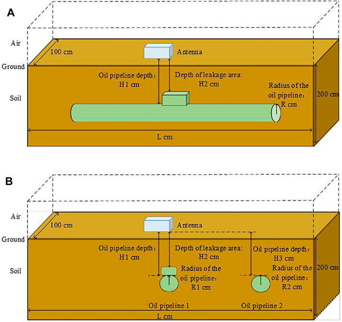
FIGURE 1. Experiment configuration when obtaining oil pipeline B-scan data by GPR. (A) Acquisition model of horizontal B-scan data along oil pipeline; (B) acquisition model of longitudinal B-scan data perpendicular to the oil pipeline.

The simulated B-scan data of the oil pipeline are obtained using the experimental setup for the field measurement with GPR. Figures 2A and B show the three-dimensional (3D) simulation model of the oil pipeline under the condition of normal operation and leakage, respectively. The pipeline is full of oil with a buried depth of 0.65m, a horizontal coordinate of 2.75 m, and a radius of 0.3 m. The leak area is filled with oil, directly below the oil pipeline. And its length, height, and width are set to 50, 30, and 50 cm, respectively. The soil is composed of 50% sand and 50% clay.

FIGURE 2

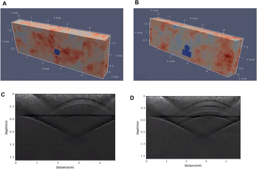
FIGURE 2. 3D and B-scan images of oil pipeline simulation model. (A) 3D image of normal operation; (B) 3D image of leakage; (C) B-scan image under normal operation; (D) B-scan under leaking condition.

Figures 2C and D show the corresponding simulation results of the two models in Figures 2A andB. A great difference exists in the B-scan image when leakage occurs or not. Concretely, the hyperbolas of the pipeline without leakage are more clear and non-intersecting, as shown in Figure 2C. Because the leakage area overlaps with the pipeline, a portion of the hyperbola representing leakage will intersect the original hyperbola of the pipeline, as shown in Figure 2D. Therefore, the GPR can clearly identify underground targets. However, due to the continuous reflection of electromagnetic waves among the leakage area, the pipeline area, and the stratum surface, the pipeline and leakage can only be clearly characterized at the top of the B-scan image. The hyperbolas superimpose on each other in Figure 2D and become too disordered to extract their representations.

Because no appropriate leaking oil pipelines exist, water is selected to replace oil to simulate leakage due to environmental pollution and safety issues. Figures 3A and B show 3D simulation model under the condition of normal operation and water leakage, respectively. The water pipeline has a buried depth of 0.4 m, a horizontal coordinate of 2.5 m, and a radius of 0.1 m. The leakage is a mixture of water and soil, with an area of about 0.06 m². The leftmost and rightmost horizontal coordinates of the leakage are 2.1 and 2.7 m, respectively. Both models use the stratified soil with a surface part composed of a mixture of sand and silt (70%) as well as clay (30%), and a bottom half composed of a mixture of sand and silt along with clay each accounting for 50%.

FIGURE 3

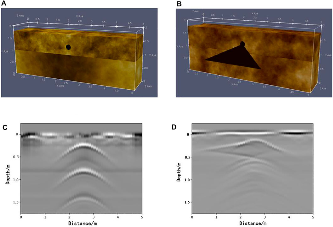
FIGURE 3. 3D and B-scan images of water pipeline simulation model. (A) 3D image of normal operation; (B) 3D image of leakage; (C) B-scan image under normal operation; (D) B-scan under leaking condition.

Figures 3C and D show the corresponding simulation results of the two models in Figures 3A and B. Similar to the B-scan images of oil pipelines, a great difference exists between water pipelines with and without leakage. The multiple disjoint and vertically distributed hyperbolas in Figure 3C are caused by the back and forth bounces of electromagnetic waves between the pipeline and the stratum surface. A horizontal line will also be generated at the formation interface due to the reciprocating reflections of electromagnetic waves between the formation interface and the surface. While in Figure 3D, the hyperbolas superimposed on each other and the characteristic echo at the formation interface is also not obvious.

In the batch generation of simulation data, parameters of each simulation model, such as soil composition, the shape, size, and working state of the target, and the obtained simulation results should be different. The simulation data generator replaces the random key parameters that need to be adjusted with placeholders and sets the predetermined range of the parameters. The process for producing bulk simulation data are demonstrated in Figure 4. Each time the program runs, the first step is to generate a model configuration file. During this procedure, parameters represented by placeholders will first generate and input data of a limited range into the configuration file. After saving the file, the program will realize the corresponding simulation operation.

FIGURE 4

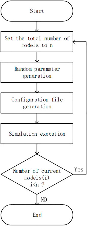
FIGURE 4. Flow chart of the program generating bulk simulation data.

Detection Model of Underground Oil Pipeline Based on Attention Mechanism

The attention model is divided into soft attention and hard attention. When choosing information, soft attention does not extract just one information from multiple information, but calculates the weighted average of this information and then inputs it into the neural network for calculation. Hard attention is to select a certain piece of multiple information, which can be selected according to the magnitude of the probability. Generally, the soft attention model is used to deal with neural network problems of its differentiable nature. There are three types of attention domain models in soft attention, namely the spatial domain model, the channel domain model, and the mixed domain model of them (Convolutional Block Attention Module, CBAM), which can extract attention in the channel and spatial dimensions (Woo et al., 2018). Compared with the attention mechanism that only focuses on one separate domain, it can achieve better results.

When the input feature is $F\in R^{L\times W\times C}$, and the three-dimensional information of the input feature map is L, W, and C. The final output feature map $F^{″}$ is obtained after the input feature map $F$ passes through the spatial attention module $M_S\in R^{L\times W\times 1}$ and the channel attention module $M_c\in R^{1\times 1\times C}$.

$F^{\prime }=M_c\left(F\right)\otimes F(9)$

$F^{″}=M_s\left(F\right)\otimes F^{\prime }(10)$

Because the input features and refined features are of a consistent size, the original parameters of the neural network remain unchanged after extraction by the CBAM module. The new features extracted by the convolutional neural network contain multiple channels representing different kinds of original ones, which have different effects on the final content identified by a convolutional neural network. While channel domain attention model is to generate the weight of each channel according to its degree of importance, and finally emphasizes attention to key channels as well as reduces attention to non-key ones. The structure of the channel domain attention model is shown in Figure 5A.

FIGURE 5

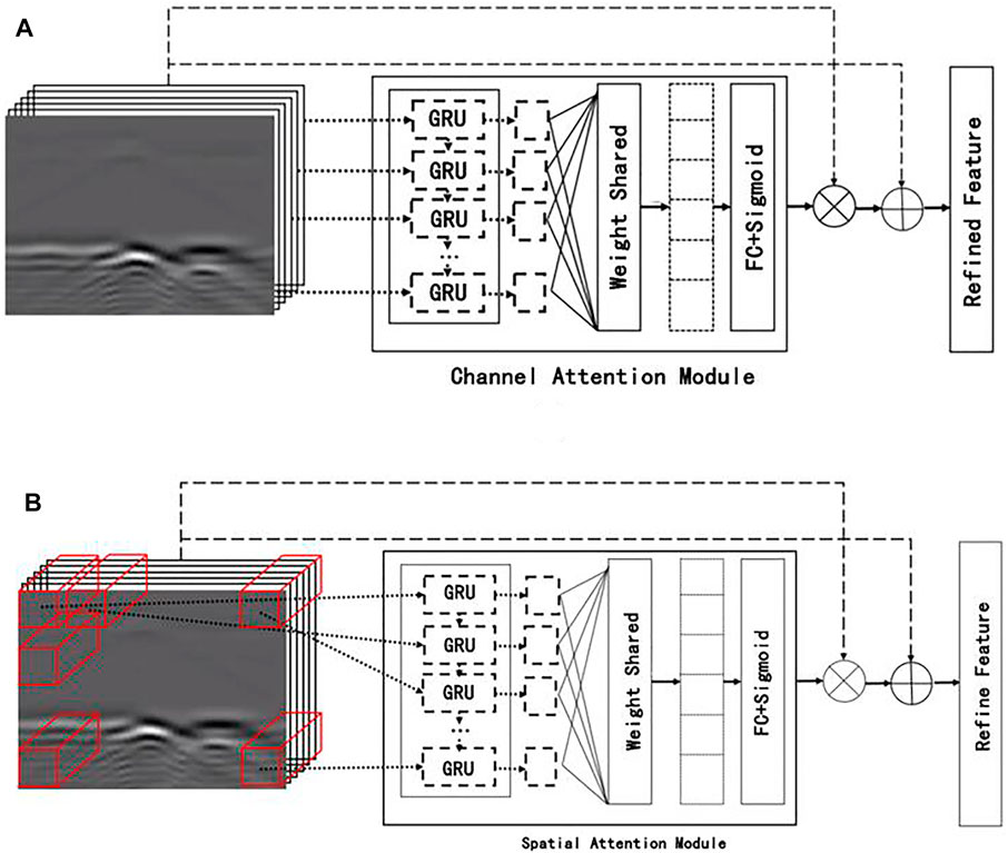
FIGURE 5. Structure diagram of attentional mechanism model. (A) Structure of channel domain attention model; (B) structure of spatial attention model.

The channel attention module initially uses the average and maximum pooling operations to aggregate the information of the feature map on each channel, and generates two different channel context descriptors $F_{mea}^c$ and $F_{\max }^c$, as shown in Eqs 11, 12:

$F_{mea}^c=\frac{1}{\mathit{L}\times \mathit{W}}{\displaystyle \sum _{i=1}^L{\displaystyle \sum _{j=1}^W{x}_c\left(i,j\right)}}(11)$

$F_{\max }^c=Max\left(x_c\left(i,j\right)\right),i\in \left[1,\mathit{L}\right],j\in \left[1,W\right](12)$

where $F_{\max }^c$ and $F_{mea}^c$ are the maximum and average pooling features on channel C, respectively. The length and width of the feature map are L and W, respectively. $x_c$ represents channel C.

Then average and maximum pooling features are input into the multilayer perceptron network, respectively. Combining the output values of them, the weight parameters of combined output feature can be obtained. The calculation formula is as follows:

$\begin{array}{c}{M}_c\left(F\right)=\sigma (mlp(P_{\mathit{mea}}\left(F\right))+mlp(P_{\mathit{max}}\left(F\right)))\\ =\sigma \left(w_1\left(w_0\left(F_{\mathit{mea}}^c\right)\right)+w_1\left(w_0\left(F_{\max }^c\right)\right)\right)\end{array}(13)$

where $P_{\mathit{max}}\left(F\right)$ and $P_{\mathit{mea}}\left(F\right)$ represent maximum and average pooling operations, respectively. $w_0$ and $w_1$ are the weight values of multi-layer perceptron. $\sigma$ represents the activation function.

There are various interferences when using GPR B-scan imaging, and the image content is complicated. It is particularly important to focus on and classify the regions with prominent features. Based on the features extracted by the convolutional neural network, the spatial domain attention model further explores the connections between features of different regions. In this way, weights of different regions are generated to highlight critical regions and weaken unimportant ones. The spatial attention module, delineated in Figure 5B, mainly focuses on the spatial relations among features and plays as a supplement to channel attention.

After average and maximum pooling of input features, two independent feature maps, $F_{mea}^s\in R^{L\times W\times 1}$ and $F_{\max }^s\in R^{L\times W\times 1}$, are generated.

$F_{\mathit{mea}}^s=\frac{1}{N}{\displaystyle \sum _{c=1}^N{s}_{ij}\left(c\right)}(14)$

$F_{\max }^s=Max\left(s_{ij}\left(c\right)\right),c\in \left[1,N\right](15)$

where N represents the number of feature channels, $s_{ij}\left(c\right)$ is the element at coordinates (i, j) on the cth feature map. $F_{\max }^s$ and $F_{\mathit{mea}}^s$ are the maximum and average fusion feature on each channel, respectively. After putting the two merged feature maps into the convolutional layer, we can get the attention weight in spatial dimension. Where $\sigma$ is the activation function, $f$ is the convolution operation, and n×n is the size of convolution kernel.

$\begin{array}{c}Ms\left(F\right)=\sigma \left(f^{n\times n}\left(\left[P_{\text{mea}}\left(F\right);P_{\text{max}}\left(F\right)\right]\right)\right)\\ =\sigma \left(f^{n\times n}\left(\left[F_s^{mea};F_s^{\max }\right]\right)\right)\end{array}(16)$

In order to identify the location and working state of an underground oil pipeline, the initial convolutional neural network structure is composed of a convolution layer, pooling layer, and full connection layer. The generalization ability of the network is weak, and the calculated accuracy rates of the horizontal pipeline leakage identification and longitudinal target location are low. In order to solve the problem of weak generalization ability and improve the accuracy rates, dropout technology is introduced. Dropout technology can mitigate overfitting and regularize. The core idea of dropout is to discard some neurons with a certain probability during network training. Then the over-fitting of the network is reduced and the generalization ability of the model is enhanced. In order to further improve the accuracy rates of the horizontal pipeline leakage identification and longitudinal target location, a convolutional attention module CBAM is introduced. The convolutional pooling operation in a convolutional neural network defaults to the same importance of each channel in the feature map. However, the amount of information carried by each channel is different, so it is unreasonable to assign the same importance to each channel. The convolutional attention module CBAM, based on the mechanism of the human visual system, will place more attention on important areas and reduce the weight of unimportant factors. Therefore, different feature maps and different regions of feature maps have different degrees of attention. Finally, the accuracy rates of the horizontal pipeline leakage identification and longitudinal target location are further improved.

Finally, in order to better recognize the horizontal position, state, depth, and cross-sectional area of the underground target, two convolutional neural networks based on the attention mechanism are proposed. They are the classification network for target horizontal position and state recognition, and the regression network for target depth and cross-sectional area detection.

Classification Network

The initial classification network and its relevant parameters are shown in Figure 6A and Table 1, respectively. However, the CBAM layer and dropout operation are not used. The network contains 4 convolutional layers, and the size of the convolution kernel in the first layer is set to 6 × 6 to modularize corresponding data features with high efficiency. The size of the following convolution kernel decreases with the progressively smaller feature map, which can increase the fitting expression ability of the network. Through these four convolution layers, the network can reduce the parameters and the amount of calculation while retaining the characteristics, and greatly improving the calculation efficiency. After each convolutional network layer, an attention module CBAM layer is added, which does not change the size and quantity of data but increases the weight of the key areas of the image. Add a pooling layer after the CBAM layer is to reduce data size and increase channel number. Then, two full connection layers and one output layer are designed. These three layers help classify the data extracted by the convolutional neural network. The last output layer is proposed to determine whether the output result is no target, pipeline, or pipeline leakage in the case of pipeline leakage detection. The activation function of this layer is softmax, which is suitable for data classification and can enable the network to represent the probability of each attributed type through machine learning. The maximum probability is set as the output target classification to further accomplish the classification and discrimination of the B-scan images.

FIGURE 6

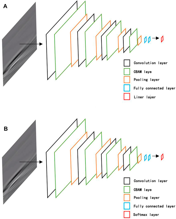
FIGURE 6. Block diagram of complete neural network. (A) Classification network model structure; (B) regression network model structure.

TABLE 1

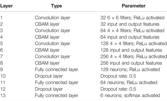
TABLE 1. Parameters of underground target recognition classification network structure.

Regression Network

The initial classification network its relevant parameters are shown in Figure 6B, but the CBAM layer and dropout operation are not used. For the prediction of target depth, the output function needs to be adjusted to give the discrete output value. Transformation is made on the basis of a classification network to construct the regression network. The target cross-sectional area and depth prediction can be carried out by changing the output layer function from softmax to liner, the output results of which are continuous real numbers. The front part of the regression network structure is the same as that of the classification network, and relevant parameters are adjusted during training to improve the recognition accuracy.

Simulation Results and Analysis

The convolutional neural network based on the attention mechanism is used to train the simulation data at first. GPU parallel acceleration and a GeForce GTX 1080 Ti graphics card are employed during training. When training the network, Adam is selected by the optimizer, where the learning rate is 0.0001, the loss function is “categorical_crossentropy,” and the accuracy rate is “keras.metrics_accuracy.” The batch size is set as 90, and each training round consequently takes 32 s. As demonstrated in Figure 7A, the loss rate function declines rapidly at the initial stage, from 0.65 to 0.1 after 1,000 rounds of learning. After that, it gradually slows down and approaches 0 in oscillation. In Figure 7B, the accuracy rate increased rapidly from 0.7 to 0.95 at first, and then it is infinitely close to 1. This is similar to the normal learning process, indicating that our network keeps improving in learning so that the recognition result keeps approaching the given label. The gradually improving recognition ability of the designed network makes it more suitable for the identification of test data.

FIGURE 7

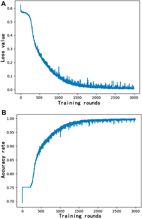
FIGURE 7. Results of 3,000 training rounds. (A) Loss rate function curve; (B) accuracy rate curve.

An identification result of pipeline leakage together with the corresponding model and the B-scan image are displayed in Figure 8. Obviously, the network proposed in this study can accurately distinguish pipelines, leakage areas and untargeted areas. Compared with given data labels, the accuracy of simulated training results reaches about 93%, implying that this classification network is well competent for underground oil pipeline classification and recognition. Furthermore, comparing the recognition results of the simulation data with their input labels, the calculated accuracy of the horizontal pipeline leakage identification, and longitudinal target location are 94.5% and 84.6%, respectively. Using the initial convolutional neural network without the attention module for training, the calculated accuracy rates of the horizontal pipeline leakage identification and longitudinal target location is 88.3% and 76.8%, respectively. The optimized network improves the accuracy rates of the horizontal pipeline leakage identification and longitudinal target location by 6.2% and 7.8%, respectively. It can be seen that the optimized networks with attention modules can greatly improve the recognition results.

FIGURE 8

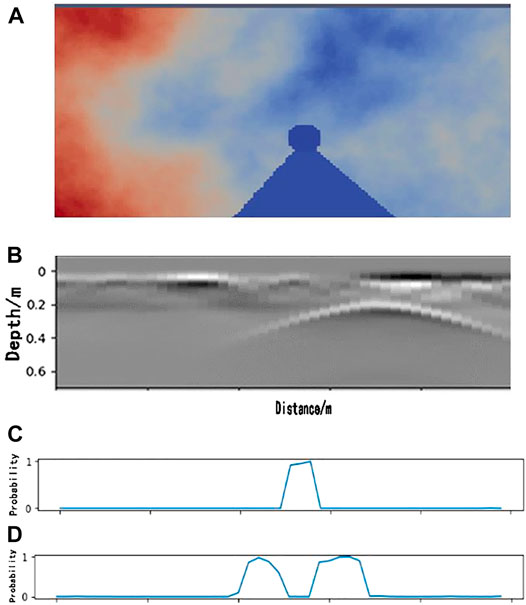
FIGURE 8. Classification network identification results. (A) Pipeline leakage model; (B) pipeline leakage B-scan diagram; (C) pipeline discrimination probability; (D) leak discrimination probability.

As for the judgments of depth and leakage area, the designed network can get results with an average accuracy rate of 95.1% (Figure 9A) and 96.4% (Figure 9B), respectively.

FIGURE 9

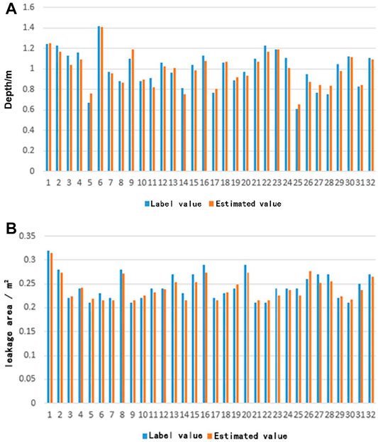
FIGURE 9. Results of pipeline depth. (A) and leakage area; (B) identification

Measured Results and Analysis

In order to verify the applicability of the underground target recognition method based on the attention mechanism to real data, we went to the Tahe Oilfield in Xinjiang to provide measured data support for a neural network. According to the prior knowledge obtained from simulation, the measured parameters of GPR are set as follows. The antenna is 250 Mhz, the time window is 100 ns, the sampling interval is 0.4 ns, and the antenna step is 0.05 m. With the aforementioned parameter settings, the effective detection depth is 3 m and the resolution is 0.2 m.

As shown in Figure 10, the experiment was mainly conducted in a desert environment with undulating topography. The soil within the detection depths is composed of gray-white fine sand and silt sand layers with a yellow-gray clay layer. The oil pipeline is buried in the soil to a depth of about 1–2 m. Considering the conditions of the test environment and oil pipeline laying, both longitudinal and horizontal detection lines were adopted. A horizontal line was set to collect relatively comprehensive information along the oil pipeline laying direction. The longitudinal line is perpendicular to the oil pipeline laying direction, which can supplement the detection of abnormal sites and extract the reflection characteristics of an oil pipeline.

FIGURE 10

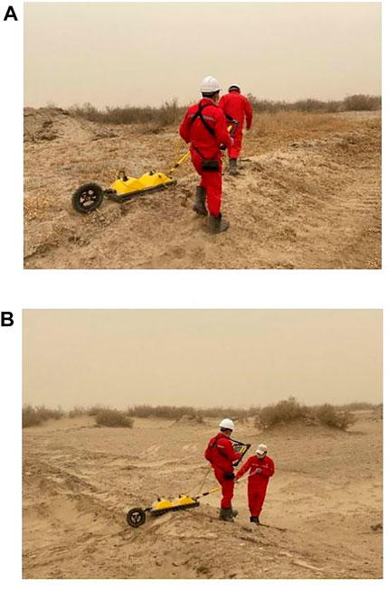
FIGURE 10. Measurements in different directions. (A) Horizontal detection line; (B) longitudinal detection line.

The actual detection area is roughly modeled in Figure 11A. As for the lack of leaking oil pipeline, simulated leakage points were set up along the oil pipeline line. As the cross-section of the simulating leakage model shown in Figure 11B, two 50 × 50 × 60 cm sandpits were excavated directly above the simulated leakage points and filled with water. These sandpits were backfilled and tamped after the natural infiltration of water. GPR was used for longitudinal and horizontal detections before and after simulating leakage. The different characteristics of reflected waves received by radar before and after the change of physical properties of the surrounding medium are analyzed from the obtained data.

FIGURE 11

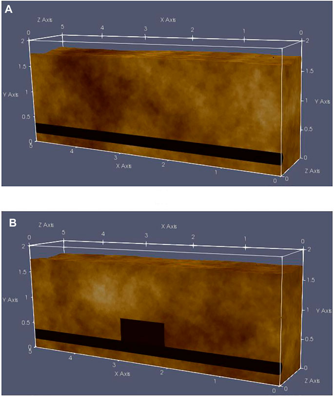
FIGURE 11. Cross-sectional models of actual oil pipeline detection (A) and simulated oil pipeline leakage area (B).

The experiment data are grouped according to the horizontal and longitudinal lines and input into the neural network for learning after being associated with their respective label data. This indicates that the network is running properly. Take the loss value function curve and accuracy curve of data from the horizontal line as examples. When training the network, Adam is selected by the optimizer, where the learning rate is 0.0001, the loss function is “categorical_crossentropy,” and the accuracy rate is “keras.metrics_accuracy.” After 500 rounds of training, namely 500 epochs, the loss value gradually decreases, while the accuracy rate gradually increases and approaches 1, as shown in Figure 12. The loss value and accuracy of the longitudinal line are similar to those of the horizontal line, indicating that the network is running properly.

FIGURE 12

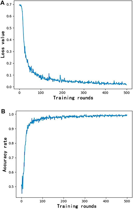
FIGURE 12. Results after 500 times of training with horizontal test data. (A) Loss rate function curve; (B) accuracy rate curve.

The measured data may output three cases, including oil pipeline, leakage and no target. Results are given in terms of the probability of each type being present at a certain location. In the aforementioned three cases, the case with the highest probability is output as the final recognition result. The discrimination time of artificial intelligence method for single GPR data is about 20 s, which is greatly improved compared with manual interpretation method. Notably, for the case that leakage and oil pipeline exist simultaneously, the output discrimination result of proposed network will be leakage, because the simulated leakage area is located above the oil pipeline.

Selecting a set of oil pipeline leakage identification results from horizontal detection data for further discussion. The cross-section of the experimental area is modeled in Figure 13A, and the identification result, as well as the B-scan image, are shown in Figure 13B. There are multiple echoes in the B-scan image (Figure 13B), which strongly interfere with the results of manual discrimination. Instead, thetraining results of the novel network in this study can be perfectly matched with the labeled experimental data. During the detection, marks were made at F1 and F2 to indicate the occurrence of leakage with the abscissa ranging from about 4.67 to 5.94 m. As marked with a red frame in Figure 13B, the proposed network gives the classification with the highest probability from 4.74 to 6.14 m, corresponding well to the marked area. This implies that our network can avoid distractions and output the results only representing targets of interest.

FIGURE 13

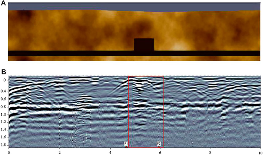
FIGURE 13. (A) Cross-section of simulated model for horizontal oil pipeline leakage detection. (B) Corresponding leakage identification results.

Similarly, a set of longitudinal oil pipeline leakage identification results is also chosen for analysis. The cross-section of the simulated experimental model and the result of the B-scan image after network identification are successively shown in Figure 14. The simulated leakage is marked from 5.4 to 6.2 m along X-coordinate, and an oil pipeline is marked at 14.8 m. After network training, the identified leakage section, represented by the red frame in Figure 14B, locates at 4.7 and 6.5 m on the horizontal axis, and the identified oil pipeline part, represented by the blue frame in Figure 14B , is 14.4–15 m. The output results are in good agreement with the given labels. In addition, there are some interferences at about 2 and 9.4 m in the B-scan image. However, our network does not take these interferences as target signals and the identification results exclude them from the targets of concern.

FIGURE 14

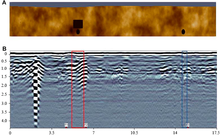
FIGURE 14. (A) Cross-section of simulated model for longitudinal oil pipeline leakage detection. (B) Identification results of simulated leakage and oil pipeline under normal working condition.

Comparing the identification results of the test data after network training with their input labels, the calculated accuracy rates of the horizontal oil pipeline leakage data and longitudinal target data are 92.3% and 84.4%, respectively. Using the initial convolutional neural network without the attention module for training, the calculated accuracy rates of the horizontal pipeline leakage identification and longitudinal target location are 86.9% and 77.5%, respectively. The optimized network improves the accuracy rates of the horizontal pipeline leakage identification and longitudinal target location by 5.4% and 6.9%, respectively. The optimized networks with the attention module help improve the recognition results. To sum up, the constructed network in this article can be well applied to the measured GPR data.

Conclusion

Through the optimized convolutional neural network based on the attention mechanism, the key information of the target of the underground oil pipeline can be identified. The simulation results show that after using the optimized new convolutional neural network, the accuracy rates of the leakage discrimination from horizontal data acquired along the oil pipeline and the classification of the target from longitudinal data acquired perpendicular to the oil pipeline are 94.5% and 84.6%, respectively. Compared with the original convolutional neural network without an attention mechanism, the corresponding accuracy rates are improved by 6.2% and 7.8%, respectively. Furthermore, the field measured results show that after using the optimized network, the accuracy rates of the leakage discrimination and the classification of the target are 92.3% and 84.4%, respectively. Compared with that of the conventional network, the accuracy rates of the leakage discrimination and the targets classification are improved by 5.4% and 6.9%, respectively. The research results show that the proposed network models are competent for the underground oil pipeline targets recognition with the simulated and measured data with high accuracy.

Data Availability Statement

The raw data supporting the conclusion of this article will be made available by the authors, without undue reservation.

Author Contributions

JL is responsible for the field experimental design, measured data acquisition, and article writing. DY is responsible for data processing, network construction, and article writing. CG is responsible for the experimental design. CJ is responsible for high quality data processing of measurement data. YJ is responsible for data processing. HS is responsible for the acquisition and processing of high quality simulation data. QZ is responsible for the overall design scheme.

Funding

This work was financially supported by fundings from the Sub-topics of National Key R&D Program (No. 2018YFC0603303), the Sichuan Science and Technology Program (Grant No. 2021YFH0057 and 2021YFG0369) and the SINOPEC Northwest Oil Field Company (No. 34400007-19-ZC0607-0234).

Conflict of Interest

CJ was employed by CNPC Logging Company Limited Tianjin Branch. HS was employed by SINOPEC Northwest Company.

The remaining authors declare that the research was conducted in the absence of any commercial or financial relationships that could be construed as a potential conflict of interest.

Publisher’s Note

All claims expressed in this article are solely those of the authors and do not necessarily represent those of their affiliated organizations or those of the publisher, the editors, and the reviewers. Any product that may be evaluated in this article, or claim that may be made by its manufacturer, is not guaranteed or endorsed by the publisher.

References

Cao, Zhenfeng., Yang, Shifu., Song, Shirong., and Zhou, Jian. (1996). Ground Penetrating Radar Data Processing Method and its Application[J]. Geology. Exploration 32 (01), 34–42. (in Chinese with English abstract).

Google Scholar

Chen, J., Wang, S., Liu, Z., and Guo, Y. (2018). Network-based Optimization Modeling of Manhole Setting for Pipeline Transportation. Transportation Res. E: logistics transportation Rev. 113, 38–55. doi:10.1016/j.tre.2018.01.010

CrossRef Full Text | Google Scholar

Hinton, G. E., and Salakhutdinov, R. R. (2006). Reducing the Dimensionality of Data with Neural Networks. science 313 (5786), 504–507. doi:10.1126/science.1127647

PubMed Abstract | CrossRef Full Text | Google Scholar

Hu, C., Wang, F., and Ai, C. (2021). Calculation of Average Reservoir Pore Pressure Based on Surface Displacement Using Image-To-Image Convolutional Neural Network Model. Front. Earth Sci. 9, 712681. doi:10.3389/feart.2021.712681

CrossRef Full Text | Google Scholar

Jia, L., Guo, C., Wang, F., and Zhang, J. (2007). The Summary of the Surface Ground Penetrating Radar Applied in Subsurface Investigation[J]. Prog. Geophys. 22 (02), 629–637. (in Chinese with English abstract). doi:10.3969/j.issn.1004-2903.2007.02.043

CrossRef Full Text | Google Scholar

Kang, M.-S., Kim, N., Lee, J. J., and An, Y.-K. (2020). Deep Learning-Based Automated Underground Cavity Detection Using Three-Dimensional Ground Penetrating Radar. Struct. Health Monit. 19 (1), 173–185. doi:10.1177/1475921719838081

CrossRef Full Text | Google Scholar

Kunihiko, F., and Sei, M. (1982). Neocognitron: A New Algorithm for Pattern Recognition Tolerant of Deformations and Shifts in Position[J]. Pattern Recognition 15 (6), 455–469.

Google Scholar

Lei, W., Hou, F., Xi, J., Tan, Q., Xu, M., Jiang, X., et al. (2019). Automatic Hyperbola Detection and Fitting in GPR B-Scan Image. Automation in Construction 106, 102839. doi:10.1016/j.autcon.2019.102839

CrossRef Full Text | Google Scholar

Lei, W., Luo, J., Hou, F., Xu, L., Wang, R., and Jiang, X. (2020). Underground Cylindrical Objects Detection and Diameter Identification in GPR B-Scans via the CNN-LSTM Framework. Electronics 9 (11), 1804. doi:10.3390/electronics9111804

CrossRef Full Text | Google Scholar

Li, W., Cui, X., Guo, L., Chen, J., Chen, X., and Cao, X. (2016). Tree Root Automatic Recognition in Ground-Penetrating Radar Profiles Based on Randomized Hough Transform. Remote Sensing 8 (5), 430. doi:10.3390/rs8050430

CrossRef Full Text | Google Scholar

Liang, S., Jianlin, W., and Liqiang, Z. (2010). Analysis on Detectable Leakage Ratio of Liquid Pipeline by Negative Pressure Wave Method. Acta Petrolei Sinica 31 (4), 654–658. doi:10.7623/syxb201004026

CrossRef Full Text | Google Scholar

Liu, Q., Zhang, N., Yang, W., Wang, S., Cui, Z., Chen, X., et al. (2017). “A Review of Image Recognition with Deep Convolutional Neural Network,” in International Conference on Intelligent Computing, Liverpool, UK, August 7–10, 2017 69–80. doi:10.1007/978-3-319-63309-1_7

CrossRef Full Text | Google Scholar

Lu, H., and Zhang, Q. (2016). Application of Deep Convolutional Neural Network in Computer Vision[J]. J. Data Acquisition Process. 31 (01), 1–17. (in Chinese with English abstract). doi:10.16337/j.1004-9037.2016.01.001

CrossRef Full Text | Google Scholar

Peplinski, N. R., Ulaby, F. T., and Dobson, M. C. (1995). Dielectric Properties of Soils in the 0.3-1.3-GHz Range. IEEE Trans. Geosci. Remote Sensing 33 (3), 803–807. doi:10.1109/36.387598

CrossRef Full Text | Google Scholar

Sagnard, F., and Tarel, J.-P. (2016). Template-matching Based Detection of Hyperbolas in Ground-Penetrating Radargrams for Buried Utilities. J. Geophys. Eng. 13 (4), 491–504. doi:10.1088/1742-2132/13/4/491

CrossRef Full Text | Google Scholar

Tang, J., Fan, B., Xiao, L., Tian, S., Zhang, F., Zhang, F., et al. (2020). A New Ensemble Machine-Learning Framework for Searching Sweet Spots in Shale Reservoirs[J]. SPE J. 26 (1), 482–497. doi:10.2118/204224-pa

CrossRef Full Text | Google Scholar

Terrasse, G., Nicolas, J. M., Trouvé, E., and Drouet, É. (2016). “Automatic Localization of Gas Pipes from GPR Imagery[C],” in 2016 24th European Signal Processing Conference (EUSIPCO), Budapest, Hungary, August 29–September 2, 2016, 2395–2399.

Google Scholar

Vargas, R., Mosavi, A., and Ruiz, R. (2017). Deep Learning: A Review[J]. Adv. Intell. Syst. Comput. 5, 1–11.

Google Scholar

Wang, L., Wang, H., and Xiong, M. (2014). Technical Analysis and Research Suggestions for Long-Distance Oil Pipeline Leakage Monitoring. Oil Gas Storage and Transportation 33 (11), 1198–1201. doi:10.6047/j.issn.1000-8241.2014.11.010

CrossRef Full Text | Google Scholar

Wang, S., and Chen, S. (2019). Insights to Fracture Stimulation Design in Unconventional Reservoirs Based on Machine Learning Modeling. J. Pet. Sci. Eng. 174, 682–695. doi:10.1016/j.petrol.2018.11.076

CrossRef Full Text | Google Scholar

Wanjun, Liu., Xuejian, Liang., and Haicheng, Qu. (2016). Learning Performance of Convolutional Neural Networks with Different Pooling Models[J]. J. Image Graphics 21 (9), 1178–1190. (in Chinese with English abstract). doi:10.11834/jig.20160907

CrossRef Full Text | Google Scholar

Windsor, C. G., Capineri, L., and Falorni, P. (2013). A Data Pair-Labeled Generalized Hough Transform for Radar Location of Buried Objects[J]. IEEE Geosci. Remote Sensing Lett. 11 (1), 124–127. doi:10.1109/LGRS.2013.2248119

CrossRef Full Text | Google Scholar

Woo, S., Park, J., Lee, J.-Y., and Kweon, I. S. (2018). “CBAM: Convolutional Block Attention Module,” in Proceedings of the European conference on computer vision (ECCV), Munich, German, September 8–14, 2018, 3–19. doi:10.1007/978-3-030-01234-2_1

CrossRef Full Text | Google Scholar

Xiong, H., Kim, C., and Fu, J. (2020). “A Data-Driven Approach to Forecasting Production with Applications to Multiple Shale Plays[C],” in SPE Improved Oil Recovery Conference, Tulsa, USA, August 31–September 4, 2020 (Society of Petroleum Engineers (SPE)).

Google Scholar

Yang, D., Hou, N., Lu, J., and Ji, D. (2021). Novel Leakage Detection by Ensemble 1DCNN-VAPSO-SVM in Oil and Gas Pipeline Systems. Appl. Soft Comput., 115, 108212. doi:10.1016/j.asoc.2021.108212

CrossRef Full Text | Google Scholar

Zhao, Y. Z., Su, Y. L., Hou, X. Y., and Hong, M. H. (2021). Directional Sliding of Water: Biomimetic Snake Scale Surfaces. Opto-Electronic Adv. 4 (4), 04210008. doi:10.29026/oea.2021.210008

CrossRef Full Text | Google Scholar

Zhou, Z., Zhang, J., Huang, X., and Guo, X. (2019). Experimental Study on Distributed Optical-Fiber cable for High-Pressure Buried Natural Gas Pipeline Leakage Monitoring. Opt. Fiber Tech. 53, 102028. doi:10.1016/j.yofte.2019.102028

CrossRef Full Text | Google Scholar