Dynamic strain anomalies detection at Stromboli before 2019 vulcanian explosions using machine learning

Identifying and characterizing the dynamics of explosive activity is impelling to build tools for hazard assessment at open-conduit volcanoes: machine learning techniques are now a feasible choice. During the summer of 2019, Stromboli experienced two paroxysmal eruptions that occurred in two different volcanic phases, which gave us the possibility to conceive and test an early-warning algorithm on a real use case: the paroxysm on July, 3 was clearly preceded by smaller and less perceptible changes in the volcano dynamics, while the second paroxysm, on August 28 concluded the eruptive phase. Among the changes observed in the weeks preceding the July paroxysm one of the most significant is represented by the shape variation of the ordinary minor explosions, filtered in the very long period (VLP 2–50 s) band, recorded by the Sacks-Evertson strainmeter installed near the village of Stromboli. Starting from these observations, the usage of two independent methods (an unsupervised machine learning strategy and a cross-correlation algorithm) to classify strain transients falling in the ultra long period (ULP 50–200 s) frequency band, allowed us to validate the robustness of the approach. This classification leads us to establish a link between VLP and ULP shape variation forms and volcanic activity, especially related to the unforeseen 3 July 2019 paroxysm. Previous warning times used to precede paroxysms at Stromboli are of a few minutes only. For paroxysmal events occurring outside any long-lasting eruption, the initial success of our approach, although applied only to the few available examples, could permit us to anticipate this time to several days by detecting medium-term strain anomalies: this could be crucial for risk mitigation by prohibiting access to the summit. Our innovative analysis of dynamic strain may be used to provide an early-warning system also on other open conduit active volcanoes.

1 Introduction

The current state of art about the development of early warning systems in volcanic areas reports robust results only for short-term precursors at open-conduit volcanoes. In a recent work Dempsey et al. (2020), use an algorithm on the Whakaari/White Island volcano capable of finding a 17 h warning prior to the fatal 2019 eruption, with a peak of the warning occurring 4 h prior to that event. Another example of an early-warning system, based on an unsupervised algorithm capable of providing automatic notifications of eruptions to Government agencies, has been developed by Ripepe et al. (2018) for Mt. Etna, Italy: based on the analysis of infrasonic signals, it provides high success rates on upcoming eruptions characterized by a smooth increase in the amplitude of both seismic and infrasonic signals hours before, delivering pre alert notification about 1 h before the occurrence of the eruptive onset. On the same volcano, Spampinato et al. (2019) design a multi-station warning system based on the classification of patterns of the volcanic tremor, by using Self-Organizing Maps (SOM) and fuzzy clustering. The classifier forecasts hours before in hindsight patterns associated with fast-rising magma (typical of lava fountains) as well as a relatively long lead time of the outburst (lava flows from eruptive fractures).

Steadily erupting basaltic volcanoes produce Strombolian type outbursts, rarer fire fountains, effusive activity and paroxysmal explosions, occurring irregularly every several years (Bevilacqua et al., 2020; Mattia et al., 2021). The latter represent a major hazard owing to their sudden occurrence and wide impact. The origin of these unforecasted blasts remains poorly understood, as well as their relationship with the usual explosive activity and the effusive eruptions. Identifying their triggering mechanism and potential precursors is of outmost importance for both volcano research and civil defense purposes. Stromboli volcano is one of the best sites for studying basaltic explosive paroxysms. It is an active, open-conduit strato-volcano, located in the northernmost area of the Aeolian Archipelago, Southern Italy, characterized by a moderately persistent volcanic activity with a paucity of deformation episodes: hence it has always been a candidate volcano as a natural laboratory for researchers investigating eruptive precursors on open-conduit volcanoes. In the past, Pino et al. (2011) reported on the first detection of seismic signals precursory to a paroxysm on 5 April 2003 at Stromboli. This strong event was preceded by 25 h of seismic tremor variation, broadly coincident with strong geochemical anomalies in crater plume emissions. Newly, Di Lieto et al. (2020) and Giudicepietro et al. (2020) have analyzed the signals of a borehole strainmeter installed on the island, obtaining automatic triggers 10 and 7.5 min before the July 3 and the 28 August 2019 paroxysms, respectively. These results highlight very short-term precursors of paroxysmal activity and provide a first valuable evidence for the development of an early warning system for paroxysmal explosions based on strainmeter measurements.

Explosive activity, with several hundreds of events per day (Martini et al., 2007) at intervals ranging from about 3 to 15 min, dominates Stromboli’s dynamics. Each explosion generates a seismic signal with high and low frequency content, the latter characterized by periods of 3 s or more (Neuberg et al., 1994), like that observed at other open-conduit active volcanoes (see, e.g., Nishimura et al., 2000; Aster et al., 2003). Higher frequencies have been explained as ground-coupled airwaves produced during an explosion (Braun and Ripepe, 1993), while the lower frequency content is generally associated with long- (LPs) and very long-period events (VLPs). These last phenomena are related to volume changes inside the conduit, caused by mass transport toward the surface (Chouet et al., 2008). Statistical analyses of LPs and VLPs were conducted on a data set from Stromboli volcano, for which the recorded LP-VLP transients are associated with the recurrent summit explosions, characteristic of Strombolian activity (Cauchie et al., 2015). As opposed to these highly frequent explosions, deformation episodes occur less often: one of the most important occurred between December 1994 and March 1995, when a significant variation in tilt data was observed before a seismic event with magnitude 3.7, due to the activation of a NE-SW striking structure, accompanied by magmatic fluid injection (Buonaccorso, 1998). During 2000, a significant tilt and GPS variation was recorded (Mattia et al., 2008). Here the 2002–2003 eruption and its paroxysm are missing The 2007 paroxysmal eruption occurred during an effusive phase and was characterized by a ten times greater initial volume emission, followed by the largest most recent deformation (Calvari et al., 2005, 2010). Strong strain variations, occurring minutes before major and paroxysmal eruptions, were revealed by dilatometer data analysis (Bonaccorso et al., 2012; Giudicepietro et al., 2020; Di Lieto et al., 2020). Several authors have shown that the dynamics of Stromboli is strongly correlated with an observed change in shape of VLPs (see, e.g., Braun and Ripepe, 1993; Chouet et al., 2003 and, more recently, Giudicepietro et al., 2020). VLPs due to volcanic activity are interpreted as characteristic of their source, since the waveforms are less prone to be modified by the topography or by structural heterogeneity within or near the conduct. Possible source mechanisms for various volcanoes in the world include deflations and inflations of magma chambers (Nishimura et al., 2000), volumetric sources (Kumagai et al., 2001) and volume changes (Julian et al., 1997). The VLP activity at Stromboli volcano can be explained as caused by the rapid expansion of a gas slug which nucleates within the magma in the conduit (Chouet et al., 2003). During this normal activity, the gas slugs are free to nucleate at any given point in the conduit due to the homogeneity of the magma, characterized by a low viscosity and a high permeability (La Spina et al., 2017): polarization analysis of the VLPs recorded by a 3-component seismic station shows a dispersion of azimuth and incidence angles during the usual volcanic activity (Giudicepietro et al., 2020). Just before paroxysmal eruptions, however, VLP azimuth and incidence angle dispersion disappears, suggesting a decrease of the permeability of the magma stored in uppermost portion of the feeding system, which in turn could be caused by an increase in its viscosity, due to cooling of the melt and incipient crystallization (Mattia et al., 2021).

Previous seismic surveys conducted using broadband seismometers and focusing on the VLP frequency content of the recorded explosions found that VLP shapes tend to cluster in families of similar events: a clustering analysis detected two different families of VLPs with well-defined shapes generated by explosions occurring at two different active vents (Chouet et al., 1999). Earlier, Ripepe et al. (1993) had suggested that these families are mostly linked to gas pressure fluctuations rather than to crater geometry. Depending on the currently active vents and the overall explosive activity, however, more than two families can be found in volcano dynamics (Kirchdörfer, 1999).

During the summer of 2019, Stromboli experienced two paroxysmal eruptions; the first in July, the second in August. They have been subject matter of studies using geological, geophysical and geochemical approaches (Bevilacqua et al., 2020; Inguaggiato et al., 2020; Corradino et al., 2021; Giordano and De Astis, 2021; Mattia et al., 2021; Métrich et al., 2021; Viccaro et al., 2021). Although their energy release was comparable (Di Lieto et al., 2020; Giudicepietro et al., 2020), explosions occurred in two different volcanic phases: the paroxysm on July 3 was only preceded, in the previous weeks, by two volcano-tectonic seismic events and a major explosion with a smaller and less perceptible changes in the volcano dynamics; the second paroxysm, on August 28, occurred, similarly to 2007 paroxysms (Di Lieto et al., 2020), during ongoing effusive and explosive activity and marked the end of the eruptive phase that began with the previous paroxysmal event (Di Lieto et al., 2020; Giudicepietro et al., 2020; Andronico et al., 2021). The 2019 paroxysmal events have been described by Giudicepietro et al. (2020) and Di Lieto et al. (2020) in relation to the pressure source and their short term (minutes before event) geophysical precursors.

A crucial challenge for the scientific community is to enlarge the current hourly temporal window of very intense explosion (major explosions and paroxysms) foreseeability to days or even weeks before the event, especially for those events occurring outside any long-lasting eruption, when the volcano summit may be open to visitors. In the past, machine learning methodologies were applied to characterize volcanic regimes and to define short-to medium-term forecasts (Carniel and Di Cecca, 1999; Jaquet and Carniel, 2001; Jaquet and Carniel, 2003; Carniel et al., 2006a; Carniel et al., 2006b; Telesca et al., 2010; Carniel, 2014).

Among the changes observed in the weeks preceding the July explosion, as found by Mattia et al. (2021), one of the most significant is represented by the shape variation of the explosions, filtered in the VLP band, as recorded by the Sacks-Evertson strainmeter installed near the village of Stromboli. Starting from these two observations, the original use of the strain data allowed us to extend the usual seismic VLP (2–50 s) frequency band used in previous works, by including also the ultra long-period (ULP - 50–200 s) band using two independent methods in order to classify events falling in the VLP-ULP frequency bands: a modified version of the Green-Neuberg VLP-ULP classification algorithm (Green and Neuberg, 2006), and an unsupervised machine learning strategy, namely the self-organizing map (Kohonen et al., 1996; Kohonen, 2001). The results of the two methodologies were compared to highlight their robustness.

2 Materials and methods

The data recorded from the borehole strainmeter carry several pieces of information, due to the intrinsic capability of the instrument of recording high precision data within a wide frequency range, being able to record the static and dynamic deformations. This information is difficult to interpret because of unclear knowledge of source processes and the large amount of data stored. For the former problem, the researchers are proposing innovative models (e.g., for VLPs interpretation see Legrand and Perton, 2022); about the latter, machine learning algorithms can play an important role in discovering the presence of patterns, otherwise hidden, among data: in the past, data analysis and machine learning algorithms have already been successfully applied to seismic data, allowing to found families of self-similar events with a common origin (see, e.g., Green and Neuberg, 2006), and nowadays more applications have been developed, some specifically regarding Stromboli (Bergen et al., 2019; Seydoux et al., 2020).

In the present work, we developed a method capable of automatically picking volcanic events belonging to both VLP (strain data filtered between 2 and 50 s) and ULP (2–200 s) bands, and classifying them in families based on event shape changes, using two concurrent algorithms, in order to mutually verify their outcomes: a cross-correlation among VLP/ULP signals and an unsupervised neural strategy. Both methods were applied on data recorded throughout the year 2019 to validate the algorithms. Then the neural network method was extended to a wider (May 2018-December 2020) period to verify that families found in a narrower time interval were still present. We tried, then, to associate families with volcanic activity, finally proposing a conceptual model capable of explaining the changes found.

2.1 Instrumental focus

Stromboli volcano monitoring system has been improved, after the 2003 paroxysmal event, with two borehole Sacks-Evertson dilatometers (San Vincenzo Observatory, SVO, and Timpone del Fuoco, TDF, in Figure 1), installed during 2006, by Italian Civil Protection Department, INGV and Università degli Studi di Salerno (Italy), in cooperation with Carnegie Institution of Washington D.C. (United States). The radial distances of SVO and TDF strainmeters are about 2.5 km north-east and 1.5 km west from the main eruptive vents, respectively. Data recorded by the SVO strainmeter are sampled at 1 sample per second (sps) and exhibit a very high signal to noise ratio (SNR), which made it a valuable help in understanding the volcano dynamics and changes occurring in the shallow plumbing system of Stromboli volcano. TDF data are affected by a weak coupling of the instrument with the surrounding rocks. Moreover, the instrument was not in operation during 2019, so the analyses in the current paper have been carried out on data recorded by SVO only.

FIGURE 1

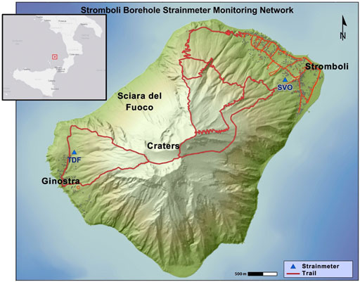
FIGURE 1. Location of Stromboli island and sites of the strainmeter network (from Di Lieto et al., 2020). The trails are reported to highlight the scarce presence of the escape routes.

A Sacks-Evertson strainmeter is a stainless-steel tube (7 cm in diameter and 4 m in length) filled with degassed silicone oil which is able to observe a broad class of behaviors (see Figure 2 in Silver et al., 1999). Its output is obtained by a hydro-mechanical amplification system, measuring volumetric changes through the use of a small bellows, whose changing length is measured by a linear variable differential transformer (LVDT). It measures a single component of volumetric change in the earth near a deforming zone, without any clue about the direction of the principal strains. Once installed in the borehole, strainmeters are cemented with an expansive grout to couple them with the surrounding rocks and cannot be recovered, so they must be calibrated in situ: SVO strainmeter shows a sensitivity of 10⁻¹¹ per digital count (Di Lieto et al., 2020).

FIGURE 2

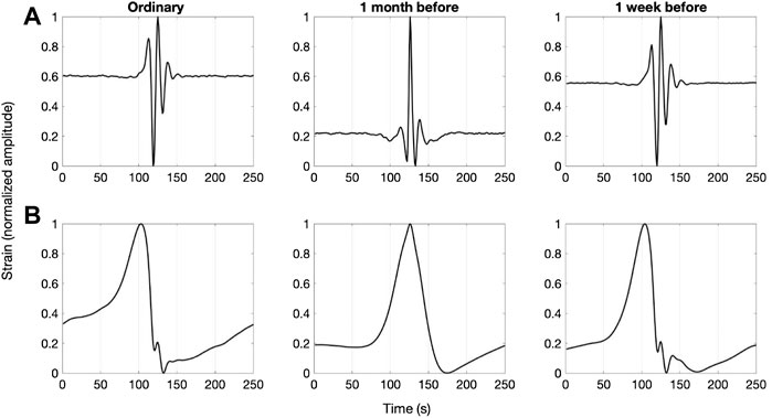
FIGURE 2. (A) Normalized stacked VLP waveforms for three time periods of the whole year 2019: “ordinary” volcano activity present before (from January to May) and after (from July to December) 2019 eruptive activity, 1 month and 1 week before 3 July paroxysm. (B) Normalized stacked ULP waveforms for the same three time periods.

The choice to focus our analysis on the frequency band of the dynamic strain is justified by the intrinsic instrumental characteristics. Due to a linear from zero (DC or static) to sub-acoustic frequencies instrumental response, strainmeters represent a bridge between seismological and geodetic measurements. Furuya and Fukudome (1986) investigated the response of a borehole volume strainmeter to various kinds of disturbances, including seismic waves, and determined that for P-, S- and Rayleigh waves, and Earth tides, the sensitivities are very similar. From a comparison among different seismometers and strainmeters, it was found that borehole strainmeters are more suitable for recording seismic waves with respect to other kinds of strainmeters (Barbour and Agnew, 2012). Simultaneous recordings of strain and three-component seismic velocity suggest that strainmeters detect the dilatational energy for seismic radiation at earth-noise levels for periods in the range 0.05–20 Hz (Borcherdt et al., 1989). The dynamic strains, associated with seismic waves, may play a significant role in earthquake triggering, earthquake damage, ground failure and hydrological and magmatic changes (Gomberg and Agnew, 1996).

2.2 Data analysis: Detection and classification of VLP-ULP volcanic signals

In this paper we have analyzed the strain signals collected during the year 2019. A quantitative classification of events filtered in the two different frequency bands recorded by the Sacks-Evertson strainmeter has been carried out using two different techniques: a cross-correlation cluster analysis and a self-organized map (SOM) neural network technique. For the resulting catalog, we find an automated procedure to cluster events and examine the temporal variations of their shapes, in order to correlate the families found with specific volcanic activities.

Thanks to its high signal-to-noise ratio (SNR), the SVO strainmeter is capable of recording strain changes characterized by low environmental noise levels. An automated detection algorithm has been used in order to find VLPs during the Jan-December 2019 period. Firstly, data have been pre-processed in order to remove any spurious artifacts like valves opening/closing that cause highly energetic spikes which could affect the subsequent data analysis. The pre-processed signal has been bandpass filtered in two different frequency ranges using a Butterworth three-pole digital filter: the band 0.005–0.5 Hz (ULP iteration), and the band 0.02–0.5 Hz (VLP iteration).

In order to automate the algorithm, we used a short-term amplitude average (STA) versus long-term amplitude average (LTA; Allen, 1978) ratio: the STA/LTA algorithm was capable of detecting the vast majority of the events in the analyzed time-frame, lacking in performance only when bad weather or adverse sea conditions occurred, since the frequencies characterizing these occurrences fall within the same range of the VLPs (or ULPs). By considering the frequency band of the filtered signals as well as the typical duration of the events recorded at the strainmeter, window sizes of 12 and 3,600 s (or 15 and 5,000 for ULPs) were used to determine the values of STA and LTA, respectively. This allowed us to find 60,826 VLPs and 57,826 ULPs in the inspected period. A preliminary study of the strain data frequency content of the selected time windows influenced the filter band choice made for the time series analyzed. From a visual inspection of the strain data, we selected VLPs recorded in the 0.02–0.2 Hz frequency band with a high signal-to-noise ratio in a time window 250s long. Three time periods, characterized by different volcanic states, were found: the first period from June, 1 to June, 25 (“1 month before” in Figure 2), the second one from June, 25 to July, 3 (“1 week before” in Figure 2), pointing the remaining events as “ordinary”. These VLPs were stacked with a normalized amplitude obtained by rescaling the range of the data to the interval [0,1] (Figure 2A). Using the same time window and procedure, data filtered in the 50–200 s frequency band have been stacked in order to look for the presence of ULP transients. The ULP stacked waveforms concomitant with VLP ones show a repetitive and stationary trend over the whole year (Figure 2B). Note that, by using a visual inspection, no differences are detectable between “ordinary” and “1 week before” events.

VLP and ULP detection is strongly influenced by adverse weather and sea conditions. The number of detected events changes substantially during bad weather periods (rough sea, passage of high/low pressure fronts, severe thunderstorms), because of lower SNR ratio (see panel “a” of Figure 5 in Mattia et al., 2021, in which bad weather periods - lasting several days - are characterized by transients overwhelming typical VLP amplitudes) and does not allow clear automated detection of all the explosive events occurring at the active vents. It is known that much of the long-period spectral energy is due to ocean microseisms (OMS) (Braun, 2008).

2.2.1 Cross correlation analysis

Starting with the catalog of VLP signals obtained from the previous section, we quantified the similarity of shape of the events. In order to do so, we used a revised version of the algorithm by Green and Neuberg (2006), applied to seismic data, on each pair of events in the catalog. The cross-correlation (CC) function

$r_{xy}\left(i,i-l\right)=\frac{{{\displaystyle \sum }}_{i=1}^n\left(x_i-\underset{¯}{x}\right)\left(y_{i-l}-\underset{¯}{y}\right)}{\sqrt{{{\displaystyle \sum }}_{i=1}^n{\left(x_i-\underset{¯}{x}\right)}^2}\sqrt{{{\displaystyle \sum }}_{i=1}^n{\left(y_{i-l}-\underset{¯}{y}\right)}^2}}(1)$

returns an index of the similarity in shape of two waveforms, ignoring their relative amplitude. Each event lasts n samples: using the mean length of the trigger size and sampling details discussed above, we chose an equal length of 151 samples for each event, which is slightly larger than the maximum length of the events found in the catalogue, the middle point containing the maximum of the modulus of the event time window. In Eq. 1, we represent with x and y two different VLPs belonging to the catalog, each containing n samples: x_i represents the ith sample and y_i-l is the (i-l)th sample of the first and second event, respectively, while l is the lag between the two signals (l=0, being the complete overlap of the signals, has been chosen here). Underbar items represent the mean value of the signals. According to the Big-O notation (Black, 1998), a cross-correlation algorithm among N events, each lasting M samples, has a computational complexity of O(N² x M²) - or O(N² x M) when the fast Fourier transform (FFT) based cross-correlation is chosen, since in the frequency domain the sliding dot product becomes a mere multiplication. We have chosen to simplify the process by limiting the sliding window to just one value, by selecting the main peak of each event and centering it in the central point of the event window.

The classification method described above is capable of clustering strain transients into groups with similar waveforms. A threshold correlation coefficient, C, is needed to separate events falling in a specific family from those belonging to different families; this results in a trade-off between robustness of the method and the number of families found. For a low C-value, transients which slightly differ from each other will fall in the same family, generating a small number of families and unifying many events which potentially belong to different families. On the other hand, a high C-value results in a higher number of families, most of which may be populated by a small number of events; we require a minimum number of events K per family to minimize this issue. Rarest events are classified by the algorithm as characterized by slightly different phases, showing the same shape as the most frequent ones.

For a chosen C-value, the events whose mutual cross-correlation value exceeds the C threshold are clustered together and stacked, determining the master waveforms of each group. The process is iterated once these events are removed from the matrix and grouped in a new family. Finally, the master waveforms are cross-correlated in turn with the events not clustered yet, using the same C-value to classify a broader group of events.

2.2.2 Self-organizing map analysis

We apply an unsupervised neural strategy to cluster the N=60,826 events triggered by the automated STA/LTA algorithm (M-dimensional vectors M=151) in the band 2–50 s, and the N=57,826 events triggered in the band 2–200 s.

Among the unsupervised machine learning approaches, the Self-Organizing Map (SOM) (Kohonen et al., 1996; Kohonen, 2001) is widely used for clustering and visualization of large data sets of high dimensional data (it scales only linearly with the size of the dataset) and, moreover, it can be implemented in an on-line learning manner (Deng and Kasabov, 2003). The original motivation of the SOM research was actually an attempt to mimic aspects of self-organization seen in the somatotopic and abstract feature maps found in the biological central nervous systems (Kohonen, 2001).

The SOM carries out a nonlinear mapping of all observed data onto a two-dimensional map. The mapping preserves the most important topological and metric relationships of the data. It has proven to be an efficient tool for data-exploration tasks in a wide range of applications in various domains (Kohonen, 2008; Vellido et al., 2020), including speech recognition, image data compression, robot control, pattern recognition, medical diagnosis, categorization of galaxies (Naim et al., 1997) and massive document collections (Kohonen et al., 2000; Lagus et al., 2004). SOMs have already been applied, in different contexts, also to seismic data sets (Musil and Plešinger, 1996; Esposito et al., 2006; Esposito et al., 2008; Essenreiter et al., 2001; De Matos et al., 2007; Carniel et al., 2013a; Di Luccio et al., 2021). A hierarchical clustering was applied to results of SOM tremor analysis at Ruapehu (Carniel et al., 2013b) and Tongariro (Jolly et al., 2014) in New Zealand. A review of SOM and other machine learning strategies in volcanology can be found in Carniel and Guzmán (2020).

As with classical feed-forward networks, learning in SOMs is accomplished by adjusting the weights of the connections between grid units (neurons or nodes) and input units. In contrast to supervised feed-forward nets, SOMs learn in an unsupervised manner, guaranteeing minimal bias from the investigator. The SOM learning algorithm is such that, after learning, the final projection of the data on the SOM grid reveals some underlying structure in the data. One of the reasons for using SOM for, data exploration is to benefit from that topological structure when interpreting the data.

A major drawback of some clustering algorithms, such as for example the common k-mean algorithm, is that they are computationally intensive, especially when the size N of the training set grows. In most classical clustering approaches, every data item must be compared with all others, perhaps re-iteratively. For large masses of data this is obviously no longer efficient. Conversely, the SOM learning algorithm is easily and effectively applicable to large data sets (Kohonen, 2008) since the SOM computational complexity scales linearly with the number of data samples (and it does not require huge amounts of memory, only the prototype vectors and the current training vector).

The SOM map consists of a regular grid of processing units known as “neurons” or “nodes.” We use a hexagonal grid, in particular, a local hexagonal structure and a global sheet map. A prototype (also called a code vector) is associated with each node. The learning process of the map attempts to represent all the available data with optimal accuracy by using a restricted set of nodes. At the same time the nodes become ordered on the grid so that similar prototypes are associated with nodes close to one another and dissimilar prototypes with nodes far from one another. The whole dataset is presented, in random order, to the network during the learning strategy.

In the basic iterative and sequential SOM algorithm, at each iteration a single input vector is presented to the map. The winning node, i.e., the best matching unit (BMU), is identified (competitive aspect) and the prototype of the winning node is updated together with the prototypes of the neighborhood nodes (cooperative aspect).

At each iteration t, a feature input vector x(t) is extracted and the winner index c, i.e., the BMU of the input vector, is identified by the condition:

$\forall i, \left|x\left(t\right)-m_c\left(t\right) \right|\le \left| x\left(t\right)-m_i\left(t\right)\right|(2)$

where $x\left(t\right)$ is the feature vector of the signal extracted at step t, and $m_i\left(t\right)$ is the prototype of node i. After that, all prototypes in the neighborhood are updated by the equation

$m_i(t+1)=m_i\left(t\right)+h_{ci }(x\left(t\right)-m_i\left(t\right)) \left(3\right)$

Here $h_{ci}$ is the “neighborhood function,” a decreasing function of the distance between the ith and cth nodes on the map grid. As neighborhood function it is often used the Gaussian expressed as:

$h_{ci}\left(t\right)={\alpha }_{t }exp[\hspace{0.17em}-\hspace{0.17em}d{(c,i)}^2/ 2 r_t^2](4)$

where learning rate ${\alpha }_t$ is a monotonically decreasing scalar function of t, $d(c,i)$ is the geometric distance between the nodes c and i in the grid, and the neighborhood radius $r_t$ is another monotonically decreasing function of t. The exact mathematical form of $r_t$ is not crucial, as long as the value of $r_t$ is fairly large (e.g., on the order of half of the width of the grid) at the outset, and decreases to a value that is a fraction of the initial value, when a rough order of the models has been achieved (Kohonen, 2008).

3 Results

3.1 Cross-correlation results

The CC algorithm tries to best accommodate in a matrix all the events in the catalog. Due to its intrinsic behavior based on a given threshold, however, not all the events will be arranged within families. We tried different combinations of C- and K-values: as expected, the more the value of C is lowered, the more the algorithm classifies events which slightly differ from each other in larger groups; on the other hand, an increase in the C-value scatters waveforms in a higher number of less-populated families, most of which contain events whose waveforms are extremely similar in shape. At the same time, in order to avoid very low-populated families, we chose accordingly an appropriate K-value. Hence, we chose the two pairs of C- and K-values which give the best trade-off between the highest possible C along with a realistic number of families. Using C = 0.82 and K = 100 for the VLP iteration and C = 0.82 and K =150 for the ULP iteration, we build two cross-correlation matrices (Figures 3A,B). To check their mutual similarity, master waveforms have been cross-correlated with each other, obtaining a maximum correlation coefficient matrix of size n x n, n being the number of families found during the iteration: in this way we were able to verify visually the similarity between families. The choice of families with a mutual CC value above the given threshold of 0.82 and which had similar shape characteristics as confirmed by a visual inspection, allowed us to confirm that clusters of similar waveforms could be grouped together.

FIGURE 3

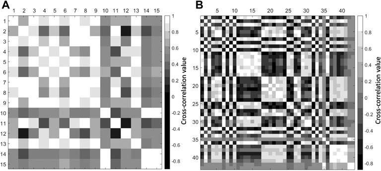
FIGURE 3. Cross-correlation matrices for (A) VLP and (B) ULP iterations. The matrices are 15×15 and 43×43 wide, respectively: the families found by the CC algorithm are reported on the x- and y-axes, while the blocks have a color associated with the mutual cross-correlation value. Lighter colors represent a higher degree of similarity.

The master waveforms found have their coherent signals added while the random noise contained in the generating events cancels out, allowing cross-correlation with the events not yet cataloged, using the same C-value previously used for VLP and ULP iterations. This last step has allowed us finally to generate temporal histograms of a much higher number of noisy events belonging to each family found in the previous step: in Figures 4A,B the histograms are shown.

FIGURE 4

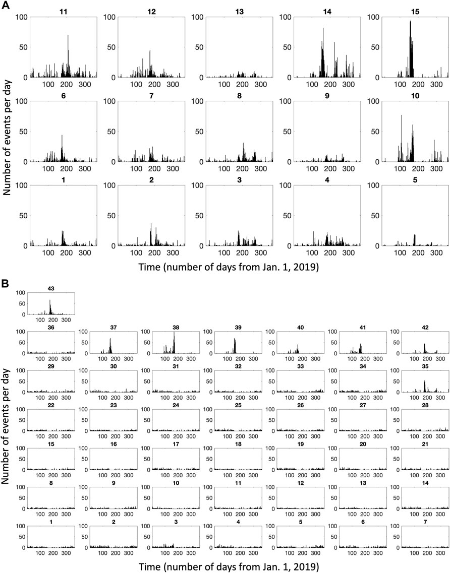
FIGURE 4. Temporal Histograms of cumulative number of events per day belonging to the ith family determined by the CC algorithm (A) events found by the VLP iteration (B) events found by the ULP iteration. The horizontal axis of the histograms indicates the time in 2019 Julian day.

We found a total of 15 and 43 families from the VLP and ULP iterations respectively, (Figures 5A,B), where the waveforms are determined as the stacking of the events whose mutual CC exceeded the chosen thresholds C: the total number of events belonging to each family in both iterations, depicted in Figures 4A,B, show each group exceeding the K-value chosen for the iteration.

FIGURE 5

FIGURE 5. Normalized stacked waveforms belonging to the ith family determined by the CC algorithm (A) families found by the VLP iteration (B) families found by the ULP iteration. The horizontal axis indicates time in seconds.

3.2 Self-organizing map results

A SOM strategy is used to project all the available N events in a SOM topographic map. In the preprocessing stage, for each of the N 151-dimensional vectors, in order to get a compact representation of the input data, we extract 22 features, which are given as input to the SOM learning algorithm, namely the maximum and minimum values of the normalized vectors and the first 20 principal components (extracted with linear Principal Components Analysis - PCA). Application of the SOM technique to our dataset, composed of N events, yields the maps illustrated in Figure 6. A SOM map with 5x5 units or nodes, each displayed as a hexagon, is used for clustering the VLP dataset. Given the higher heterogeneity of ULP data (more influenced by bad weather) we use a larger SOM map (with 8x8 units) to visualize the ULP dataset. The sizes of the yellow hexagons in Figures 6A–C represent the number of events which fall into each node. The events that have the same BMU represent a family. We have analyzed all families coming from the 25/64 SOM nodes individually, and for each of them we focus on the temporal histograms of the cumulative number of events per day. When the number of nodes is small as in this case, it is possible to consider all map units individually, but in the case of a much larger map this could result in far too many families, and a grouping of nodes can be achieved with a hierarchical clustering of nodes, as has been applied to results of SOM tremor analysis at Ruapehu (Carniel et al., 2013b) and Tongariro (Jolly et al., 2014) in New Zealand.

FIGURE 6

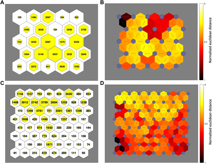
FIGURE 6. (A,C) Hits of VLP-data on the 5×5-SOM map (A), and hits of ULP-data on the 8×8-SOM map (C). Each hexagon represents one node on the map; the size of the inner yellow hexagon shows how many events fall in each node of the map. Refer to Figure 7 for the order of nodes. (B,D) The normalized euclidean distance among “nodes” prototypes of the topographic map is shown. The normalized distance between the adjacent nodes is presented with different colorings between the adjacent nodes: Dark colors (dark red) represent large distances, and light colors (light yellow) correspond to small distances among prototypes of nodes.

One standard visualization method shows the distance matrix (U-matrix), where a color scale represents prototype vector distances of adjacent nodes Figures 6B–D. The normalized euclidean distances among the corresponding prototypes are presented with different coloring between the adjacent nodes: dark/light colors between two nodes on the map indicate large/small distances between the prototypes associated with those nodes. The SOM visualizations allow an understanding of the structure of the data set: reading each node as a family of events, we can also recognize in the map the relationship between adjacent families.

In Figure 7 we visualize, on the SOM map, the histogram of when, during the year of registration, the signals falling in each node have been recorded. Notably, some nodes show a temporal distribution with very low dispersion, highly peaked in a relatively small interval of time (see for example in Figure 7 A the node 9 of VLP-SOM whose 3,222 events are quite clustered in occurrence time). Moreover, similar temporal histograms belong to adjacent nodes in the map. Since the information on the time of registration is not given to the SOM algorithm, it organizes data in the map only on the basis of shape similarity. Thus there is a correlation between time occurrence (histogram) and shape of events. Finally we visualize the normalized stacked waveform of signals for all nodes of the SOM map (Figure 8).

FIGURE 7

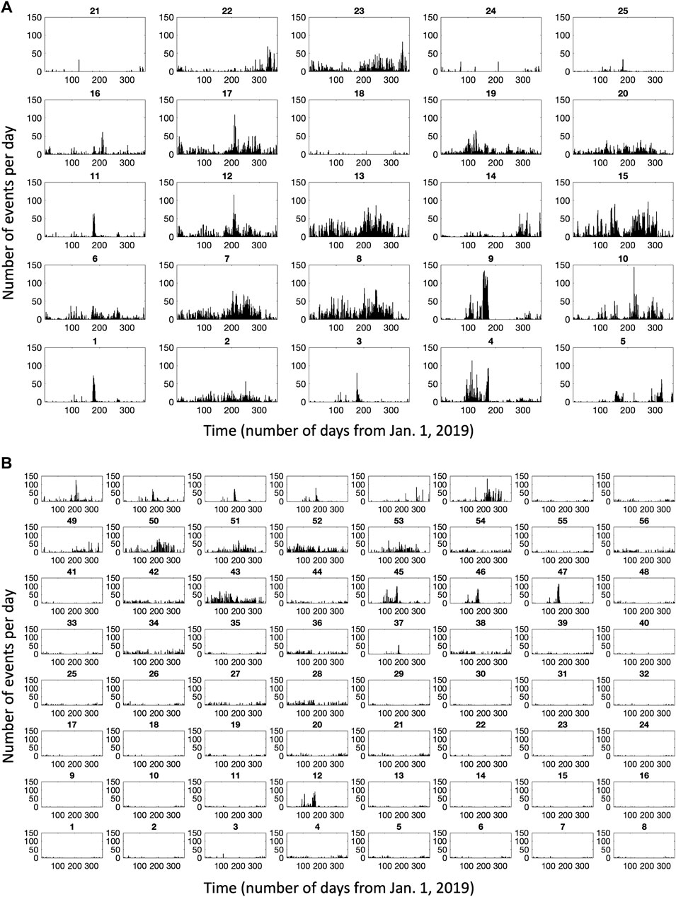
FIGURE 7. Temporal histograms of cumulative number of events per day belonging to the ith node determined by the SOM algorithm (A) events found by the VLP iteration (B) events found by the ULP iteration. The horizontal axis of the histograms indicates the time in 2019 Julian day. Signals falling in some nodes notably show a high clustering in time of occurrence. Since SOM organizes data in the map only on the basis of shape similarity, the low dispersion in the temporal distribution indicates a correlation between time occurrence (histogram) and shape of events.

FIGURE 8

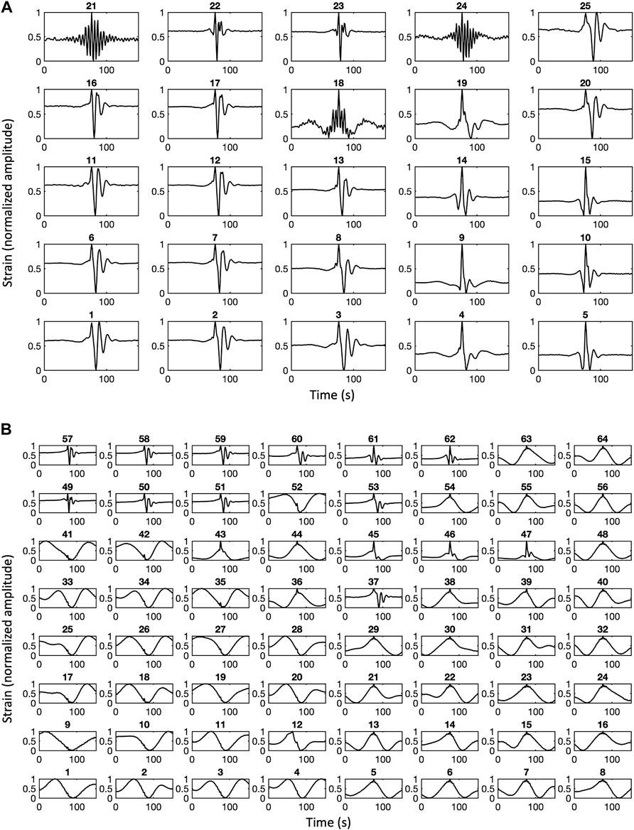
FIGURE 8. Normalized stacked waveforms belonging to the ith node of the SOM map (A) stacked waveform of families found by the VLP SOM algorithm (B) stacked waveform of families found by the ULP SOM algorithm. The horizontal axis indicates the time in seconds.

Note that the SOM algorithm, with its competitive/cooperative learning process, attempts to best visualize on the map the structure of all the N events, without discarding any data. So the 25 families of the VLP SOM cover all the VLP dataset with N=60,826 events while the 64 families of the ULP SOM cover all N =57,826 events triggered by the automated STA/LTA algorithm. Comparing Figures 5, 8, we observe that there are some stacked waveform of SOM nodes that do not have the equivalent in the stacked waveform of CC families (for example stacked waveform of node 18,19,21,22,23 24 in Figure 8A do not appear in Figure 5A). Indeed while the CC algorithm, based on a given threshold, does not arrange all the events within families, the SOM allocates all the data, trying to preserve the topology of the multi-dimensional data when they are transformed into a lower dimensional space.

3.3 Link between VLP- ULP seismicity and volcanic activity

A significant number of events belonging to several families tend to occur in specific time frames within the year 2019, as hinted by Figures 4, 7. While several events, which mainly could be associated with bad weather conditions or with a more frequent volcano dynamics, are spread across the year, some transients seem to occur prior to volcanic events. This led us to try to group them in clusters of families, to find a simultaneous occurrence. These clusters of families, determined by both methodologies as reported in Figures 9, 10, are correlated with different volcanic activity.

FIGURE 9

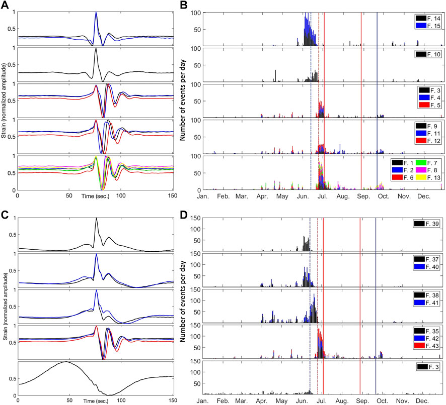
FIGURE 9. CC cluster of families correlated with different volcanic activity (A,C) VLP and ULP Normalized stacked waveforms respectively (B,D) Histograms of VLP- and ULP- data. Both spectral intervals locate families whose cumulative number of events per day tend to change as July 3 paroxysm approaches. For ULP events, a “bad weather condition” family (Family 3 in the last panel) is plotted to show its different shape in respect to volcanic activity families. The blue dashed line marks the VT occurrence on June, 13; the red dashed line marks a major explosion; the two red vertical solid lines mark the two paroxysmal events; the blue solid line marks the lowering of the explosive activity level.

FIGURE 10

FIGURE 10. SOM cluster of families correlated with different volcanic activity (A,C) VLP and ULP Normalized stacked waveforms respectively. The horizontal axis indicates the time in seconds (B,D) Histograms of VLP- and ULP- data. The horizontal axis in B of the histograms indicates the time in 2019 Julian day. Both spectral intervals locate families whose cumulative number of events per day tend to change as July 3 paroxysm approaches. SOM algorithm finds an “ordinary volcanic activity” family in VLP and ULP iteration (families 6 and 62, respectively). The blue dashed line marks the VT occurrence on June, 13; the red dashed line marks a major explosion; the two red vertical solid lines mark the two paroxysmal events; the blue solid line marks the lowering of the explosive activity level.

In case of the VLP iteration, the analysis conducted on the signals led us to the following results (Figures 9A,B and Figures 10A,B):

during June 3 we found the abrupt appearance of families 14 and 15 (from the CC analysis) or 9 (for SOM analysis), which lasts up to June 25, gradually decreasing in number of events; in the same time frame, family 10 and family 4 (from CC and SOM analysis, respectively) have the opposite behavior, gradually increasing the number of events per day. In both cases, families suddenly disappear on June 25;

after June 25, families 3, 4 and 5 (CC) and 1, 11 and 25 (SOM) slowly increase, until the paroxysm occurred on July 3, when the average number of events per day drops to a negligible level; during the same period, more families are found (1, 2, 6, 7, 8 and 13 through the CC; 3 through the SOM), showing a decreasing trend in time;

more family groups (9, 11 and 12, CC) are found in the same period; their waveforms slightly differ with respect to each other, showing a mild increase in events per day as the paroxysm approaches, while wavelengths show a faint increase;

SOM algorithm defines the steady volcanic state with one particular family, denoted 6, whose shape is very similar to families 1, 11 and 25, which is spread throughout the year, but suddenly disappears in June 25-July. Correspondent events found through the CC algorithm are distributed in more families, due to the self-similarity in shape of the transients found.

A similar analysis conducted on the signals found via the ULP iteration achieved similar conclusions, apart from the families found in the ULP iteration, both by using CC (Figure 5B) and SOM (Figure 8B) techniques, that are characterized by a lower frequency tremor present when there are bad weather conditions and/or rough sea (e.g., family 3 in Figure 9C). Considering the remaining families, they well characterize the volcano dynamics, determining similar time periods as those found by using the VLP results (Figures 9C,D and Figures 10C,D):

the CC algorithm found three groups of families (39, 37–40 and 38–41) whose appearance is limited to the period June 5-June 25. The appearance of family 39 occurs simultaneously with families 37 & 40, but, while in mid June family 39 suddenly disappears, families 37 & 40 have a gradual decrease, in contrast with families 38 & 41 whose events start to rise at the beginning of the month, dropping to low levels at the end of the period; in the same period, similarly, SOM highlights families 12, 46 and 47 which tend to decrease as the competing family 45 begins to appear;

on June 13, as a VT event is recorded, both CC and SOM algorithm found a sudden change in families shape: families 37, 39 and 40 disappear in the CC as families 38 and 41 are found; analogously, the SOM marks a clear change from family 47 to family 46;

after June 25, the previous families are not found again by either methodology, while other families suddenly appear: CC was capable of finding families 35, 42 and 43, while SOM found families 37, 57, 58 and 59. In both cases, these families dropped to almost zero events per day just after July 3;

SOM algorithm determines a particular family (62) during July - November 2019.

At the beginning of June 2019 continuous thermal anomalies recorded from MODIS data have been observed (Mattia et al., 2021). On June 13 there was a volcano-tectonic event (VT) and on June 25 a major eruption occurred (Giudicepietro et al., 2020). On July 3 the first paroxysmal eruption defined a further change in volcano dynamics, while on August 28 a second paroxysmal eruption took place. The explosive activity levels remained very high (25–35 events/hour) until waning after 20 September (Andronico et al., 2021). At the beginning of November the tremor amplitude drastically decreased [reported in the INGV surveillance bulletins (http://www.ct.ingv.it)].

Considering the volcanic activity described above, we note the appearance of a correlation between volcano phenomenology and results of our analyses.

An application of the SOM algorithm to the VLP events occurring in May 2018 - December 2020 (Figure 11) has been carried out to evaluate the performance and to test the methodology. It confirmed the results previously found. In this period, seven further major explosions (18 August 2018; July 19, August 13, November 10, 16, 21, 6 December 2020 - INGV surveillance bulletins) and hybrid events (31 March 2020) occurred. The 19 July 2020 event is an anomalous explosion, classified by Calvari et al. (2021) as a paroxysm. The SOM proved capable of finding families as well as their temporal occurrence Figures 11A,B in the period. As shown in Figures 11C,D, the specific sequence of occurrence of families found before 3 July 2019, does not happen elsewhere, while families 6 and 12 well define the post-eruptive phases of the two major explosions occurring on 18 August 2018 and 19 July 2020, respectively. It is remarkable that there is an increase in the number of events belonging to family 12 recorded after the anomalous explosion occurring in July 2020, which is followed by a gradual decrease in the upcoming days. Another peculiar period, in which all the evidenced families are found, is represented by the months January-May 2020, which is characterized by the occurrence of hybrid events.

FIGURE 11

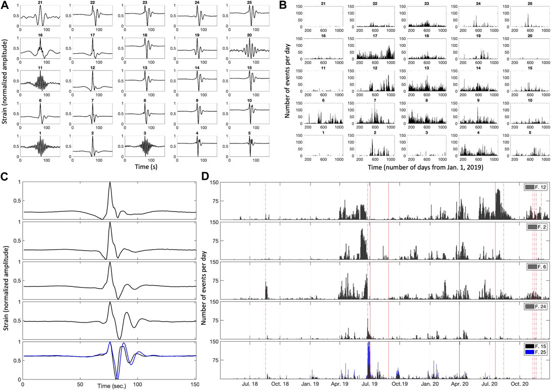
FIGURE 11. SOM cluster of families found in May 2018-December 2020 (A) Normalized stacked waveforms belonging to the ith node of the SOM map (B) Temporal histograms of cumulative number of events per day belonging to the ith node determined by the SOM algorithm (C,D) Normalized stacked waveforms and histograms of VLP data for noticeable families: black solid line marks the occurrence of the hybrid events on 31 March 2020; red dashed lines mark major explosions; the two red vertical solid lines mark the two paroxysmal events.

4 Discussion

In this work, for the first time, we statistically analyzed dilatation data content in the frequency band 2–200 s by using two independent methods to improve the robustness of the results, which led us in defining families of VLP/ULP events.

A recent classification of strain and seismic VLP waveforms in different “families” has been reported, on Mt. Stromboli, by Giudicepietro et al. (2020) and by Mattia et al. (2021). The transition from one VLP family to another, or the superposition of several seismic VLP families, has been interpreted as an indicator of changes in the fluid properties, such as the change in permeability of the higher portion of the magma in the main conduit and this can be considered an alteration of the normal condition leading to the mild ordinary explosive activity.

Due to the receiver-source distance (about 1 km) and wavelength of the analyzed signals (of the order of 10 km), we can consider the near field condition: the time history of VLP displacement reflects the source time function and can be considered to be a time dependent quasi-static volume displacement of the source (Chouet et al., 2003; Legrand et al., 2005). VLP families are related, hence, to the same source process and comparable locations, linked to fluid mass transport and the upward migration of gas slugs.

In previous articles, two basic families refer to the two main different vents and conduits. Moreover, since seismic VLPs are linked to inertial displacement of material in which they propagate (Ohminato et al., 1998; Chouet et al., 2005), the different characteristic waveform of two types suggests two origins: a variation in mechanical magma properties or a different location. In Giudicepietro et al. (2020), all seismic VLPs show little variation in incidence angle and azimuth and, starting from 25 June, become very spatially concentrated. The locations do not show remarkable variations before or during the eruptive phase of summer 2019. Mattia et al. (2021, see Figure 9) show as no direct correlation between recorded family types and vents activity is found. Furthermore, as is known from simplified models of seismo-volcanic sources (Chouet, 1986; Chouet, 1988; Chouet, 1992; Chouet and Matoza, 2013; Park et al., 2020), the resonance frequency and damping of the system is strongly influenced by the nature of liquid and gas content. These observations seem to reinforce the first hypothesis. Recent detailed analysis performed at Stromboli, with near source instruments, led Ripepe et al. (2021) to relate seismic VLP to pressurization/depressurization of the uppermost slug of magma, supporting the three-phase plug model proposed by Suckale et al. (2016). In contrast, an explanation of strain VLP shape characteristic is not available in the literature: the work by Mattia et al. (2021) is a starting point in understanding the volcanic processes on which these observations are based. The principal difference is in the time history of the source, which can be affected by the process generating the volumetric component of the source. Passage of a gas slug through the upper conduit-vent system coupled with the properties of the gas slug itself can influence the explosion nucleation and consequently the time history of the seismic source, influencing the VLP waveform. The repetitive waveform type associated with activity at a given vent suggests that usually the source process recurs in very similar conditions.

Waves radiated during the bubble growth stage may move freely through the expanding magma due to its lower damping, and under favorable conditions these waves may actually be amplified.

When the first arrival phase is tensile, the system utilizes bubble growth for additional acoustic energy and for higher wave amplitudes. On this basis we suggest a new conceptual model, in which under amplifying conditions, cycles of pressurization and depressurization of bubbly magma could be responsible for the initial amplification phase seen in LP and VLP signals.

In Kurzon et al. (2011), the analysis presented showed that when a viscous bubbly magma expands, damping is reduced (even if amplification conditions are not reached) and the medium becomes transparent, allowing unimpeded propagation of pressure waves. Legrand and Petron (2022) propose a new way of modeling and interpreting VLPs at Stromboli as the quasi-static ground-displacement field due to pressure variation of a spatially extended conduit, partially filled with magma, as a pump-like model. VLPs hence are interpreted as the elastic near- or quasi-static field ground displacement generated by a magma column under pressure. VLPs time history is characterized by a pre-eruptive expanding phase, corresponding to the increase of the pressure inside the magma column, and a post-eruptive contracting phase, corresponding to the decrease of the inner magma-column pressure. These two phases are followed by a few oscillations of the conduit/edifice. In this way, the different VLP shapes found seem to be compatible with a damped harmonic oscillator model, with changes occurring in the propagation medium properties, strengthening once again the hypothesis already made in Mattia et al., 2021.

On the basis of laboratory models, additionally, Oppenheimer et al. (2020) have proposed the important role of near-surface (down to 800 m) crystallization and the variations of the crystallinity and the interactions of crystal-bubbles in regulating the intensity of degassing and explosive activity. These authors proposed a “weak plug” model for Strombolian explosions, evolving from low viscosity style towards more crystalline, a stronger and less permeable plug corresponding to larger events. These last events are characterized by an increase in the crystallinity, determining a different conduit condition and larger size explosions. This model predicts some features of the Strombolian explosions, such as the variability of their sizes, duration, pulsation and fountaining according to the degree of near-surface crystallization, but suffers from a lack of a quantitative explanation of geophysical signals.

Petrological evidence, based on textural and chemical rock features, strengthens the weak plug model based on observations of earlier explosions, as discussed in Caracciolo et al. (2021): they suggest that dense, degassed and crystal-rich magma formed a “soft” rheological plug at the top of the conduit. Under such a condition, bubbles can accumulate under the plug to slowly build the pressure to a threshold point, after which the pressure is enough to cause the fragmentation of the plug.

Classification of strain VLP/ULP waveforms in different families and their variation over time, could be the missing piece to understand the source mechanism and to evaluate the volcanic hazard from explosive activity. The transition from one VLP family to another can be an indicator of changes in the fluid properties, such as the change in permeability of the higher portion of the magma in the main conduit and this can be considered an alteration of the normal condition leading to the mild ordinary explosive activity. In our opinion, a high rate (N > 100/day) and change in the family shape strain VLPs from “ordinary” to one “month before” (see Figure 2A) indicate a high likelihood for an impending change in volcanic activity which could lead to an explosive event within the next weeks. In this sense, this information could improve our capability to forecast dramatic events such as the one which occurred in July 2019.

5 Conclusion

In the present work, the SOM and CC algorithms have been able to discriminate little differences in VLPs shape and to find a correspondence among a higher number of families and volcanic phenomenologies. Starting from June 2019 the VLPs shape at Stromboli changes, showing a minor number of oscillations until June 25, when the shape matches the previous one. A fundamental role in these shape variations is hence played by the damping factor associated with each VLPs family found. Considering the receiver-source distance and wavelength of the analyzed signals, we are in the near field condition, which gives clues about the strain changes occurring at the source.

All the findings related with the changes in VLPs shapes lead us to propose that from June 3 until 25 June 2019, a continuous increase in the viscosity of the upper section of the magma column occurred, a hypothesis also supported by recent geophysical models, laboratory works and petrological findings. The self-organized neural system has the intrinsic capability of the SOM to analyze large sets of high dimensional data and moreover it can be implemented in an on-line learning manner. This allowed us to validate the findings that the ordered sequence of specific families brings to medium-term anomalies on a larger dataset, leading to peculiar volcano behavior.

In the present work we found that the VLP shape changes can be used as a precursor, especially for paroxysmal events occurring outside long-lasting eruptions in open-conduit volcanoes, such as Stromboli: as the VLP shape varies, suggesting an evolution in the rheological properties of the upper portion of the magma column, an impending outburst becomes more likely to occur.

The innovative analysis of dynamic strain carried out in this work, allowed us to find a medium-term (days to weeks) precursor capable of forecasting an incoming paroxysmal eruption. Considering that also short term (several minutes) strain transients are very clearly detected by the borehole strainmeters installed on Stromboli volcano, we are confident that the installation of an additional borehole instrument, which could supply information about the wavefield direction, could improve our knowledge of the mechanisms of ground deformation, linked to the pressurization processes leading to the most relevant episodes (major explosions or paroxysms) of volcanic activity.

Finally, the present work provides evidence that the dynamic strain could be useful for the knowledge of the open-conduit volcano dynamic processes and the deployment of an early warning system for eruption monitoring.

Data availability statement

The original contributions presented in the study are included in the article/Supplementary Material, further inquiries can be directed to the corresponding author.

Author contributions

PR, BD, and RS contributed to conception and design of the study. PR and BD organized the database. PR, SS, and IA performed the statistical analysis. PR and BD wrote the first draft of the manuscript. PR, BD, SS, and IA wrote sections of the manuscript. RS and AL investigated the results. All authors contributed to manuscript revision, read, and approved the submitted version.

Funding

This research was funded by the Project FIRST-ForecastIng eRuptive activity at Stromboli volcano: timing, eruptive style, size, intensity, and duration, INGV-Progetto Strategico Dipartimento Vulcani 2019 (Delibera n. 144/2020; Scientific Responsibility: S.C.). The research has moreover benefited from funding provided by the agreement between Istituto Nazionale di Geofisica e Vulcanologia (INGV) and the Italian Presidenza del Consiglio dei Ministri, Dipartimento della Protezione Civile (DPC—Presidency of the Council of Ministers—Italian Civil Protection Department).

Acknowledgments

The authors thank all the technicians and researchers involved in the hard work of maintenance and implementation of the INGV OE and INGV OV monitoring networks.

Conflict of interest

The authors declare that the research was conducted in the absence of any commercial or financial relationships that could be construed as a potential conflict of interest.

Publisher’s note

All claims expressed in this article are solely those of the authors and do not necessarily represent those of their affiliated organizations, or those of the publisher, the editors and the reviewers. Any product that may be evaluated in this article, or claim that may be made by its manufacturer, is not guaranteed or endorsed by the publisher.

Supplementary Material

The Supplementary Material for this article can be found online at: https://www.frontiersin.org/articles/10.3389/feart.2022.862086/full#supplementary-material

References

Allen, R. V. (1978). Automatic earthquake recognition and timing fromsingle traces. Bull. Seismol. Soc. Am. 68, 1521–1532. doi:10.1785/BSSA0680051521

CrossRef Full Text | Google Scholar

Andronico, D., Del Bello, E., D’Oriano, C., Landi, P., Pardini, F., Scarlato, P., et al. (2021). Uncovering the eruptive patterns of the 2019 double paroxysm eruption crisis of Stromboli volcano. Nat. Commun. 12, 4213. doi:10.1038/s41467-021-24420-1

PubMed Abstract | CrossRef Full Text | Google Scholar

Aster, R., Mah, S., Kyle, P., McIntosh, W., Dunbar, N., Johnson, J., et al. (2003). Very long period oscillations of mount erebus volcano. J. Geophys. Res. 108 (B11), 2522. doi:10.1029/2002JB002101

CrossRef Full Text | Google Scholar

Barbour, A. J., and Agnew, D. C. (2012). Detection of seismic signals using seismometers and strainmeters. Bull. Seismol. Soc. Am. 102 (6), 2484–2490. doi:10.1785/0120110298

CrossRef Full Text | Google Scholar

Bergen, K. J., Johnson, P. A., de Hoop, M. V., and Beroza, G. C. (2019). Machine learning for data-driven discovery in solid Earth geoscience. Science 363, eaau0323. eaau0323. doi:10.1126/science.aau0323

PubMed Abstract | CrossRef Full Text | Google Scholar

Bertagnini, A., Di Roberto, A., and Pompilio, M. (2011). Paroxysmal activity at Stromboli: Lessons from the past. Bull. Volcanol. 73 (9), 1229–1243. doi:10.1007/s00445-011-0470-3

CrossRef Full Text | Google Scholar

Bevilacqua, A., Bertagnini, A., Pompilio, M., Landi, P., Del Carlo, P., Di Roberto, A., et al. (2020). Major explosions and paroxysms at Stromboli (Italy): A new historical catalog and temporal models of occurrence with uncertainty quantification. Sci. Rep. 10, 17357. doi:10.1038/s41598-020-74301-8

PubMed Abstract | CrossRef Full Text | Google Scholar

Black, P. (1998). Dictionary of algorithms and data structures. Gaithersburg, MD: NISTIR. [Available at] http://www.nist.gov/dads (Accessed September 6, 2021).

Google Scholar

Bonaccorso, S., Calvari, S., Linde, A., Sacks, S., and Boschi, E. (2012). Dynamics of the shallow plumbing system investigated from borehole strainmeters and cameras during the 15 March, 2007 vulcanian paroxysm at Stromboli Volcano. Earth Planet. Sci. Lett. 357–358, 249–256. doi:10.1016/j.epsl.2012.09.009

PubMed Abstract | CrossRef Full Text | Google Scholar

Borcherdt, R. D., Johnston, M. J. S., and Glassmoyer, G. (1989). On the use of volumetric strain meters to infer additional characteristics of short-period seismic radiation. Bull. Seismol. Soc. Am. 79 (4), 1006–1023.

Google Scholar

Braun, T. (2008). On the origin of seismic signals recorded on Stromboli volcano. Würzburg: Dissertation. Available at: https://opus.bibliothek.uni-wuerzburg.de/opus4-wuerzburg/frontdoor/deliver/index/docId/2740/file/BraunThomas_Diss.pdf.

Google Scholar

Braun, T., and Ripepe, M. (1993). Interaction of seismic and air waves recorded at Stromboli Volcano. Geophys. Res. Lett. 20 (1), 65–68. doi:10.1029/92GL02543

CrossRef Full Text | Google Scholar

Buonaccorso, A. (1998). Evidence of a dyke-sheet intrusion at Stromboli volcano inferred through continuous tilt. Geophys. Res. Lett. 25 (22), 4225–4228. doi:10.1029/1998GL900115

CrossRef Full Text | Google Scholar

Calvari, S., Giudicepietro, F., Di Traglia, F., Bonaccorso, A., Macedonio, G., and Casagli, N. (2021). Variable magnitude and intensity of strombolian explosions: Focus on the eruptive processes for a first classification scheme for Stromboli volcano (Italy). Remote Sens. (Basel). 13, 944. doi:10.3390/rs13050944

CrossRef Full Text | Google Scholar

Calvari, S., Lodato, L., Steffke, A., Cristaldi, A., Harris, A. J. L., Spampinato, L., et al. (2010). The 2007 Stromboli eruption: Event chronology and effusion rates using thermal infrared data. J. Geophys. Res. 115, B04201. doi:10.1029/2009jb006478

CrossRef Full Text | Google Scholar

Calvari, S., Spampinato, L., Lodato, L., Harris, A. J. L., Patrick, M. R., Dehn, J., et al. (2005). Chronology and complex volcanic processes during the 2002–2003 flank eruption at Stromboli volcano (Italy) reconstructed from direct observations and surveys with a handheld thermal camera. J. Geophys. Res. 110, B02201. doi:10.1029/2004JB003129

CrossRef Full Text | Google Scholar

Caracciolo, A., Gurioli, L., Marianelli, P., Bernard, J., and Harris, A. (2021). Textural and chemical features of a “soft” plug emitted during strombolian explosions: A case study from Stromboli volcano. Earth Planet. Sci. Lett. 559, 116761. doi:10.1016/j.epsl.2021.116761

CrossRef Full Text | Google Scholar

Carniel, R., Barazza, F., Tárraga, M., and Ortiz, R. (2006b). On the singular values decoupling in the singular spectrum analysis of volcanic tremor at Stromboli. Nat. Hazards Earth Syst. Sci. 6, 903–909. doi:10.5194/nhess-6-903-2006

CrossRef Full Text | Google Scholar

Carniel, R., Barbui, L., and Jolly, A. (2013a). Detecting dynamical regimes by self-organizing map (SOM) analysis: An example from the March 2006 phreatic eruption at raoul island, New Zealand kermadec arc. Boll. Geofis. Teor. Appl. 54, 39–52. doi:10.4430/bgta0077

CrossRef Full Text | Google Scholar

Carniel, R. (2014). Characterization of volcanic regimes and identification of significant transitions using geophysical data: A review. Bull. Volcanol. 76, 848. doi:10.1007/s00445-014-0848-0

CrossRef Full Text | Google Scholar

Carniel, R., and Di Cecca, M. (1999). Dynamical tools for the analysis of long term evolution of volcanic tremor at Stromboli. Ann. Geofis. 42 (3), 483–495.

Google Scholar

Carniel, R., and Guzmán, S. R. (2020). Machine learning in volcanology: A review, updates in volcanology - transdisciplinary nature of volcano science. Károly Németh: IntechOpen. Available from: https://www.intechopen.com/chapters/73667. doi:10.5772/intechopen.94217

CrossRef Full Text | Google Scholar

Carniel, R., Jolly, A., and Barbui, L. (2013b). Analysis of phreatic events at Ruapehu volcano, New Zealand using a new SOM approach. J. Volcanol. Geotherm. Res. 254, 69–79. doi:10.1016/j.jvolgeores.2012.12.026

CrossRef Full Text | Google Scholar

Carniel, R., Ortiz, R., and Di Cecca, M. (2006a). Spectral and dynamical hints on the timescale of preparation of the 5 April 2003 explosion at Stromboli volcano. Can. J. Earth Sci. 43, 41–55. doi:10.1139/e05-093

CrossRef Full Text | Google Scholar

Cauchie, L., Saccorotti, G., and Bean, C. J. (2015). Amplitude and recurrence time analysis of LP activity at Mount Etna, Italy. J. Geophys. Res. Solid Earth 120, 6474–6486. doi:10.1002/2015JB011897

CrossRef Full Text | Google Scholar

Chouet, B. (1992). “A seismic model for the source of long-period events and harmonic tremor,” in IAVCEI proceedings in volcanology (Wiesbaden, Germany: Springer Gabler), 133–156.

CrossRef Full Text | Google Scholar

Chouet, B., Dawson, P., and Arciniega-Ceballos, A. (2005). Source mechanism of Vulcanian degassing at Popocatépetl Volcano, Mexico, determined from waveform inversions of very long period signals. J. Geophys. Res. 110, B07301. doi:10.1029/2004JB003524

CrossRef Full Text | Google Scholar

Chouet, B., Dawson, P., and Martini, M. (2008). “Shallow conduit dynamics at Stromboli Volcano, Italy, imaged from waveform inversion,”. Editor J. S. Gilbert (Lane: Geological Society, London, Special Publications), 307, 57–84. doi:10.1144/SP307.5Fluid Motions Volcan. Conduits A Source Seismic Acoust. Signals

CrossRef Full Text | Google Scholar

Chouet, B., Dawson, P., Ohminato, T., Martini, M., Saccorotti, G., Giudicepietro, F., et al. (2003). Source mechanisms of explosions at Stromboli Volcano, Italy, determined from moment-tensor inversions of very-long period data. J. Geophys. Res. 108 (B1), ESE 7-1–ESE 7-25. doi:10.1029/2002JB001919

CrossRef Full Text | Google Scholar

Chouet, B. (1986). Dynamics of a fluid-driven crack in three dimensions by the finite difference method. J. Geophys. Res. 91, 13967–13992. doi:10.1029/jb091ib14p13967

CrossRef Full Text | Google Scholar

Chouet, B., and Matoza, R. S. (2013). A multi-decadal view of seismic methods for de- tecting precursors of magma movement and eruption. J. Volcanol. Geotherm. Res. 252, 108–175. doi:10.1016/j.jvolgeores.2012.11.013

CrossRef Full Text | Google Scholar

Chouet, B. (1988). Resonance of a fluid-driven crack: Radiation properties and implications for the source of long-period events and harmonic tremor. J. Geophys. Res. 93, 4375–4400. doi:10.1029/jb093ib05p04375

CrossRef Full Text | Google Scholar

Chouet, B., Saccorotti, G., Dawson, P., Martini, M., Scarpa, R., De Luca, G., et al. (1999). Broadband measurements of the sources of explosions at Stromboli Volcano, Italy. Geophys. Res. Lett. 26 (13), 1937–1940. doi:10.1029/1999GL900400

CrossRef Full Text | Google Scholar

Corradino, C., Amato, E., Torrisi, F., Calvari, S., and Del Negro, C. (2021). Classifying major explosions and paroxysms at Stromboli volcano (Italy) from space. Remote Sens. (Basel). 13, 4080. doi:10.3390/rs13204080​

CrossRef Full Text | Google Scholar

De Matos, M. C., Osorio, P. L., and Johann, P. R. (2007). Unsupervised seismic facies analysis using wavelet transform and self-organizing maps. Geophysics 72 (1), 9–21. doi:10.1190/1.2392789

CrossRef Full Text | Google Scholar

Dempsey, D. E., Cronin, S. J., Mei, S., and Kempa-Liher, A. W. (2020). Automatic precursor recognition and real-time forecasting of sudden explosive volcanic eruptions at Whakaari, New Zealand. Nat. Commun. 11, 3562. doi:10.1038/s41467-020-17375-2

PubMed Abstract | CrossRef Full Text | Google Scholar

Deng, D., and Kasabov, N. (2003). On-line pattern analysis by evolving self-organizing maps. Neurocomputing 51, 87–103. doi:10.1016/s0925-2312(02)00599-4

CrossRef Full Text | Google Scholar

Di Lieto, B., Romano, P., Scarpa, R., and Linde, A. T. (2020). Strain signals before and during paroxysmal activity at Stromboli volcano, Italy. Geophys. Res. Lett. 47 (21), e2020GL088521. doi:10.1029/2020GL088521

CrossRef Full Text | Google Scholar

Di Luccio, F., Persaud, P., Cucci, L., Esposito, A., Carniel, R., Cortés, G., et al. (2021). The seismicity of lipari, aeolian islands (Italy) from one-month recording of the LIPARI array. Front. Earth Sci. 9, 678581. doi:10.3389/feart.2021.678581

CrossRef Full Text | Google Scholar

Esposito, A., Giudicepietro, F., D’Auria, L., Scarpetta, S., Martini, M., Coltelli, M., et al. (2008). Unsupervised neural analysis of very-long-period events at Stromboli volcano using the self-organizing maps. Bull. Seismol. Soc. Am. 98 (5), 2449–2459. doi:10.1785/0120070110

CrossRef Full Text | Google Scholar

Esposito, A., Giudicepietro, F., Scarpetta, S., D’Auria, L., Marinaro, M., and Martini, M. (2006). Automatic discrimination among landslide, explosion-quake, and microtremor seismic signals at Stromboli volcano using neural networks. Bull. Seismol. Soc. Am. 96 (4A), 1230–1240. doi:10.1785/0120050097

CrossRef Full Text | Google Scholar

Essenreiter, R., Karrenbach, M., and Treitel, S. (2001). Identification and classification of multiple reflections with self‐organizing maps. Geophys. Prosp. 49 (3), 341–352. doi:10.1046/j.1365-2478.2001.00261.x

CrossRef Full Text | Google Scholar

Furuya, I., and Fukudome, A. (1986). Characteristics of borehole volume strainmeter and its application to seismology. J. Phys. Earth. 34, 257–296. doi:10.4294/jpe1952.34.257

CrossRef Full Text | Google Scholar

Giordano, G., and De Astis, G. (2021). The summer 2019 basaltic Vulcanian eruptions (paroxysms) of Stromboli. Bull. Volcanol. 83, 1. doi:10.1007/s00445-020-01423-2

CrossRef Full Text | Google Scholar

Giordano, G., and De Astis, G. (2021). The summer 2019 basaltic Vulcanian eruptions (paroxysms) of Stromboli. Bull. Volcanol. 83, 1. doi:10.1007/s00445-020-01423-2

CrossRef Full Text | Google Scholar

Giudicepietro, F., López, C., Macedonio, G., Alparone, S., Bianco, F., Calvari, S., et al. (2020). Geophysical precursors of the July-August 2019 paroxysmal eruptive phase and their implications for Stromboli volcano (Italy) monitoring. Sci. Rep. 10, 10296. doi:10.1038/s41598-020-67220-1

PubMed Abstract | CrossRef Full Text | Google Scholar

Gomberg, J., and Agnew, D. (1996). The accuracy of seismic estimates of dynamic strains: An evaluation using strainmeter and seismometer data from Piñon Flat observatory, California. Bull. Seism. Soc. Am. 86 (1A), 212–220.

Google Scholar

Green, D. N., and Neuberg, J. (2006). Waveform classification of volcanic low-frequency earthquake swarms and its implication at Soufrière Hills Volcano, Montserrat. J. Volcanol. Geotherm. Res. 153, 51–63. doi:10.1016/j.jvolgeores.2005.08.003

CrossRef Full Text | Google Scholar

Inguaggiato, S., Vita, F., Cangemi, M., and Calderone, L. (2020). Changes in CO₂ soil degassing style as a possible precursor to volcanic activity: The 2019 case of Stromboli paroxysmal eruptions. Appl. Sci. (Basel). 10 (14), 4757. doi:10.3390/app10144757

CrossRef Full Text | Google Scholar

Jaquet, O., and Carniel, R. (2003). Multivariate stochastic modelling: Towards forecasts of paroxysmal phases at Stromboli. J. Volcanol. Geotherm. Res. 128, 261–271. doi:10.1016/s0377-0273(03)00259-2

CrossRef Full Text | Google Scholar

Jaquet, O., and Carniel, R. (2001). Stochastic modelling at Stromboli: a volcano with remarkable memory. J. Volcanol. Geotherm. Res. 105, 249–262. doi:10.1016/s0377-0273(00)00254-7

CrossRef Full Text | Google Scholar

Jolly, A. D., Jousset, P., Lyons, J. J., Carniel, R., Fournier, N., Fry, B., et al. (2014). Seismo-acoustic evidence for an avalanche driven phreatic eruption through a beheaded hydrothermal system: An example from the 2012 Tongariro eruption. J. Volcanol. Geotherm. Res. 286, 331–347. ISSN 0377-0273. doi:10.1016/j.jvolgeores.2014.04.007

CrossRef Full Text | Google Scholar

Julian, B. R., Miller, A. D., and Foulger, G. R. (1997). Non-double-couple earthquake mechanisms at the Hengill-Grensdalur volcanic complex, Southwest Iceland. Geophys. Res. Lett. 24, 743–746. doi:10.1029/97GL00499

CrossRef Full Text | Google Scholar

Kirchdörfer, M. (1999). Analysis and quasistatic FE modeling of long period impulsive events associated with explosions at Stromboli Volcano (Italy). Ann. Geofis. 42, 379–390. http://hdl.handle.net/2122/1350.

Google Scholar

Kohonen, T. (2008). “Data management by self-organizing maps,” in Computational intelligence: Research Frontiers. WCCI 2008. Lecture notes in computer science. Editors J. M. Zurada, G. G. Yen, and J. Wang (Berlin, Heidelberg: Springer), Vol. 5050. doi:10.1007/978-3-540-68860-0_15

CrossRef Full Text | Google Scholar

Kohonen, T., Kaski, S., Lagus, K., Salojarvi, J., Honkela, J., Paatero, V., et al. (2000). Self organization of a massive document collection. IEEE Trans. neural Netw. 11 (3), 574–585.

PubMed Abstract | CrossRef Full Text | Google Scholar

Kohonen, T., Oja, E., Simula, O., Visa, A., and Kangas, J. (1996). Engineering applications of the self-organizing map. Proc. IEEE 84 (10), 1358–1384. doi:10.1109/5.537105

CrossRef Full Text | Google Scholar

Kohonen, T. (2001). Self-organizing maps. 3rd ed. Berlin: Springer-Verlag. first ed.: 1995.

Google Scholar

Kumagai, H., Ohminato, T., Nakano, M., Ooi, M., Kubo, A., Inoue, H., et al. (2001). Very-long-period seismic signals and caldera formation at miyake island, Japan. Science 293 (5530), 687–690. doi:10.1126/science.1062136

PubMed Abstract | CrossRef Full Text | Google Scholar

Kurzon, I., Lyakhovsky, V., Navon, O., and Chouet, B. (2011). Pressure waves in a supersaturated bubbly magma. Geophys. J. Int. 187, 421–438. doi:10.1111/j.1365-246X.2011.05152.x

CrossRef Full Text | Google Scholar

La Spina, G., PolacciBurton, M., de’ Michieli Vitturi, M. M., and de' Michieli Vitturi, M. (2017). Numerical investigation of permeability models for low viscosity magmas: Application to the 2007 Stromboli effusive eruption. Earth Planet. Sci. Lett. 473, 279–290. doi:10.1016/j.epsl.2017.06.013

CrossRef Full Text | Google Scholar

Lagus, K., Kaski, S., and Kohonen, T. (2004). Mining massive document collections by the WEBSOM method. Inf. Sci. (N. Y). 163, 135–156. doi:10.1016/j.ins.2003.03.017

CrossRef Full Text | Google Scholar

Legrand, D., and Perton, M. (2022). What are VLP signals at Stromboli volcano? J. Volcanol. Geotherm. Res. 421, 107438. doi:10.1016/j.jvolgeores.2021.107438

CrossRef Full Text | Google Scholar

Legrand, D., Rouland, D., Frogneux, M., Carniel, R., Charley, D., Roult, G., et al. (2005). Interpretation of very long period tremors at Ambrym volcano, Vanuatu, as quasi static displacement field related to two distinct magmatic sources. Geophys. Res. Lett. 32, L06314. doi:10.1029/2004GL021968

CrossRef Full Text | Google Scholar

Martini, M., Giudicepietro, F., D’Auria, L., Esposito, A. M., Caputo, T., Curciotti, R., et al. (2007). Seismological monitoring of the February 2007 effusive eruption of the Stromboli volcano. Ann. Geophys. 50, 775–788. doi:10.4401/ag-3056

CrossRef Full Text | Google Scholar

Mattia, M., Aloisi, M., Di Grazia, G., Gambino, S., Palano, M., and Bruno, V. (2008). Geophysical investigations of the plumbing system of Stromboli volcano (Aeolian Islands, Italy). J. Volcanol. Geotherm. Res. 176 (4), 529–540. doi:10.1016/j.jvolgeores.2008.04.022

CrossRef Full Text | Google Scholar

Mattia, M., Di Lieto, B., Ganci, G., Bruno, V., Romano, P., Ciancitto, F., et al. (2021). The 2019 eruptive activity at Stromboli volcano: A multidisciplinary approach to reveal hidden features of the “unexpected” 3 july paroxysm. Remote Sens. (Basel). 13, 4064. doi:10.3390/rs13204064

CrossRef Full Text | Google Scholar

McGreger, A. D., and Lees, J. M. (2004). Vent discrimination at strombolivolcano, Italy. J. Volcanol. Geotherm. Res. 137, 169–185. doi:10.1016/j.jvolgeores.2004.05.007

CrossRef Full Text | Google Scholar

Métrich, N., Bertagnini, A., and Pistolesi, M. (2021). Paroxysms at Stromboli volcano (Italy): Source, Genesis and dynamics. Front. Earth Sci. 9, 593339. doi:10.3389/feart.2021.593339

CrossRef Full Text | Google Scholar

Miller, A., Stewart, R. L., White, R. A., Luckett, R., Baptie, B. J., Aspinall, W. P., et al. (1998). Seismicity associated with dome growth and collapse at the Soufrière Hills Volcano, Montserrat. Geophys. Res. Lett. 25 (18), 3401–3404. doi:10.1029/98gl01778

CrossRef Full Text | Google Scholar

Musil, M., and Plešinger, A. (1996). Discrimination between local microearthquakes and quarry blasts by multi-layer perceptrons and Kohonen maps. Bull. Seism. Soc. Am. 86 (4), 1077–1090.

Google Scholar

Naim, A., Ratnatunga, K. U., and Griffiths, R. E. (1997). Galaxy morphology without classification: Self-organizing maps. Astrophys. J. Suppl. Ser. 111, 357–367. doi:10.1086/313022

CrossRef Full Text | Google Scholar

Neuberg, J., Luckett, R., Ripepe, M., and Braun, T. (1994). Highlights from a seismic broadband array on Stromboli Volcano. Geophys. Res. Lett. 21 (9), 749–752. doi:10.1029/94GL00377

CrossRef Full Text | Google Scholar

Nishimura, T., Nakamichi, H., Tanaka, S., Sato, M., Kobayashi, T., Ueki, S., et al. (2000). Source process of very long period seismic events associated with the 1998 activity of Iwate Volcano, northeastern Japan. J. Geophys. Res. 105 (B8), 19135–19147. doi:10.1029/2000JB900155

CrossRef Full Text | Google Scholar

Ohminato, T., Chouet, B., Dawson, P., and Kedar, S. (1998). Waveform inversion of very long period impulsive signals associated with magmatic injection beneath Kilauea volcano, Hawaii. J. Geophys. Res. 103, 23839–23862. doi:10.1029/98JB01122

CrossRef Full Text | Google Scholar

Oppenheimer, J., Capponi, A., Cashman, K., Lane, S., Rust, A., and James, M. (2020). Analogue experiments on the rise of large bubbles through a solids-rich suspension: A “weak plug” model for strombolian eruptions. Earth Planet. Sci. Lett. 531, 115931. doi:10.1016/j.epsl.2019.115931

CrossRef Full Text | Google Scholar

Park, I., Jolly, A., Lokmer, I., and Fennedy, B. (2020). Classification of long-term very long period (VLP) volcanic earthquakes at Whakaari/White Island volcano, New Zealand. Earth Planets Space 72, 92. doi:10.1186/s40623-020-01224-z

CrossRef Full Text | Google Scholar

Pino, N. A., Moretti, R., Allard, P., and Boschi, E. (2011). Seismic precursors of a basaltic paroxysmal explosion track deep gas accumulation and slug upraise. J. Geophys. Res. 116, B02312. doi:10.1029/2009JB000826

CrossRef Full Text | Google Scholar

Ripepe, M., Delle Donne, D., Legrand, D., Valade, S., and Lacanna, G. (2021). Magma pressure discharge induces very long period seismicity. Sci. Rep. 11, 20065. doi:10.1038/s41598-021-99513-4

PubMed Abstract | CrossRef Full Text | Google Scholar

Ripepe, M., Marchetti, E., Delle Donne, D., Genco, R., Innocenti, L., Lacanna, G., et al. (2018). Infrasonic early warning system for explosive eruptions. J. Geophys. Res. Solid Earth 123 (11), 9570–9585. doi:10.1029/2018JB015561

CrossRef Full Text | Google Scholar

Ripepe, M., Rossi, M., and Saccorotti, G. (1993). Image processing of explosive activity at Stromboli. J. Volcanol. Geotherm. Res. 54, 335–351. doi:10.1016/0377-0273(93)90071-X

CrossRef Full Text | Google Scholar

Seydoux, L., Balestriero, R., Poli, P., de Hoop, M., Campillo, M., and Baraniuk, R. (2020). Clustering earthquake signals and background noises in continuous seismic data with unsupervised deep learning. Nat. Commun. 11, 3972. doi:10.1038/s41467-020-17841-x

PubMed Abstract | CrossRef Full Text | Google Scholar

Silver, P. G., Bock, Y., Agnew, D., Henyey, T., Linde, A. T., McEvilly, T. V., et al. (1999). A plate boundary observatory. IRIS Newsl. 16, 3–9.

Google Scholar

Spampinato, S., Langer, H., Messina, A., and Falsaperla, S. (2019). Short-term detection of volcanic unrest at Mt. Etna by means of a multi-station warning system. Sci. Rep. 9 (1), 6506. doi:10.1038/s41598-019-42930-3

PubMed Abstract | CrossRef Full Text | Google Scholar

Suckale, J., Keller, T., Cashman, K. V., and Persson, P.-O. (2016). Flow-to-fracture transition in a volcanic mush plug may govern normal eruptions at Stromboli. Geophys. Res. Lett. 43 (23), 12071–12081. doi:10.1002/2016GL071501

CrossRef Full Text | Google Scholar

Telesca, L., Lovallo, M., and Carniel, R. (2010). Time-dependent Fisher information measure of volcanic tremor before the 5 April 2003 paroxysm at Stromboli volcano, Italy. J. Volcanol. Geotherm. Res. 1951, 78–82. doi:10.1016/j.jvolgeores.2010.06.010

CrossRef Full Text | Google Scholar

A. Vellido, K. Gibert, C. Angulo, and J. D. Martín Guerrero (Editors) (2020). “Advances in self-organizing maps, learning vector quantization, clustering and data visualization,” Advances in intelligent systems and computing 976 (Springer).

Google Scholar

Viccaro, M., Cannata, A., Cannavò, F., De Rosa, R., Giuffrida, M., Nicotra, E., et al. (2021). Shallow conduit dynamics fuel the unexpected paroxysms of Stromboli volcano during the summer 2019. Sci. Rep. 11, 266. doi:10.1038/s41598-020-79558-7

PubMed Abstract | CrossRef Full Text | Google Scholar