Enhanced Multi-Dimensional Inversion Through Target-Specific Inversion Parameter Bounds With an Application to Crosswell Electromagnetic for Sequestration Monitoring

In geophysical inversions, lower and upper model parameter bounds are a means of solution stabilization. Further, constraints that intend to let only geologically plausible inverse solutions pass are amenable to lower and upper bounds. Reliable prior information is paramount to construct such bound constraints. It is common practice to narrow and widen bound intervals for regions of, respectively, more and less certain prior information. Contrary to this practice, we experiment with widened bound intervals in zones that are poorly resolved by a given survey configuration but where prior information would suggest structural anomalies of interest. The purpose of enlarged parameter bounds that correlate spatially with predefined targets is to let the inversion explore a larger solution space, thus increasing the potential to resolve otherwise hidden anomalies. Application of the method is based on a carbon-sequestration baseline (pre-injection) crosswell electromagnetic (EM) field survey at the Containment and Monitoring Institute Field Research Station (Alberta, Canada), where impeded measurements led to generally reduced sensitivities for the interwell region. Synthetic-data proofs of concept use augmented bounds designed to boost the resolution of artificial plume targets, indicating an enhanced illumination compared to constant bounds. Comparative field data inversions with spatially variable bounds constructed from prior resistivity and velocity information highlight non-horizontal baseline structures.

1 Introduction

Geophysical inverse-modeling problems are usually hampered by data sparsity and data noise. At the same time, realistic earth models require a high degree of model discretization. The coincidence of these issues leads to a non-unique and thus ill-posed nature of solutions of pixel-based (many-parameter) inverse problems (e.g., Haber et al., 2010). A standard technique for addressing non-uniqueness is to regularize the solution-finding process through constraints that are imposed on the mathematical representation of the inverse solution (e.g., Jackson, 1979). The constrained inverse solution is commonly described as the minimization of a multi-component objective function, for example

$\theta \mathbf{(}\mathbf{m}\mathbf{)}={\theta }_d\mathbf{(}\mathbf{m}\mathbf{)}+\lambda {\theta }_{\mathit{m}}\mathbf{(}\mathbf{m}\mathbf{)}(1)$

consisting of a data component ${\theta }_d\left(\mathbf{m}\right)$ and model-regularizing component ${\theta }_m\left(\mathbf{m}\right)$, where the influence of the latter is balanced by the regularization factor $\lambda$. The data part quantifies the difference between a discrete set of noisy observations and a corresponding set of predicted responses, typically in a least-squares sense.

In our experiments, ${\theta }_d\left(\mathbf{m}\right)$ involves the fitting of electromagnetic (EM) data from a crosswell configuration (e.g., Alumbaugh and Morrison, 1995). In EM inversions, the underlying model parameter vector $\mathbf{m}$ (of size M) to be estimated describes the spatial distribution of electrical rock properties. In our case, the property of interest is electrical conductivity, to be abbreviated by $\sigma$ with unit S/m (Siemens per meter), where we use its inverse, electrical resistivity $\rho =\frac{1}{\sigma }$ with unit $\text{Ω}\text{m}$ (Ohm meter), interchangeably.

The literature on geophysical inversion usually motivates the introduction of constraints as a means to address non-uniqueness through allowing geological models that are perceived as plausible (Habashy and Abubakar, 2004; Abubakar et al., 2009; Sosa et al., 2013; Ogarko et al., 2021). Constraining the solution arising from the minimization of Eq. 1 is realized by the model-regularizing term ${\theta }_m\left(\mathbf{m}\right)$, which operates on $\mathbf{m}$, a common form being (e.g., Menke, 2018)

${\theta }_{\mathit{m}}\mathbf{(}\mathbf{m}\mathbf{)}=\lambda {\left[\mathbf{W}\left(\mathbf{m}-{\mathbf{m}}^{ref}\right)\right]}^T\mathbf{W}\left(\mathbf{m}-{\mathbf{m}}^{ref}\right)(2)$

Minimizing the total error term $\theta \left(\mathbf{m}\right)$ then essentially enforces a model solution $\mathbf{m}-{\mathbf{m}}^{ref}\mathit{ }$ to vary smoothly across contiguous elements of $\mathbf{m}$, realized through an appropriate smoothing matrix $\mathbf{W}$ (e.g., de Groot-Hedlin and Constable, 2004). Equation 2 realizes a class of constraints that can be applied collectively, by enforcing smoothness, and individually, by enforcing the proximity of all or a subset of parameters to a given reference ${\mathbf{m}}^{ref}$ (Medeiros and Silva, 1996; Farquharson et al., 2008).

It has been argued that the inversion against a fixed reference model ${\mathbf{m}}^{ref}$ can be too restrictive, because it hampers the incorporation of uncertainties associated with prior geological information (Kim et al., 1999). Further, the drawback of smoothness constraints is the suppression of actually existing strong property contrasts. While this can be addressed by setting pre-selected elements of $\mathbf{W}$ to zero (de Groot-Hedlin and Constable, 2004), it may require relatively detailed structural prior information. Another issue is that balancing the influence of ${\theta }_d\left(\mathbf{m}\right)$ and ${\theta }_m\left(\mathbf{m}\right)$ on the solution process may require a multitude of trial inversions with different regularization factors, $\lambda$ (Eq. 2) (Sosa et al., 2013). Reaching this balance still may not rule out a locally suppressed search space. A method addressing this issue, referred to as active constraint balancing, makes the regularization factor $\lambda$ spatially variable (Yi et al., 2003). Principally, the approach seeks to enhance spatial model resolution through assigning small $\lambda$-values (less constraining) in zones of high resolution. At the same time, large $\lambda$-values intend to avoid parameter overshoots in zones of low resolution. The inverse problem’s parameter resolution matrix guides the quantification of resolution.

The inversion experiments in this study pick up the concept of constraint balancing; however, we revert to the usage of bound constraints for their facilitation of prior-model fusion (Kim et al., 1999; Abubakar et al., 2008; Kim and Kim, 2011; Aghamiry et al., 2019; Ogarko et al., 2021). A priori knowledge with varying degrees of certainty lends itself to defining individual bounds a and b imposed on the model parameters $m_i$, expressed as the inequality $a_i<m_i<b_i \left(i=1,\dots ,M\right)$. Sosa et al. (2013) argued that such bound constraints allow solutions to become “more physical” than smooth models. However, there may also occur a limitation “of the space to be explored by inversion before convergence” (Ogarko et al., 2021), causing deterministic inversions to have a potentially larger tendency towards ending prematurely in local minima. Addressing this issue, lower and upper bound constraints in conjunction with the alternating direction method of multipliers have enhanced full-waveform imaging (Aghamiry et al., 2019) and gravity inversion (Ogarko et al., 2021). The multipliers essentially widen bound intervals, thus extending the inversion’s model search space during early iterations, encouraging the inversion to explore the model space outside of preset bounds. Later iterations put more weight on honoring stricter bounds.

This contribution investigates a potential model resolution enhancement enabled through spatially variable bound constraints. Our approach is a simplification of the concepts by Yi et al. (2003) and Ogarko et al. (2021) because 1) we do not employ the parameter resolution matrix for bound construction, and 2) augmented bound intervals, that is, bounds that are enlarged with respect to a default, remain static throughout the inversion. The principal idea is to allow the inversion to venture out into an enlarged model space during all model-updating iterations. Regions of enlarged bounds reflect preconceived focus zones that are suggested by prior information. Hence, we also regard this method as a simple way of conveying prior model information about anomalous zones of interest to the inversion process. Synthetic and field data demonstrations are based on a crosswell EM baseline survey conducted within a geologic carbon sequestration (GCS) context.

2 Methodology

The inverse-modeling studies of this work seek for a constrained solution using a non-linear conjugate-gradient (NLCG) scheme (e.g., Luenberger, 1984). Our NLCG implementation encompasses a three-dimensional (3D) finite-difference (FD) scheme for the forward modeling of CSEM data (Commer and Newman, 2008). The NLCG scheme minimizes an objective function of the form of Eq. 1 by performing a sequence of line-searches in model space, generating a sequence of model updates ${\mathbf{m}}_0,{\mathbf{m}}_1,\dots ,{\mathbf{m}}_{Nmax}$. The scheme has the goal of reaching a desired minimum $\theta \left({\mathbf{m}}_{N_{max}}\right)$ within some preset maximal number ($N_{max}$) of inversion iterations. Each model-updating step involves the calculation of first-derivative information of the error functional’s components in the form of gradient vectors, $\nabla \theta =\nabla {\theta }_d\left(\mathbf{m}\right)+\lambda \nabla {\theta }_m\left(\mathbf{m}\right)$. For further mathematical details, we also refer to earlier applications of NLCG to EM data inversion (e.g., Mackie and Madden, 1993; Newman and Alumbaugh, 2000). Note that our inversions operate on a representation of the complex EM fields as real and imaginary field components while we will present data fits below as pairs of amplitude and phase.

2.1 Spatially Variable Lower and Upper Parameter Bounds

Lower and upper parameter bounds $\left[a,b\right]$ constrain the evolution of a model parameter m during an inversion process, so that m is bounded by $a<m<b$. In order to impose a positivity constraint on electrical resistivity (or conductivity), the bounds usually occur in conjunction with logarithmic or hyperbolic types of parameter transformation functions. Generalized functions were formulated by Kim and Kim (2011),

$x=\frac{1}{n}\text{log}\left(\frac{m-a}{b-m}\right)=\frac{2}{n}\text{tan}{\text{h}}^{-1}\left(\frac{2m-b-a}{b-a}\right);a<m<b,(3)$

where x is the transformed parameter and n is a positive integer constant. Our studies employ a version realized by $n=1$. Transforming x back into the original model parameter space then leads to (Commer and Newman, 2008)

$m=\frac{a+b\text{e}\text{x}\text{p}\left(x\right)}{1+\text{e}\text{x}\text{p}\left(x\right)};-\infty <x<\infty .(4)$

Constant bounds may be most suitable for inversion applications where prior information is absent, that is, the bound interval $\left[a,b\right]$ applies to every cell parameter $m_i$ ($i=1,\dots ,M$) of the inversion domain. In the presence of location-dependent prior information, a and b can become spatially variable so that each cell $m_i$ is subjected to an individual bounding interval $\left[a_i,b_i\right]$.

2.2 Constructing Parameter Bounds From a Reference Model

We do not employ a priori model information, ${\mathbf{m}}^{ref}$, in a manner as given by Eq. 2. Instead, ${\mathbf{m}}^{ref}$ forms the basis for the definition of anomaly thresholds during a pre-processing step. Properties of reference cells $m_i^{ref}$ that surpass these thresholds undergo a modification of a given default bound interval, $\left[a^{def},b^{def}\right]\to \left[a^{def}-\text{Δ}a,b^{def}+\text{Δ}b\right]$. Widening the bounds by $\text{Δ}a$ and $\text{Δ}b$ for certain model zones translates to a locally widened model search space, thus heightening spatial model fidelity. The scheme resembles the concept of active constraint balancing (Yi et al., 2003); however, augmented bounds remain static throughout the whole inversion process. The bound input thus accompanies the starting-model input so that an individual bounding interval $\left[a_i,b_i\right]$ is assigned to each cell parameter $m_i$ of the starting model. Once assigned, the bound parameters $\left(a_i,b_i\right)$ remain constant, whether they define locally augmented bounds, $\left[a_i,b_i\right]=\left[a^{def}-\text{Δ}a,b^{def}+\text{Δ}b\right]$, or not, $\left[a_i,b_i\right]=\left[a^{def},b^{def}\right]$. The bound construction is thus a pre-processing step before inversion and a means of defining focus zones that are suggested by the reference ${\mathbf{m}}^{ref}$.

Our inversion operates on $\sigma$ so all following bound parameters are in units of S/m. Bound construction relies on arbitrarily chosen thresholds that qualify a given reference cell parameter $m_i^{ref}={\sigma }_i=\sigma$ as anomalous. First, we consider the case where the objective is to enhance the model resolution due to indicators for conductive anomalies, $\sigma >{\sigma }^{min}$. Here, the superscript min refers to the minimum $\sigma$ in order to qualify a cell parameter as anomalously conductive. The corresponding augmented bound interval $\left[a,b\right]$ is

$\text{log}\left(a\right)=\log \left(a^{def}\right)-m^a\left[\text{log}\left(\sigma \right)-\text{log}\left({\sigma }^{min}\right)\right], m^a=\frac{\text{log}\left(a^{def}\right)-\text{log}\left(a^{min}\right)}{\text{log}\left({\sigma }^{max}\right)-\text{log}\left({\sigma }^{min}\right)},(5)$

$\text{log}\left(b\right)=\log \left(b^{def}\right)+m^b\left[\text{log}\left(\sigma \right)-\text{log}\left({\sigma }^{min}\right)\right],m^b=\frac{\text{log}\left(b^{max}\right)-\text{log}\left(b^{def}\right)}{\text{log}\left({\sigma }^{max}\right)-\text{log}\left({\sigma }^{min}\right)}.(6)$

Keep in mind that ${\sigma }_i=\sigma$ refers to model cells of the constant reference ${\mathbf{m}}^{ref}$. Logarithmic parameters account for the typically large conductivity range of earth materials. Equations 5, 6 modify the default bounds in a linear fashion for all zones fulfilling ${\sigma }^{min}<\sigma <{\sigma }^{max}$. Outside of this range, for cells $\sigma \le {\sigma }^{min}$ one has $[a,b]=$ $\left[a^{def},b^{def}\right]$ while a predefined maximum bound interval $\left[a^{min},b^{max}\right]$ holds for all cells $\sigma \ge {\sigma }^{max}$.

For the case where the objective is to enhance the resolution in regions that exhibit resistive features in ${\mathbf{m}}^{ref}$, bounds are augmented for all cells $\sigma <{\sigma }^{max}$,

$\text{log}\left(a\right)=\log \left(a^{def}\right)-m^a\left[\text{log}\left({\sigma }^{max}\right)-\text{log}\left(\sigma \right)\right],(7)$

$\text{log}\left(b\right)=\log \left(b^{def}\right)+m^b\left[\text{log}\left(\sigma \right)-\text{log}\left({\sigma }^{min}\right)\right],(8)$

where $m^a$ and $m^b$ are as defined by Eqs 5, 6. Here, the superscript max refers to the maximum $\sigma$ in order to qualify a cell parameter as anomalously resistive (having low $\sigma$). Therefore, for cells above this threshold, $\sigma \ge {\sigma }^{max}$, $\left[a,b\right]=\left[a^{def},b^{def}\right]$ while all cells $\sigma \le {\sigma }^{min}$ are kept at the fixed maximum bound interval $\left[a^{min},b^{max}\right]$.

For the following demonstrations, it is important to keep in mind that only the (resistive or conductive) nature of outstanding features in ${\mathbf{m}}^{ref}$ will define our focus zone. For this zone, Eqs 5, 6 as well as Eqs 7, 8 enlarge bounds in both directions; hence, the widened bound intervals let both resistive and conductive parameter anomalies pass in the imaging outcome.

3 Results

The following section provides a synthetic-data and field-data proof-of-concept for the resolution-enhacing effect of spatially variable parameter bounds. The inverse modeling of crosswell EM data is based on surveys conducted at the Containment and Monitoring Institute Field Research Station (CaMI.FRS), located in Alberta, Canada. CaMI.FRS is a small-scale GCS test site for the investigation of monitoring techniques at shallow and intermediate injection depths (Um et al., 2020). An injector well and two observation wells are completed to a depth of 350 m (Figure 1A). Small volumes of CO₂ will be injected into the basal Belly River Sandstone at depths up to 300 m. The basal Belly River sandstone ranges from 17 to 21 m thick and consists of fine- to medium-grained well to very-well sorted lithic arenite (sandstone with grain sizes 0.06–2 mm and over 50% rock fragments) (Iwuagwu and Lerbekmo, 1982).

FIGURE 1

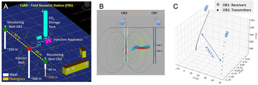
FIGURE 1. (A): Schematic view of CaMI.FRS site with injector and monitoring wells. (B): Schematic of a crosswell EM configuration. Primary EM fields are emitted in the transmitter well and recorded together with induced secondary vertical magnetic fields in an adjacent receiver well. Data processing steps separate the signals so that the rock electrical resistivity information is derived from the secondary fields. (C): Actual positions of the magnetic transmitter and receiver coils. The two wells OB1 and OB2 are deviated, with an average of 54.5 m separating the instrumented sections.

3.1 Prior Information at the CaMI Field Research Station

We first give a brief overview of the geophysical surveys conducted at CaMI.FRS. Both EM and seismic crosswell data were taken in order to characterize the pre-injection state. Our synthetic-data proof-of-concept replicates the EM survey geometry. The subsequent field-data proof-of-concept employs prior information in form of seismic images together with resistivity and velocity logs for the design of variable parameter bounds. Therefore, all prior information is introduced first.

3.1.1 Electromagnetic Crosswell Survey

Crosswell EM uses the principles of EM induction to interrogate the electrical resistivity between wells. As sketched in Figure 1B, a vertical magnetic dipole (VMD) induction coil placed in the transmitter well broadcasts sinusoidal EM signals into the formation. At the receiver well, the signals are detected, in our case via a double-coil receiver with two connected sensors separated by 5 m. Source and receiver usually traverse the wells with recordings triggered at regularly spaced intervals leading to a tomographic illumination of the interwell space.

Tomographic baseline crosswell EM data were collected over the depth section 200–320 m (Figure 1C) with a transmitter spacing of 2 m in observation borehole 2 (named OB2), thus leading to 59 source depth levels. The two-receiver string traversed 10 levels at intervals of 10 m in observation borehole 1 (OB1). Unfortunately, cross checks between signal amplitudes and receiver depth recordings revealed inconsistencies which rendered only 8 receiver sets per transmitter activation usable. While the cause remains unclear, we speculate that the bottom receiver of the double-sensor array might have buoyantly floated upwards, thus not keeping the constant reference separation (5 m) between the two sensors. Moreover, while the transmitter system operated at the two frequencies of 200 and 450 Hz, data noise turned out excessive at 450 Hz. Both issues reduced the usable data to a total of 454 complex magnetic-field data points which are the input to our field-data inversions presented below.

In addition to the data sparsity, another complication is caused by horizontal well deviations of the instrumented sections which max out at 7 m (OB2) and 0.5 m (OB1). Ensuing instrument rotations out of the horizontal plane are often neglected in academic crosswell EM studies. Given the dominating deviation of OB2, we incorporate source coil rotations in form of tilt and azimuth angles in the field-data inversions.

3.1.2 Correction for Electromagnetic Steel-Casing Effects

Croswell EM can be stymied by the signal-shielding nature of metal borehole casings, because large magnetic fields result from the transmitter coupling with hysteretic magnetic permeabilities of steel. If open holes (no casing present) cannot be realized, fiberglass casing avoids this coupling. At CaMI.FRS, the transmitter well (OB2) is steel-cased from the surface to 60 m and fiberglass-cased from 60 to 350 m, while OB1 is all steel-cased down to 350 m. The effects at frequencies below a few hundred Hz remain moderate for the received signals. Nevertheless, in the presence of weak geological effects on the data one wants to avoid any potentially overpowering casing effect. The casing effect at the receivers can be corrected for either in the course of data inversion, or it can be removed prior to the inversion process. Here we choose the latter in order to avoid the computationally demanding forward-modeling of casing effects during the inversion. The correction procedure essentially utilizes the fact that in the frequency domain one can approximate the casing effect by means of a source-signature correction with a complex factor (Wu and Habashy, 1994).

We outline the steps that correct for EM induction effects contained in receiver coils that are surrounded by steel casing. The main component is an appropriate reference model from which one can calculate non-casing reference data. The two resistivity logs in the two observation wells (Figure 2A) were employed to construct a 1D reference model. It involved fewer parameters than given by our 1D inversion presented below while being equivalent in terms of data fit. The predominantly horizontally layered geology at CaMI.FRS helps limit the error due to the approximate nature of the reference model.

FIGURE 2

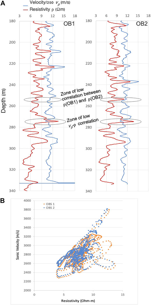
FIGURE 2. (A): Prior EM and seismic information at CaMI.FRS. Seismic-velocity ($v_p$) logs (blue, scaled by a factor of 250) and resistivity ($\rho$) logs (red) were measured in wells OB1 and OB2. Zones of low correlation are annotated only for depth sections that we consider as sufficiently resolved by the crosswell system. (B): The cross plot between velocity and resistivity measurements highlights a relatively strong degree of correlation which is minimal in a narrow depth section between 270 m and 280 m.

For each common-receiver gather of the tomographic crosswell EM data, we extract the data pertaining to all transmitter depths that are in vertical proximity, here within 5 m of the depth of the receiver gather. These data are complex magnetic-field values containing the casing effect. Replicating their survey geometry with respect to the receiver depth, we calculate a corresponding non-casing data set through forward-modeling of the 1D reference model.

For each transmitter depth of a given receiver gather, we divide the non-casing reference data by its measured counterpart. This yields a set of estimated casing-correction factors which are also complex numbers. All correction factors of one receiver gather are averaged. The outcome is a best estimate for the magnetic-field attenuation and phase shift caused by the steel casing. The averaging is carried out for all individual receiver gathers, producing a set of location-dependent best-estimate correction factors. Making the correction depth-dependent intends to limit the impact on non-casing signal footprints one wants to retain as they contain for example effects due to local 3D structures.

The final step is the actual data correction. Each data point of a given receiver gather is multiplied by the gather’s correction factor, producing a common-receiver gather of corrected data. Applying the correction procedure to each receiver gather yields a tomographic data set of casing-corrected data that are also normalized for unit source moment. This set is the data input for the field-data inversions presented here. Image distortions due to this correction procedure are limited to the vicinity around the casing (Gao et al., 2008).

3.1.3 Seismic Well Logs and Crosswell Survey

Compressional-wave velocity ($v_p$) logs were acquired in OB1 and OB2 (Figure 2A). Cross-plotting the well measurements of velocity against resistivity (Figure 2B) highlights a degree of correlation that we deem as sufficient for using $v_p$ as reference for our EM inversions. In addition to the well logs, a high-resolution crosswell seismic survey with piezoelectric seismic sources was part of the baseline data collection at CaMI.FRS (Um et al., 2020). To achieve tomographic imaging, a total of 257 total source positions traversed the well from 216 to 344 m at depth intervals of 0.5 m. Figure 3A sketches the set of ray paths resulting from one source activation. Seismic signals were recorded in well OB2 using a string of broadband hydrophone receivers. The receiver interval of 5 m resulted in a vertical coverage of 95 m. The whole survey resulted in 51,400 ray paths. Corresponding travel times were picked for tomographic travel-time inversion (Vasco and Nihei, 2019). The travel time inversion was initialized by a 1D velocity model obtained through linear interpolation of the $v_p$-logs from OB1 and OB2.

FIGURE 3

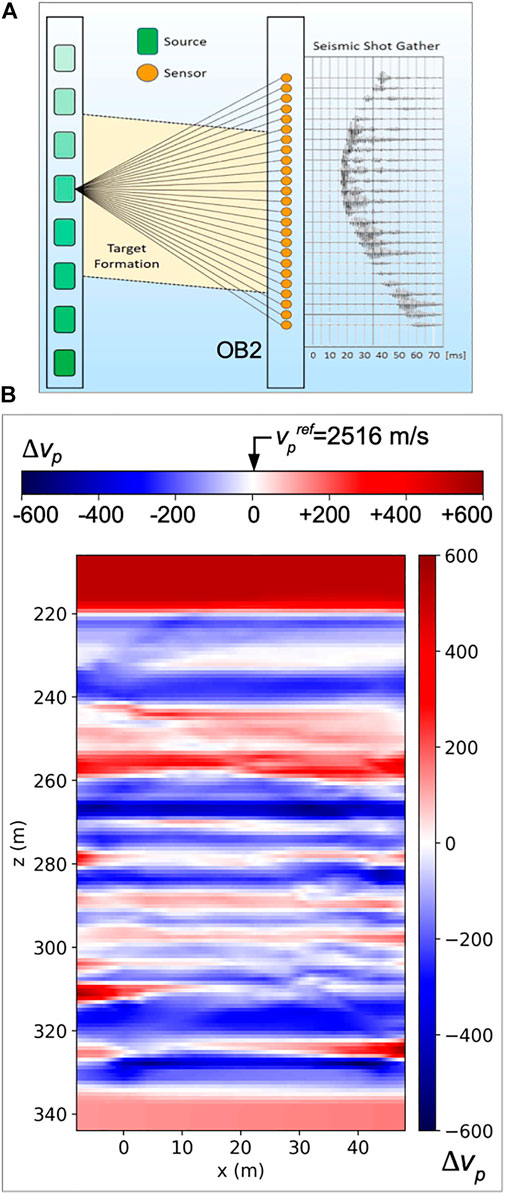
FIGURE 3. (A): Schematic view of crosswell seismic system. (B): 2D $v_p$-image resulting from CaMI.FRS seismic field data inversion. Shown velocity anomalies $\Delta v_p$ are with respect to the reference velocity $v_p^{ref}=2516$ m/s.

Both the $v_p$-logs as well as the final 2D $v_p$-image (Figure 3B) are the prior information that will contribute to the design of the parameter bounds for the field-data inversions presented below. First, we present a synthetic-data proof-of-concept in order to highlight the potential benefits of the method.

3.2 Synthetic-Data Inversion Demonstration

The following inversion experiments demonstrate the benefits of spatially variable inversion constraints. Each case compares pairs of inversions, one using constant bounds, one using variable bounds. Synthetic EM data is generated using the field geometry of the CaMI.FRS baseline EM survey. A major focus of this survey involved the testing of new sensor hardware, which led to the issue that the employed operating frequency of f = 200 Hz is not optimal in terms of image resolution. The resolution can be estimated by the ratio between the transmitter-receiver separation, $tx-rx$, over the skin-depth estimate, $\delta$ (Alumbaugh and Morrison, 1995),

$r=\frac{tx-rx}{\delta },\delta =\sqrt{\frac{2}{\omega \mu {\sigma }_0}},\omega =2\pi f(9)$

The baseline survey’s configuration at CaMI.FRS involves an average transmitter-receiver separation of $tx-rx=$ 54.5 m. Our synthetic model to be detailed further below has an averaged homogeneous background conductivity of ${\sigma }_0=0.07$ S/m, leading to the ratio r = 0.4 (assuming the magnetic permeability of free space, $\mu =1.2566\times {10}^{-6}$ H/m). Small ratios infer that the EM field wavelength associated with the excitation frequency is large compared to the scale of the target structure. Therefore, a ratio below one indicates that scattered (secondary) fields arising from a target anomaly can be expected to be small compared to the primary source field. The underlying survey layout will then suffer from low resolution capacity.

Given these two survey impediments, resolution loss due to the low source frequency and the sparse receiver array, our synthetic-data inversions aim at investigating whether target-specific parameter-bound modifications can help alleviate the resulting low imaging capacity in order to produce satisfactory plume delineations. We assume the evolution of a CO₂ plume due to an injection source near the center of the crosswell setup (Injector well in Figure 1A). Seismic imaging indicated a predominantly horizontally stratified background geology (Figure 3B). Therefore, underlying assumptions for the plume geometry involve an anisotropic hydraulic conductivity ratio that results in a greater horizontal flow and thus an ellipsoidal plume shape with the largest horizontal semiaxes along the x-axis (defining the well plane).

Our imaging studies are of a somewhat academic nature by assuming either purely electrically resistive or conductive CO₂-induced anomalies. Laboratory studies indicate that much more differentiated electrical-conductivity alterations can occur due to potentially opposing effects due to ion content versus ion mobility that depend on pore water salinity, gas concentration, pressure, and temperature (Börner et al., 2015). Here, we restrict ourselves to two distinct cases: 1) a free CO₂ phase acts as an electrical insulator and thus causes a resistive plume, and 2), at low pressures (shallow injection depths), a high ion content due to dissociation of carbonic acid results in a conductive plume.

Synthetic data generation follows the standard procedure of adding normally distributive random Gaussian noise to the real and imaginary components of the vertical magnetic fields (measured in A/m). Noise magnitudes are based upon 0.5% of the data amplitude and an additional noise floor of 10⁻¹¹ A/m. For computational savings, we further exploit the reciprocity principle by swapping out transmitters and receivers so that the receiver well hosts 8 computational transmitters. While well deviations are accounted for, no sensor rotations are considered.

3.2.1 Bounds Within Approximate Ellipsoidal Target Regions

Our underlying premise is to employ bound constraints as a way of focusing the EM imaging by exploiting prior information. Our synthetic example simulates a case where prior information exists in form of a delineation of a focus zone, which could be the product of concurrent reservoir modeling. The bound constraints thus serve as a way of augmenting the geophysical model resolution in a zone that is of hydrogeological interest.

The zone of interest in our electrical-conductivity model will be a plume of ellipsoidal shape and with anomalous electrical conductivity relative to the background. We consider two cases, a resistive and a conductive plume. The ellipsoid’s semiaxes lengths (in meters) are (a, b, c) = (18.5, 10.5, 12.5) along the axes x, y, z, and it is centered at (x, y, z) = (22, 0, 257). White contour lines in Figure 4A outline the true target geometry. The colored ellipsoidal regions that occur incongruent to this actual geometry define the volume where lower and upper inversion parameter bounds are modified with respect to constant default bounds.

FIGURE 4

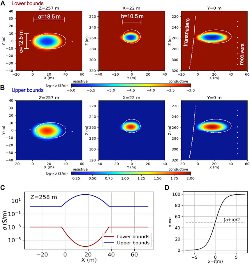
FIGURE 4. (A): Plume imaging for CaMI.FRS. Spatially variable lower and upper model parameter bounds constrain inversions for an ellipsoidal CO₂ plume. Variable bounds occur over an ellipsoid that is different in shape and center coordinates to the true plume, the latter indicated by white contours and the semiaxes lengths (a,b,c). Crosswell instrument locations are projected. Lower parameter bounds span the electrical-conductivity range from 10⁻⁶ to 10⁻³ S/m. (B): Upper bounds range from 1.5 to 100 S/m. (C): Lower and upper bounds are paired such that constraints open up when traversing the ellipsoidal target region, here shown for the x-axis at (y,z) = (0, 258) m. (D): The logarithmic transformation function of Eq. 4 is exemplified for the bound interval $\left[a,b\right]=\left[{10}^{-6},100\right]$.

A prerequisite for designing modified bound constraints would be a reservoir flow model that approximates fluid saturations and thus plume evolution. While we do not carry out such flow-modeling, it is safe to assume that, at a minimum, a basic reservoir model will exist for the majority of GCS sites. However, depending on the degree of model refinement, there will always be some uncertainty associated with operational reservoir flow predictions. The incongruity between true and assumed plume boundaries is meant to simulate this uncertainty. To quantify the deviations, we assume that predictive flow modeling would deliver a plume estimate with the erroneous ellipsoid dimensions of (a, b, c) = (20.5, 12.5, 10.5). In addition, the center point is shifted to (x, y, z) = (18, 0, 260), which shall account for actual local preferential flow paths that would exceed the complexity of the available flow model.

Lower (Figure 4A) and upper (Figure 4B) $\sigma$-parameter bounds are designed according to Eqs 5–8. As illustrated in Figure 4C, preset default bounds $\left[a^{def},b^{def}\right]=\left[{10}^{-3},1.5\right]$ expand within the plume region, up to the maximal interval $\left[a^{min},b^{max}\right]=\left[{10}^{-6},100\right]$ at the center. Figure 4D exemplifies the parameter transformation (Eqs 3, 4) that would result for this widest interval. Generally, the asymptotic curve behavior indicates the logarithmic transformation’s effect of avoiding $\sigma$-parameter over- and undershoots during the inversion process. Widening the bound interval corresponds to increasing the parameter range in which the relationship between original and transformed parameter is close to linear.

3.2.2 Inverting for Resistive and Conductive Plumes

First, we assume the simplistic case where a free CO₂ phase would act as an electrical insulator, thus causing a resistive plume. Figure 5A compares inversions using spatially constant bounds versus variable bounds. All inversions start with a homogeneous model of $\sigma =0.07$ S/m ($\approx 14.3 \text{Ω}m$). The first plot row shows the actual resistive anomaly to be imaged. It would be caused by an injection source at (x, y, z) = (22, 0, 257), creating the aforementioned ellipsoidal plume geometry (Figure 4A, white contour lines). Mimicking highest CO₂-saturation levels near the injector, $\sigma$ gradually increases from a minimum of $\sigma =2.34\times {10}^{-3}$ S/m ($\approx 427 \text{Ω}m$) at the center towards the borders where it blends with the background. The background has a generally 1D structure with minor 3D anomalies and was obtained through transforming an image of seismic velocity $v_p$ (Figure 3B) into $\rho$ through the relation

$\text{lo}{\text{g}}_{10}\left(\rho \right)=m\cdot \text{lo}{\text{g}}_{10}\left(v_p\right)+c,$

with the constants $m=3.88$ and $c=-11$. This empirical relation is chosen here arbitrarily as it was found to explain $\rho$-$v_p$ correlations for near-surface materials (Meju et al., 2003).

FIGURE 5

FIGURE 5. (A): Plume imaging for CaMI.FRS. Comparative inversions for an electrically resistive plume model. The upper, middle, and lower plot rows show, respectively, true model, inversion result using constant bounds, and inversion result using spatially variable bounds. (B): Comparative inversions for an electrically conductive plume model. The upper, middle, and lower plot rows show, respectively, true model, inversion result using constant bounds, and inversion result using spatially variable bounds. The corresponding variable lower and upper parameter bounds are shown by Figure 4. Elliptical contour lines in the images outline true (black) and assumed (green) plume boundaries. Assumed boundaries pertain to the ellipsoidal region defining the variable lower and upper parameter bounds. (C): Inversion of data set created from the background model using the variable bounds.

The 3D model outcome in Figure 5A (second plot row) results from constant parameter bounds $\left[a^{def},b^{def}\right]=\left[{10}^{-3},1.5\right]$ S/m, to be compared against the counterpart with variable bounds (third plot row). Most noticeable is the weak target anomaly reproduction in both images, which is in alignment with data sensitivity limitations. It is a general issue that VMD crosswell systems have limited capacity in resolving resistive targets that are relatively thin with respect to instrumented well sections (e.g., Grayver et al., 2014). At the same time, the inversion reproduces some of the conductive background structures, which is mostly visible in the x-z-sections of both images.

At low porewater salinities and injection levels that are shallow enough so that CO₂ remains in the gaseous state, dissociation of carbonic acid causes higher ion contents. The resulting electrically conductive plume is simulated here at the injection depth of 257 m. The corresponding model in Figure 5B (true model in first plot row) uses the same background conductivity and plume geometry as the resistive plume. Now, the conductivity decreases from a maximum of 1.7 S/m at the ellipsoid center towards the background values at the borders.

Compared to a resistive anomaly, the sensitivity of VMD systems increases for a conductive anomaly. Similar to its resistive counterpart, the inversion with constant bounds produces a plume image that remains faint (Figure 5B, second row). However, the usage of the variable bounds achieves a clearer plume delineation (third row).

3.2.3 Verification of Data Sensitivity

We emphasize that the variable-bounds concept has the mere goal of improving model resolution in terms of boosting the NLCG search process. It cannot alleviate a deficient data sensitivity. Insufficient sensitivity would cause solution instability. Preceding sensitivity studies therefore ensure that model parameters of target zones are well-resolved, regardless of any type of inversion constraints. A basic sensitivity check compares H_z-field responses calculated for the 59 receivers due to a selected source position located at z = 259 m (Figure 6). Amplitude (upper plot) and phase (lower plot) data are calculated for the background, where no ellipsoidal anomaly is present, and plotted together with the data containing the signal due to the resistive (blue lines) and conductive (red lines) plume. Percentage differences (dashed lines) between background and anomalous responses confirm that the sensitivity is higher for the conductive target (red dashed lines). While the degree of sensitivity is generally low, it is well above the assumed noise level (here 0.5%), thus validating that the sensitivity is sufficient for this kind of anomaly. Moreover, percentage differences (dashed lines) that are above noise level appear over a slightly larger depth section for phase than for amplitude. This sensitivity behavior made us set the data weights pertaining to the imaginary field component twice as high as for the real component. Since this is an arbitrary choice, it is likely that the plume imaging might be further optimized by means of additional trial inversions with proper differential data weighting.

FIGURE 6

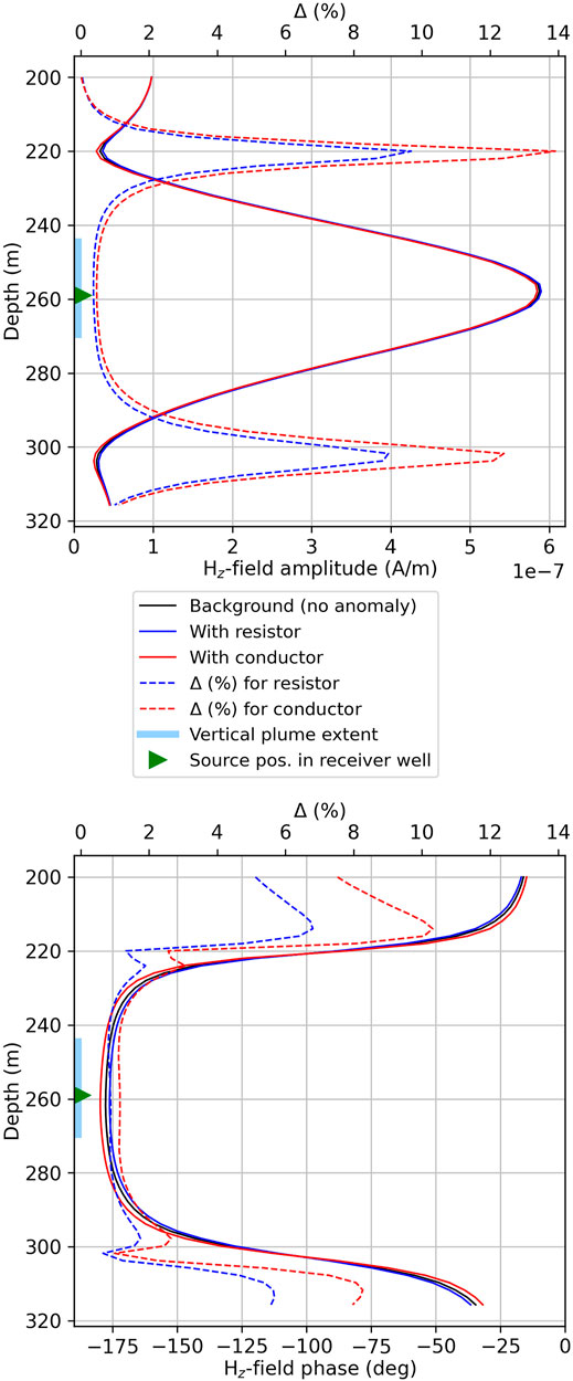
FIGURE 6. Sensitivity check in form of background-versus-anomaly forward modeling. The shown profile corresponds to one transmitter-receiver traverse. Hz-field amplitudes resulting from the background model (black lines) are compared against their counterparts calculated from the models with resistive (blue lines) and conductive (red lines) bodies. Dashed lines show percentage differences.

3.2.4 Verification of Solution Consistency

Figure 7A summarizes all four inversion instances (resistor and conductor, with constant and variable bounds) by showing the total RMS data fit against the model-updating iterations, the latter set to a maximum of 200. All inversions reach an RMS error below one. When facing generally low data sensitivities and such a similar general error convergence, the quality differences between different solutions are usually hardly discernible from individual data fits. Figure 7B exemplifies both initial and final fits produced by the variable-bound inversion for the conductive target. Here, maximal differences between the data fits at iterations 0 and 200 amount to 27% for amplitude and 31% for phase. Data fits for the corresponding constant-bound result (not shown here) are visually identical. These observations give rise to a verification of the solution consistency. Specifically, we want to ensure through two tests that 1) the anomalies are not an imaging artifact caused by the bound constraints, and 2) the solution is sufficiently independent of the starting model.

FIGURE 7

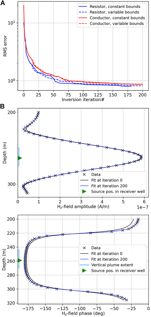
FIGURE 7. (A): Total RMS misfit for four synthetic-data inversions for a resistive and conductive plume, each comparing constant versus variable bounds. (B): Inverted data (symbols) and fits for the initial model guess (iteration 0) and the final model update (iteration 200) are shown as amplitudes and phases calculated from the vertical magnetic field. The shown profile corresponds to one transmitter-receiver traverse with its source located at z = 259 m. The vertical blue bar (left) indicates the vertical extent of the ellipsoidal plume.

The first test for solution consistency is in form of an inversion for the background model. For this check, the inverted data is calculated from the model without any anomalous ellipsoid present, that is, the data contains only the footprint of the background. At the same time, the inversion uses the variable bounds. Figure 5C shows the result of this test, where the x-y section exhibits a minor artifact reflecting the zone of the augmented bounds. However, generally, the final image indicates neither a resistive nor a conductive anomaly.

The second test verifies solution consistency over a range of starting model values. Figure 8A summarizes a sequence of 24 variable-bound inversion realizations for the conductive plume target. The starting $\sigma$ spans the range from (logarithmically) 0.013 S/m to 0.32 S/m. A simple RMS measure tracks the difference between each final model and the true model (true model shown by Figure 5B, upper row). A first observation is that the course of the RMS error does not appear erratic with changing starting $\sigma$, which would be the case for a more ill-posed inverse problem. Instead, the RMS becomes minimal within the interval $\left[{\sigma }_1,{\sigma }_2\right]$. Figure 8B shows the images for the two starting values ${\sigma }_1$ and ${\sigma }_2$. Both images contain features of the conductive target, indicating independence from the starting $\sigma$ over a range that exceeds an order of magnitude.

FIGURE 8

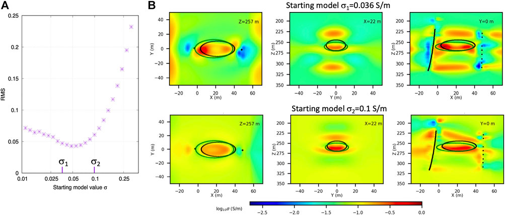
FIGURE 8. (A): Multiple inversion realizations for the conductive ellipsoidal anomaly (true model shown by Figure 5B, first row) using a range of homogeneous starting model values. The RMS error quantifies the difference between the true model and each inversion result. (B): Model reproductions exemplified for two starting-model values, ${\sigma }_1=0.036$ S/m and ${\sigma }_2=0.1$ S/m.

3.3 Field-Data Inversion for Baseline Characterization

The following demonstration applies the concept of variable bounds to the 3D inversion of a baseline (pre-injection) field data set taken at CaMI.FRS. The well geometry is as shown by Figure 1. Here, we do not apply the reciprocity principle in order to honor the deviated transmitter well. The deviation causes transmitter coil rotations. Rotations are quantified by dip and azimuth angles, where maximum angles reach, respectively, 6.9° and 27.8°. Receiver rotations are negligible. The inverted data are vertical magnetic fields recorded at 8 receivers and sourced by 59 transmitters operating at 200 Hz.

No follow-up time-lapse data set is available at the time of writing. Since the measurements only contain the footprint of the background geology, we redefine the inversion objective. Instead of mapping fluid-induced anomalies, the design of bound constraints aims at identifying potential interwell zones of interest within the background geology. We first identify the nature of these anomalous zones through a 1D zonation. Using the optimization framework provided by the PEST protocol (Doherty, 2015), a sequence of 250 independent 1D inversion realizations with different starting models is carried out. No parameter smoothing constraints are imposed. Instead, each inversion is initiated with a different $\sigma$-value of a homogeneous starting model, ranging logarithmically from 0.006 to 0.75 S/m. This range was derived from $\rho$-logs.

Figure 9 compares the $\rho$-logs against the average 1D model, the latter calculated as a simple mean from the 250 inversion realizations. Averaging over all estimated models intends to provide independence from the starting model. The model consists of 65 resistivity layer parameters with fixed thickness and an additional parameter representing the overburden. Standard deviations for the estimated layer resistivities have an average of 62% with respect to their mean, which is further evidence for a relatively low resolution. However, only the general trend is of interest. Comparing the estimated $\rho$-profile with the existing well logs exhibits a moderate degree of agreement, which is consistent with the sparse receiver coverage.

FIGURE 9

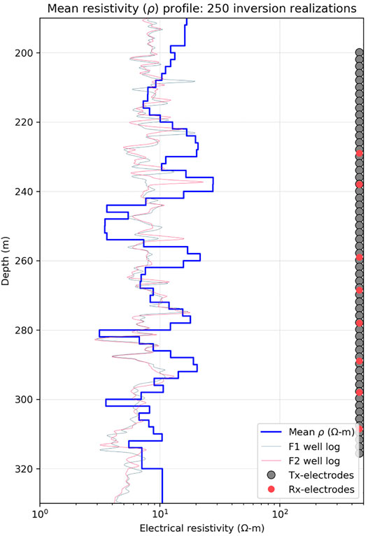
FIGURE 9. 1D resistivity well logs taken at CaMI.FRS. Also shown is the mean model calculated from 250 field-data inversion realizations. The final mean 1D model comprises parameters for 66 layers of fixed thickness. The vertical transmitter (grey) and receiver (red) electrode positions are projected onto the same line. Actual electrode distances are shown by Figure 1C.

Given that the VMD system exhibits better sensitivity towards conductive anomalies, we define the inversion objective to focus on possibly existing low-$\rho$ (conductive) zones. This choice is further based on the observation that a zone of minimum $\rho$ between z = 280 m and z = 290 m depth produced by the 1D inversion roughly coincides with the minimum in both $\rho$-logs (Figure 9). Our inversion objective is thus to probe for the potential existence of conductors that may be structurally more complex than a horizontally layered background. The existence of such structures is also indicated by a zone of low correlation in the $\rho$-logs (Figure 2A).

3.3.1 Design of Parameters Bounds From Prior Information

We outline a four-step procedure for the design of target-adapted lower and upper parameter bounds for a constrained 3D inversion. The main principle is the widening of a given default bound interval $\left[a^{def},b^{def}\right]\to \left[a^{def}-\Delta a,b^{def}+\Delta b\right]$ based on the abovementioned inversion objective. The degree of widening, quantified by $\Delta a$ and $\Delta b$, is non-zero in zones that are deemed anomalously conductive with respect to a given reference and increases with the degree of discrepancy. We reiterate that reliable prior information is important for this procedure. In our case, this information is provided by the $v_p$ and $\rho$ well logs (Figure 2A) and a 2D image of seismic velocity (Figure 3B). Figure 10 illustrates the complete procedure of bounds construction with its steps described in the following.

FIGURE 10

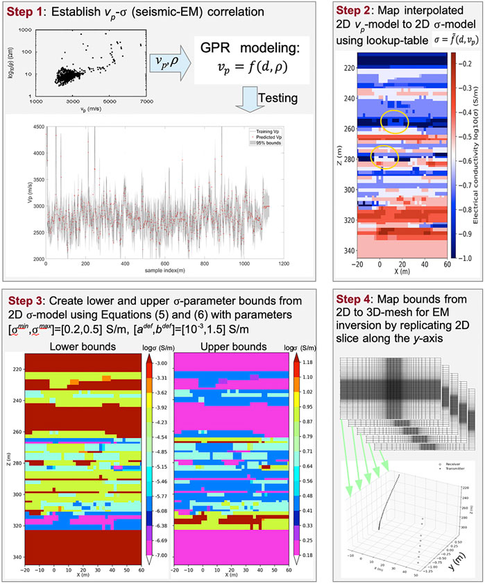
FIGURE 10. Workflow for creation of spatially variable 3D lower and upper conductivity parameter bounds for CaMI.FRS field data inversion. Lower bounds have a default (maximum) value of $a^{def}={10}^{-3}$ S/m and decrease to a minimum of $a^{min}={10}^{-7}$ S/m in predefined areas of interest. Upper bounds have a default (minimum) value of $b^{def}=1.5$ S/m and increase to a maximum of $b^{max}=15$ S/m in the same areas of interest. Ellipses (orange) in the image of Step 2 indicate regions with slight deviations from a predominantly horizontally layered structure.

3.3.1.1 Step 1: Correlating Seismic (v_p) With EM (σ) Properties

Concurrent well logs of $\rho$ and $v_p$ (Figure 2A) are the input for the construction of a $v_p$-$\sigma$ lookup table by means of a Gaussian Process Regression (GPR) model. The model establishes a relationship $v_p=f\left(d,\rho \right)$, where $d$ is the logarithmic depth and $f$ represents a multivariate Gaussian distribution. We assume a squared-exponential covariance function for the Gaussian distribution. GPR is a form of supervised machine learning (Rasmussen and Williams, 2006). Using 2/3 of the log data for training and 1/3 for testing, GPR provides confidence intervals for the test predictions of $v_p$ (Figure 10, Step 1). The testing yielded that 95.6% of all predictions lie within the predicted 95% confidence interval about the true values.

3.3.1.2 Step 2: Mapping ${\mathit{v}}_{\mathit{p}}$ to $\mathit{\sigma }$

Rearranging $v_p=f\left(d,\rho \right)$ so that we can construct a lookup table $\sigma =\tilde{f}\left(d,v_p\right)$, the $v_p$-image of Figure 3B is the input to $\tilde{f}$. The output of $\tilde{f}$ is a $\sigma$-model interpolated to the 2D grid of inversion parameters representing the crosswell plane at y = 0. This model is our prior information, ${\mathbf{m}}^{ref}={\mathit{\sigma }}^{ref}$, from which target zones of potentially anomalous ${\sigma }^{ref}$ are to be identified. Zones of coinciding low and high values in the 2D models (compare the $v_p$-image of Figure 3B to ${\mathit{\sigma }}^{ref}$ in Figure 10, Step 2) indicate the negative $v_p$-$\sigma$ correlation, which is equivalent to a positive $v_p$-$\rho$ correlation, the latter also discernible in the vertical profiles of $v_p$ and $\rho$ (Figure 2A).

3.3.1.3 Step 3: Augmenting Parameter Bounds According to Identified Anomalies

The estimated 1D model of Figure 9 guides the definition of an approximate anomaly threshold. The estimated minimum layer resistivity amounts to $min\left(\rho \right)=3.13 \text{Ω}m$, which is a lower threshold for regions of anomalously low $\rho$. To be less restrictive, our chosen objective uses an actual threshold above this limit, set to the reference $\rho =5 \text{Ω}m$. Since our inversion scheme operates on $\sigma$, the threshold becomes ${\sigma }^{min}=0.2$ S/m, where the superscript min now refers to the minimum $\sigma$ in the reference ${\mathit{\sigma }}^{ref}$ in order to qualify as anomalously conductive. The underlying inversion objective is thus to focus on local 3D anomalies that are characterized by ${\sigma }^{ref}>{\sigma }^{min}$. Therefore, all zones fulfilling ${\sigma }^{ref}>{\sigma }^{min}$ undergo a modification of a given default bound interval $\left[a^{def},b^{def}\right]=\left[{10}^{-3},1.5\right]$ according to Eqs 5, 6. Effectively, the bounds widen similar to Figure 4C. Here, the anomaly range is given by $\left[{\sigma }^{min},{\sigma }^{max}\right]=[0.2,0.5]$. For all ${\sigma }^{ref}\in \left[{\sigma }^{min},{\sigma }^{max}\right]$, Eqs 5, 6 map ${\sigma }^{ref}$ onto the corresponding augmented bound intervals, $\left[a^{min},a^{def}\right]=[{10}^{-7},{10}^{-3}]$ and $\left[b^{def},b^{max}\right]=[1.5,15]$. Note that the maximum bound interval $\left[a^{min},b^{max}\right]$ holds for all parameters ${\sigma }^{ref}\ge 0.5$. The outcome is a set of variable lower and upper bounds as shown in Figure 10 (Step 3). These bounds remain fixed during the inversion process.

Note that augmented bounds cover the majority of the inversion domain, that is, in contrast to the central target given by the ellipsoid in Figure 4A, the bounds do not reflect a narrow focus zone. Also, we reiterate that while bound construction is based on prior assumptions about anomalously high $\sigma$, the widening of the bounds in both directions will allow for both conductive and resistive anomalies in the imaging.

3.3.1.4 Step 4: Expand Parameter Bounds to 3D Grid

The bounds are discretized on the 2D x-z plane at y = 0. The 2D grid is replicated along all grid nodes of the y-axis in preparation for the subsequent 3D inversion. We choose 3D over 2D inversions based on earlier comparative studies on 2D versus 3D inversion of data containing actual 3D signatures. These studies have raised the concern that in the presence of actual 3D structures, the restriction to two model dimensions can lead to image artifacts (Papadopoulos et al., 2007; Nimmer et al., 2008; Hübert, 2012; Feng et al., 2014). To further limit potential artifacts, it is preferable to retain the actual 3D well deviations that are contained in the data.

3.3.2 Comparative 3D Field-Data Inversion

Two comparative field data inversions employ the constant bounds $\left[a^{min},b^{max}\right]=\left[{10}^{-7},15\right]$ and the variable bounds created through the mapping scheme described above (Figure 10). The initial reasoning for choosing a very wide constant-bound interval was to let the inversion practically be unbounded in order to avoid any bias due to potentially too tight bounds. However, other constant-bound inversions not reported here experimented with narrower intervals which yielded no significant difference in the final image.

The initial model guess for both inversions is given by the final mean 1D model of Figure 9 (referred to as 1D model in the following). One could assume that the $v_p$-$\sigma$ lookup table that comes out of the GPR modeling provides a better starting $\sigma$-model (Figure 10, Step 2) as it combines the layered geology with local inhomogeneities. However, we employ this model merely for the identification of conductive anomalies and the corresponding bound modifications. Its values span a range that exceeds the $\sigma$-range of the resistivity logs and 1D model by an order of magnitude, which would result in a much greater initial RMS misfit.

The low final RMS misfit error of 1.78 achieved by the 1D model equals the starting RMS for the 3D inversions, confirming the dominating layered structure of the geology suggested by Um et al. (2020). Figure 11A summarizes the total error convergence. The variable-bound 3D inversion converges to a slightly lower final RMS and reaches the preset maximum iteration number (250), while the constant-bound inversion terminates after 173 iterations. However, final data fits are visually practically identical for both inversions, as evident in fits exemplified for one selected source depth (Figure 11B).

FIGURE 11

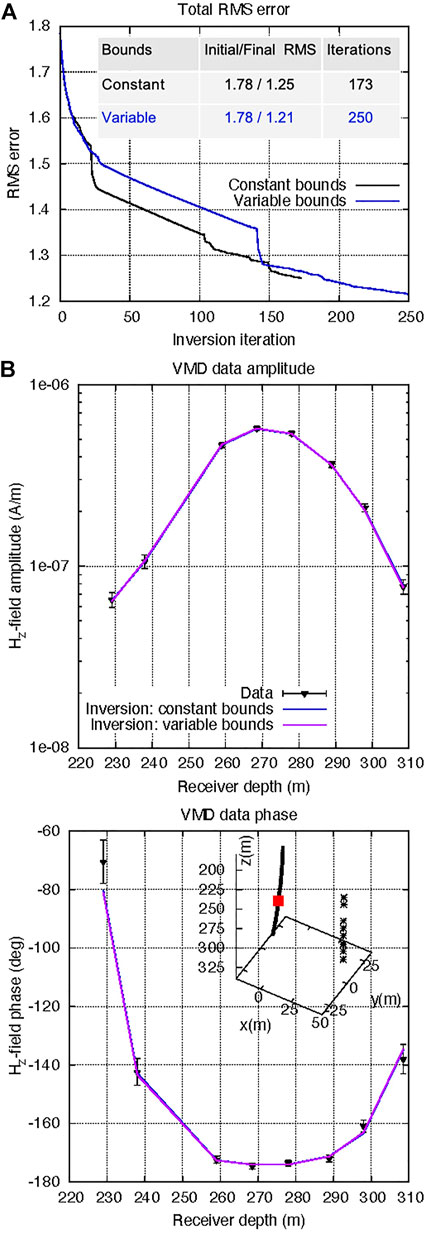
FIGURE 11. (A): Total RMS fitting error for CaMI.FRS field data inversion. (B): Data (symbols) and fits for inversions with constant bounds (blue lines) and variable bounds (purple lines). Real and imaginary vertical-magnetic fields are converted into amplitude and phase. The exemplified fits correspond to one transmitter-receiver traverse with the source located at z = 270 m (marked by red symbol).

It is now of interest to what degree variable bounds contribute to a better target inversion. While synthetic-data trials make an assessment straightforward, the absence of a ground truth in field-data inversions makes us revert to examining model differences. Figure 12 shows relative $\sigma$-differences with respect to a reference. First, we want to visualize the difference $\Delta {\sigma }_{var}=M_{var}^{3D}-M^{1D}$ between the final variable-bound inversion result ($M_{var}^{3D}$) and the starting 1D model ($M^{1D}$). Deviations from a horizontally layered structure that are within the center plane of the interwell region are most pronounced within a zone between z = 240 m and z = 260 m (Figure 12A). Moreover, the image $\Delta {\sigma }_{var}$ strongly resembles $\Delta {\sigma }_{con}=M_{con}^{3D}-M^{1D}$, where $M_{con}^{3D}$ is the final constant-bound inversion result. Instead of $\Delta {\sigma }_{con}$, Figure 12B shows the difference $\Delta \sigma =M_{var}^{3D}-M_{con}^{3D}$. Absolute differences are relatively small, indicating no significant bias due to the variable-bound constraints. Further, positive differences dominate within the well plane, which translates to $\sigma \left(M_{var}^{3D}\right)>\sigma \left(M_{con}^{3D}\right)$. These observations point to some degree of significance for anomalies characterized by $\Delta \sigma >0$ that deviate from a horizontally layered geology within the zone z = 240–260 m.

FIGURE 12

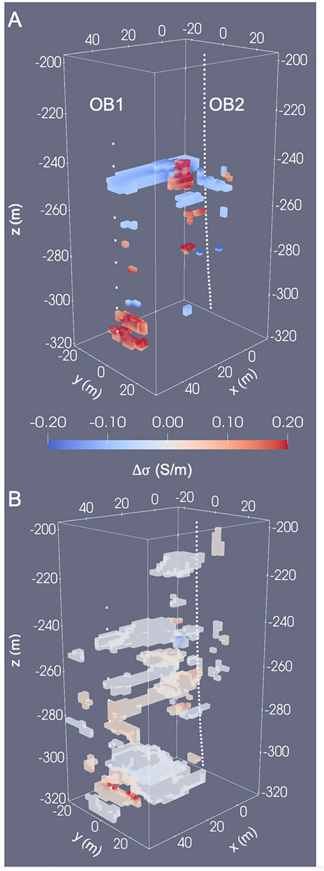
FIGURE 12. (A): Inversion of CaMI.FRS field data with variable parameter bounds. The inversion is initialized with the layered starting model ($M^{1D}$) obtained from 1D inversion (Figure 9). Shown are deviations $\Delta {\sigma }_{var}=M_{var}^{3D}-M^{1D}$ where $M_{var}^{3D}$ is the final model update. Only deviations $\left|\text{Δ}\sigma \right|>0.075$ S/m are visualized, where blue and red regions indicate conductivity decreases and increases, respectively, with respect to the starting model. (B): Comparative inversion of CaMI.FRS field data. Shown is the difference $\text{Δ}\sigma =M_{var}^{3D}-M_{con}^{3D}$, calculated from the final model updates using variable ($M_{var}^{3D}$) and constant ($M_{con}^{3D}$) bounds. Only deviations $\left|\Delta \sigma \right|>0.005$ S/m are visualized, where blue and red regions indicate negative and positive differences, respectively.

4 Discussion

Parameter constraints in form of spatially variable lower and upper bounds provide a straightforward way of incorporating spatial prior model information pointing to focus zones in an inversion workflow. Contrary to the common way of scaling the width of model parameter bounds with the uncertainty of prior information, we simply enlarge bounds in zones that host anticipated anomalies. The main purpose of prior information then reduces to the delineation of anomaly boundaries, without the need to quantify absolute properties exactly. While they cannot improve the lack of data sensitivity, widened bound intervals are a means of selectively increasing model fidelity in target zones. The approach essentially translates to scaling and steering the NLCG inversion’s search procedure in the model space so that local solution minima are more likely to be circumvented. It can accelerate solution convergence.

In time-lapse imaging related to GCS, reservoir flow modeling would provide the spatial a priori information for the design of location-dependent parameter bounds. Given that reservoir modeling of injection-induced hydrogeological state changes will likely accompany future GCS site management, it represents an inexpensive source of auxiliary information for constraining geophysical plume imaging. One may thus call the presented method a “poor people’s” alternative to a more sophisticated coupling by means of hydrogeophysical joint inversion; the latter would involve inverse modeling of a flow system interlinked with the EM data simulation (e.g., Commer et al., 2020).

In light of foreseeable economic limitations of long-term CCS monitoring, our synthetic-data study mimicked some inhibiting factors that actually occurred in the field. These are a suboptimal source frequency and resolution loss due to an incomplete data set. Despite these imposed shortcomings, fluid-induced conductivity alterations could still be mapped, suggesting that the variable-bounds concept can serve as a means to offset model resolution loss due to defective survey coverage to some degree.

Inversions with variable bounds applied to the CaMI.FRS baseline field data highlight that geophysical prior information, here seismic imaging and well logs, can be utilized for the design of target-specific parameter bounds. The presented inversions lend weight to indicators for correlated anomalies between $\sigma$ and $v_p$. These indicators are 1) a zone of anomalously high $v_p$ between z = 240 m and z = 260 m in the seismic image (Figure 3B), and 2) the occurrence of 3D positive conductivity deviations from the 1D background within the same depth section of the well plane (Figure 12A). Note that a low correlation between the $\rho$-logs of wells OB1 and OB2 in the same depth section (Figure 2A) already indicated such non-1D structures. Concurrently, while less significant, deviations with positive $\Delta \sigma$ from a 1D structure also appear in the $\sigma$-image derived from the $v_p$-$\sigma$ correlation (Figure 10, Step 2, regions of $\Delta \sigma >0$ indicated by orange circles).

A final remark is that, as common in geophysical inversion problems of an underdetermined nature, multiple trial-and-error inversion realizations may be necessary to reduce the uncertainties of these results. Inversions might be further improved through optimized function parameters that control the spatial bound variation. In cases with a prohibitively large number of inversion realizations, Bayesian optimization with inequality constraints as presented by Gardner et al. (2014) might be a feasible alternative.

Data Availability Statement

The raw data supporting the conclusion of this article will be made available by the authors, without undue reservation.

Author Contributions

MC: Writing, Editing, Conceptualization, Methodology. DA: Editing, Data acquisition, Supervision. GH: Methodology (GPR modeling). DV and PM: Methodology (seismic imaging). MW, EN, and EU: Data acquisition. MM: Project administration.

Funding

This research was supported by the U.S. Department of Energy, National Energy Technology Laboratory, CCSMR program, under the U.S. DOE Contract No. DE-AC02-05CH11231.

Conflict of Interest

The author MM is employed by Carbon Management Canada. The author PM was employed by Silixa Ltd.

The remaining authors declare that the research was conducted in the absence of any commercial or financial relationships that could be construed as a potential conflict of interest.

Publisher’s Note

All claims expressed in this article are solely those of the authors and do not necessarily represent those of their affiliated organizations, or those of the publisher, the editors and the reviewers. Any product that may be evaluated in this article, or claim that may be made by its manufacturer, is not guaranteed or endorsed by the publisher.

Acknowledgments

We thank Don Lawton, the CaMI Consortium, and all their partners for site access and the help received during field activities.

References

Abubakar, A., Habashy, T. M., Druskin, V. L., Knizhnerman, L., and Alumbaugh, D. (2008). 2.5D Forward and Inverse Modeling for Interpreting Low-Frequency Electromagnetic Measurements. Geophysics 73, F165–F177. doi:10.1190/1.2937466

CrossRef Full Text | Google Scholar

Abubakar, A., Habashy, T. M., Li, M., and Liu, J. (2009). Inversion Algorithms for Large-Scale Geophysical Electromagnetic Measurements. Inverse Probl. 25, 123012. doi:10.1088/0266-5611/25/12/123012

CrossRef Full Text | Google Scholar

Aghamiry, H. S., Gholami, A., and Operto, S. (2019). Implementing Bound Constraints and Total-Variation Regularization in Extended Full Waveform Inversion with the Alternating Direction Method of Multiplier: Application to Large Contrast Media. Geophys. J. Int. 218, 855–872. doi:10.1093/gji/ggz189

CrossRef Full Text | Google Scholar

Alumbaugh, D. L., and Morrison, H. F. (1995). Monitoring Subsurface Changes over Time with Cross-Well Electromagnetic Tomographyt1. Geophys Prospect 43, 873–902. doi:10.1111/j.1365-2478.1995.tb00286.x

CrossRef Full Text | Google Scholar

Börner, J. H., Herdegen, V., Repke, J.-U., and Spitzer, K. (2015). The Electrical Conductivity of CO2-bearing Pore Waters at Elevated Pressure and Temperature: a Laboratory Study and its Implications in CO2storage Monitoring and Leakage Detection. Geophys. J. Int. 203, 1072–1084. doi:10.1093/gji/ggv331

CrossRef Full Text | Google Scholar

Commer, M., and Newman, G. A. (2008). New Advances in Three-Dimensional Controlled-Source Electromagnetic Inversion. Geophys. J. Int. 172, 513–535. doi:10.1111/j.1365-246X.2009.04216.x10.1111/j.1365-246x.2007.03663.x

CrossRef Full Text | Google Scholar

Commer, M., Pride, S. R., Vasco, D. W., Finsterle, S., and Kowalsky, M. B. (2020). Imaging of a Fluid Injection Process Using Geophysical Data - a Didactic Example. Geophysics 85, W1–W16. doi:10.1190/geo2018-0787.1

CrossRef Full Text | Google Scholar

de Groot‐Hedlin, C., and Constable, S. (2004). Inversion of Magnetotelluric Data for 2D Structure with Sharp Resistivity Contrasts. Geophysics 69, 78–86. doi:10.1190/1.1649377

CrossRef Full Text | Google Scholar

Doherty, J. (2015). Calibration and Uncertainty Analysis for Complex Environmental Models. Brisbane, Australia: Watermark Numerical Computing.

Google Scholar

Farquharson, C. G., Ash, M. R., and Miller, H. G. (2008). Geologically Constrained Gravity Inversion for the Voisey's Bay Ovoid Deposit. Lead. Edge 27, 64–69. doi:10.1190/1.2831681

CrossRef Full Text | Google Scholar

Feng, D.-s., Dai, Q.-w., and Xiao, B. (2014). Contrast between 2D Inversion and 3D Inversion Based on 2D High-Density Resistivity Data. Trans. Nonferrous Metals Soc. China 24, 224–232. doi:10.1016/s1003-6326(14)63051-x

CrossRef Full Text | Google Scholar

Gao, G., Alumbaugh, D., Zhang, P., Zhang, H., Levesque, C., Rosthal, R., et al. (2008). “Practical Implications of Nonlinear Inversion for Cross-Well Electromagnetic Data Collected in Cased-Wells,” in Paper Presented at the 78th SEG Annual Meeting, Las Vegas, NV, November 9-14.

Google Scholar

Gardner, J. R., Kusner, M. J., Zhixiang, X., Weinberger, K. Q., and Cunningham, J. P. (2014). “Bayesian Optimization with Inequality Constraints,” in Proc. of the 31st Int. Conf. Machine Learning, Beijing, 937–945.32

Google Scholar

Grayver, A. V., Streich, R., and Ritter, O. (2014). 3D Inversion and Resolution Analysis of Land-Based CSEM Data from the Ketzin CO2 Storage Formation. Geophysics 79, E101–E114. doi:10.1190/geo2013-0184.1

CrossRef Full Text | Google Scholar

Habashy, T. M., and Abubakar, A. (2004). A General Framework for Constraint Minimization for the Inversion of Electromagnetic Measurements. Pier 46, 265–312. doi:10.2528/PIER03100702

CrossRef Full Text | Google Scholar

Haber, E., Horesh, L., and Tenorio, L. (2010). Numerical Methods for the Design of Large-Scale Nonlinear Discrete Ill-Posed Inverse Problems. Inverse Probl. 26, 025002. doi:10.1088/0266-5611/26/2/025002

CrossRef Full Text | Google Scholar

Hübert, J. (2012). From 2D to 3D Models of Electrical Conductivity Based upon Magnetotelluric Data, Experiences from Two Case Studies (Sweden: Uppsala University). Ph.D. Thesis.

Iwuagwu, C. J., and Lerbekmo, J. F. (1982). The Petrology of the Basal Belly River Sandstone Reservoir, Pembina Field, Alberta. Bull. Can. Petroleum Geol. 30, 187–207. doi:10.35767/gscpgbull.30.3.187

CrossRef Full Text | Google Scholar

Jackson, D. D. (1979). The Use of A Priori Data to Resolve Non-uniqueness in Linear Inversion. Geophys. J. Int. 57, 137–157. doi:10.1111/J.1365-246X.1979.TB03777.X

CrossRef Full Text | Google Scholar

Kim, H. J., and Kim, Y. (2011). A Unified Transformation Function for Lower and Upper Bounding Constraints on Model Parameters in Electrical and Electromagnetic Inversion. J. Geophys. Eng. 8, 21–26. doi:10.1088/1742-2132/8/1/004

CrossRef Full Text | Google Scholar

Kim, H. J., Song, Y., and Lee, K. H. (1999). Inequality Constraint in Least-Squares Inversion of Geophysical Data. Earth Planet Sp. 51, 255–259. doi:10.1186/BF03352229

CrossRef Full Text | Google Scholar

Luenberger, D. (1984). Linear and Nonlinear Programming. 2nd edition. Boston, Massachusetts, United States: Addison-Wesley.

Google Scholar

Mackie, R. L., and Madden, T. R. (1993). Three-dimensional Magnetotelluric Inversion Using Conjugate Gradients. Geophys. J. Int. 115, 215–229. doi:10.1111/j.1365-246X.1993.tb05600.x

CrossRef Full Text | Google Scholar

Medeiros, W. E., and Silva, J. B. C. (1996). Geophysical Inversion Using Approximate Equality Constraints. Geophysics 61, 1678–1688. doi:10.1190/1.1444086

CrossRef Full Text | Google Scholar

Meju, M. A., Gallardo, L. A., and Mohamed, A. K. (2003). Evidence for Correlation of Electrical Resistivity and Seismic Velocity in Heterogeneous Near-Surface Materials. Geophys. Res. Lett. 30, 1373. doi:10.1029/2002GL016048

CrossRef Full Text | Google Scholar

Menke, W. (2018). Geophysical Data Analysis: Discrete Inverse Theory. New York: Academic Press.

Google Scholar

Newman, G. A., and Alumbaugh, D. L. (2000). Three-dimensional Magnetotelluric Inversion Using Non-linear Conjugate Gradients. Geophys. J. Int. 140, 410–424. doi:10.1046/j.1365-246x.2000.00007.x

CrossRef Full Text | Google Scholar

Nimmer, R. E., Osiensky, J. L., Binley, A. M., and Williams, B. C. (2008). Three-dimensional Effects Causing Artifacts in Two-Dimensional, Cross-Borehole, Electrical Imaging. J. Hydrology 359, 59–70. doi:10.1016/j.jhydrol.2008.06.022

CrossRef Full Text | Google Scholar

Ogarko, V., Giraud, J., Martin, R., and Jessell, M. (2021). Disjoint Interval Bound Constraints Using the Alternating Direction Method of Multipliers for Geologically Constrained Inversion: Application to Gravity Data. Geophysics 86, G1–G11. doi:10.1190/GEO2019-0633.1

CrossRef Full Text | Google Scholar

Papadopoulos, N. G., Tsourlos, P., Tsokas, G. N., and Sarris, A. (2007). Efficient ERT Measuring and Inversion Strategies for 3D Imaging of Buried Antiquities. Near Surf. Geophys. 5, 349–361. doi:10.3997/1873-0604.2007017

CrossRef Full Text | Google Scholar

Rasmussen, C. E., and Williams, C. K. I. (2006). Gaussian Processes for Machine Learning. Boston, MA: The MIT Press.

Google Scholar

Sosa, A., Velasco, A. A., Velazquez, L., Argaez, M., and Romero, R. (2013). Constrained Optimization Framework for Joint Inversion of Geophysical Data Sets. Geophys. J. Int. 195, 1745–1762. doi:10.1093/gji/ggt326

CrossRef Full Text | Google Scholar

Um, E. S., Marchesini, P., Wilt, M., Nichols, E., Alumbaugh, D. L., Vasco, D., et al. (2020). “Joint Use of Crosswell EM and Seismic for Monitoring CO₂ Storage at the Containment and Monitoring Institute Field Site (CaMI): Baseline Surveys and Preliminary Results,” in Paper Presented at the 90th SEG Annual Meeting, Houston, TX, October 11-14.

Google Scholar

Vasco, D. W., and Nihei, K. (2019). Broad Band Trajectory Mechanics. Geophys. J. Int. 216, 745–759. doi:10.1093/gji/ggy435

CrossRef Full Text | Google Scholar

Wu, X., and Habashy, T. M. (1994). Influence of Steel Casings on Electromagnetic Signals. Geophysics 59, 378–390. doi:10.1190/1.1443600

CrossRef Full Text | Google Scholar

Yi, M. J., Kim, J. H., and Chung, S. H. (2003). Enhancing the Resolving Power of Least‐squares Inversion with Active Constraint Balancing. Geophysics 68, 931–941. doi:10.1190/1.1581045

CrossRef Full Text | Google Scholar