Non-Parametric Simultaneous Reconstruction and Denoising via Sparse and Low-Rank Regularization

Spatial irregular sampling and random noise are two important factors that restrict the accuracy of seismic imaging. Seismic wavefield reconstruction and denoising based on sparse representation are two popular antidotes to these two inevitable issues, respectively. This article presents a non-parametric simultaneous reconstruction and denoising via sparse and low-rank regularization that dealt with the prestack gathers efficiently and automatically. The proposed method makes no additional prior assumptions on original data other than that the seismic signal is compressible. The key parameters estimation adopts a data-driven framework without person-dependent intervention. The basic idea of the approach is to combine the two related algorithms. Thus, the sparse decomposition needs to be performed only once. We first extract the solution matrix via Fourier dictionary and then perform the reconstruction and denoising successively in the sparse domain. Obtaining a perfect interpolation result requires that the seismic data satisfy the Shannon–Nyquist sampling theorem. However, data with steep-dip events or gaps, which cannot be adequate for the procedure, are a challenge that must be faced. This work proposes to deal with the common-offset gathers, which is characterized by flat, even approximate horizontal events, to handle the under-sampling obstacle. Another excellent property of the common-offset gathers is the simple and periodic repetitive texture structure, which can be represented sparsely and accurately by the Fourier dictionary. Thus, the computational complexity of the sparse representation is reduced. Both synthetic and practical applications indicate that our algorithm is efficient and effective.

1 Introduction

Seismic data are inevitably corrupted by missing traces and random noise in field procedures, which often lead to the low signal-noise ratio (SNR), irregular sampling, and even anomalies, such as spatial aliasing and acquisition footprints. Defect data may cause severe consequences in subsequent processing flows, that is, velocity analysis, normal moveout (NMO) correction, migration, amplitude-versus-offset (AVO) analysis, and seismic attributes extraction. Hence, seismic wavefield reconstruction conjugation with denoising play fundamental roles in data analysis. This article proposes using tools in compressed sensing to solve both interpolation and noise reduction.

However, due to parameter tuning and computational complexity, wavefield reconstruction and denoising are usually regarded as two independent seismic processing flows, even though they share common calculation steps and algorithms, such as sparse decomposition. The target of the seismic wavefield reconstruction is to provide a uniformly sampled data cube. The reconstruction problem has received sufficient study. The previous works addressing this problem can be classified into four categories: wave equation-based interpolation (Ronen 1987), matrix or tensor completion (Kreimer et al., 2013; Chen et al., 2016a; Siahsar et al., 2017; Zhang et al., 2017), deep learning- (Jia and Ma 2017; Oliveira et al., 2018; Wang et al., 2018) and (Cao et al., 2020) compressed sensing-based interpolation. Among them, the compressed sensing-based method has received widespread attention due to its low computational cost. The recorded seismic data can be interpreted as a random sampling of the complete seismic data. Therefore, the problem of seismic data interpolation can be formulated as an inverse problem. Many algorithms have been introduced such as non-equispaced curvelet transform-based method, which processes irregularly sampled data gather by gather (Hennenfent et al., 2010); piecewise random subsampling scheme solved by L₁-norm constrained trust region method (Wang et al., 2011); weighted L₁-norm minimization-based wavefield reconstruction (Mansour et al., 2013), which suggests interpolating 2D partitions of the seismic line instead of the 3D cube to save computer memory (Chen et al., 2019a). reviewed the state-of-the-art interpolation models and their theoretical implications. Curvelet reconstructs the time slices by linearized Bregman method (Zhang et al., 2019); this approach can effectively handle non-uniformly sampled seismic data. The constrained optimization algorithm is an integral part of the reconstruction problem, and algorithms that can solve large-scale sparse representation are desirable. Many different algorithms have been proposed, such as orthogonal matching pursuit (OMP), alternating direction method of multipliers (ADMM) (Lu et al., 2018), Nesterov’s algorithm (NESTA) (Becker et al., 2011), spectral projection gradient method (SPGL1) (van den Berg and Friedlander 2008), and linearized Bregman method (Yin 2010). In seismic wavefield reconstruction, the dictionaries for sparse representation are often fast operators. Matrix-free and scale well algorithms, that is, SPGL1 and linearized Bregman, should be required to enable sparse representation for extremely large-scale reconstruction problems.

Random noise suppression attempts to improve the SNR of seismic data with the ultimate aim to improve imaging accuracy (Anvari et al., 2017; Chen et al., 2017) classified the denoising methods into four categories: predictive filtering-based (Chen and Ma 2014), decomposition-based (Gómez et al., 2019), sparse transform-based (Deng et al., 2017; Yuan et al., 2018; Chen et al., 2019b), and rank reduction-based (Chen et al., 2017; Anvari et al., 2019; Wang et al., 2019) seismic denoising. The principles of random noise suppression of all categories are that the statistical characteristics or propagation laws of signal and noise are different in a specific domain. Among them, low rank-based approach is an important category and consistent with the hypothesis that the seismic signal is low-rank in specific domains (Ma 2013; Anvari et al., 2017). Based on this property, noise and the useful signal can be separated by low-rank matrix or tensor decomposition in a specific domain, that is, Hankel (Wang et al., 2019) and synchrosqueezed wavelet (Anvari et al., 2017, 2019) transform. Another appealing low-rank–based denoising is the singular value thresholding (SVT) (Zhou and Zhang 2017) and its variants (Bekara and Van der Baan 2007; Chiu and Howell 2008), which is elegant and flexible and can be used in different steps of seismic signal processing. A vital issue in SVT is how much shrinkage should be imposed. Improper shrinkage may result in large bias or high variance (Candes et al., 2013). Luckily, Candes et al. (2013) proposed an unbiased risk estimate for SVT based on Stein’s unbiased risk estimate (SURE).

Simultaneous reconstruction and denoising of multichannel seismic data is not a new topic. A lot of published literature targeting solving the two problems at the same time have been published. The clean prestack cube is inherently low-rank in the f-x domain and other transform domains. When missing-traces are encountered and corrupted by random noise, the defective seismic data’s rank is inevitably increasing. Rank reduction and low-rank decomposition have been developed to overcome these two problems. Typical studies include: Oropeza and Sacchi (2011) proposed a rank reduction algorithm based on multichannel singular spectrum analysis (MSSA) and can be easily implemented by singular value decomposition (SVD). Instead of organizing spatial data into block Hankel matrixes (Kreimer and Sacchi 2012), rank-reduction to the fourth-order seismic tensor via higher-order singular value decomposition (HOSVD) was applied (Ely et al., 2015), and a 5D completion and denoising based on a complexity-penalized algorithm and tensor singular value decomposition (tSVD) was proposed. The method needs to tune only one regularization parameter. Sternfels et al. (2015) show that the method of joint low-rank and sparse inversion is suitable for random and erratic noise. To deal with the extremely noisy cube, Chen et al. (2016b) introduced a damped rank-reduction method to formulate the Cadzow rank-reduction and proposed a 5-D reconstruction and denoising method.

In this article, a practical implementation of simultaneous reconstruction and denoising was presented, which is parameter-free and can be solved via sparse and low-rank regularization efficiently. The contributions of this article are four-fold. First, the classic simultaneous denoising and interpolation algorithm map the seismic data to a high-dimensional (4D or 5D) tensor and are computationally intensive. The new method only involves matrix operations instead of handling tensor and extracting the coefficient matrix only once. Second, the parameters are adaptively obtained and do not need to be tuned manually. Third, the work demonstrated by experiments that compare to common mid-point (CMP), common-shot gathers, and common-offset gathers strategy enjoys its anti-aliasing ability and is bright to handle the under-sampling obstacle. Fourth, the sparse representation of common-offset gather via the Fourier dictionary is accurately enough and computationally inexpensive compared to the curvelet dictionary.

2 Methodology

2.1 Problem Formulation

Seismic data have two dimensions of time and space. The seismic traces are usually uniformly sampled in the temporal domain, and the Nyquist–Shannon sampling theorem is satisfied. However, due to existing obstacles and economic restrictions, there is always missing traces in seismic data, resulting in non-uniformly sampled, even aliased in the spatial domain. Moreover, seismic data are inevitably polluted by random noise. Complete and clean seismic data need to be reconstructed from recorded noisy and incomplete seismic data.

The relationship between the recorded seismic data and the complete data can be formalized as:

$\mathbf{y}=\mathbf{Lx},(1)$

where y and x are the recorded (incomplete) seismic data and complete data, respectively. Both y and x are constructed by arranging all the traces of the recorded (Y) and complete (X) data matrix into vectors. L represents the measurement matrix, which is a block diagonal matrix and is defined as $\mathbf{L}=\left[\begin{array}{llllll}\mathbf{I}\hfill & \hfill & \hfill & \hfill & \hfill & \hfill \\ \hfill & \mathbf{I}\hfill & \hfill & \hfill & \hfill & \hfill \\ \hfill & \hfill & \mathbf{0}\hfill & \hfill & \hfill & \hfill \\ \hfill & \hfill & \hfill & \mathbf{I}\hfill & \hfill & \hfill \\ \hfill & \hfill & \hfill & \hfill & \ddots \hfill & \hfill \\ \hfill & \hfill & \hfill & \hfill & \hfill & \mathbf{I}\hfill \end{array}\right]$ (each 0 represents a missing trace, and each I represents a recorded seismic trace).

It should note that both y and x are infected by random noise. The purpose of the proposed method is to reconstruct the expected clean and complete data ${\mathbf{x}}^{\ast }$ from y. Solving Eq. 1 can only give rise to complete noisy data. However, worse still, seismic wavefield reconstruction aims to recover a high-dimensional signal cube from a smaller number of measurements. formula (1) is underdetermined and has infinitely many solutions. The proposed countermeasure to address these two bottlenecks will be described in detail in the following subsections.

2.2 Simultaneous Reconstruction and Denoising in the Sparse Domain

It is possible to reconstruct sparse signals from highly incomplete sets, which can be done by sparse representation. The seismic data are compressible and sparse in the curvelet and Fourier domains. The sparsity adds effective constraints to the underdetermined inverse problem, thereby reducing the distress of the multiplicity. So, an effective strategy for the underdetermined problem (1) is that we can transform x into the Fourier or curvelet domain (as shown in Eq. 2) and then formulate the reconstruction problem as an L₁-norm regularization (as shown in Eq. 3) (Mansour et al., 2013).

$\mathbf{y}=\mathbf{Am},\mathbf{A}=\mathbf{L}{\mathbf{F}}^H,(2)$

where F is a sparsifying operator; that is, Fourier or curvelet transform, m is the Fourier or curvelet coefficient, and superscript H represents the conjugate transpose.

$\arg \underset{\mathbf{m}}{\min }{\Vert \mathbf{m}\Vert }_1\mathrm{ }s.t.\mathrm{ }{\Vert \mathbf{y}-\mathbf{Am}\Vert }_2^2\le \epsilon ,(3)$

where ${\Vert \cdot \Vert }_1$ and ${\Vert \cdot \Vert }_2$ denote L₁- and L₂-norms, respectively; ε is a fitting error. We have learned that Eq. 3 is a basis pursuit denoise (BPDN) problem; it can be optimized by the spectral projection gradient method. However, L₁-norm is non-differentiable and the augmented model for Eq. 2 is adopted (Yin 2010):

${\mathbf{m}}^{\ast }=\arg \underset{\mathbf{m}}{\min }{\Vert \mathbf{m}\Vert }_1+\frac{1}{2\alpha }{\Vert \mathbf{m}\Vert }_2\mathrm{ }s.t.\mathrm{ }{\Vert \mathbf{y}-\mathbf{Am}\Vert }_2^2\le \epsilon ,(4)$

where typically $\alpha =1$.

Solving Eq. 4 can only get complete noisy data, that is, ${\mathbf{m}}^{\ast }$ is corrupted by noise. Consequently, the next step is to denoise the reconstruction ${\mathbf{m}}^{\ast }$. We first rearrange ${\mathbf{m}}^{\text{*}}$ into a 2D matrix M.

Due to the repetitive texture structure, the prestack seismic gathers are low-rank matrixes (Ma 2013). In a transformed domain, that is, Fourier and curvelet domains, the coefficient matrix M is also characterized by the low-rank feature (Nazari Siahsar et al., 2016). Suppose M is sullied by Gaussian noise, we have the noisy coefficient matrix M about a clean low-rank matrix ${\mathbf{M}}_{\text{den}}$ of interest. A natural approach to this problem is singular value thresholding (SVT), which formalizes noise suppression as:

${\mathbf{M}}_{\text{den}}=\mathrm{SV}{\mathrm{T}}_{\lambda }\left(\mathbf{M}\right)=\arg \underset{{\mathbf{M}}_{\text{den}}}{\min }\lambda \mathrm{rank}\left({\mathbf{M}}_{\text{den}}\right)+\frac{1}{2}{\Vert \mathbf{M}-{\mathbf{M}}_{\text{den}}\Vert }_F^2,(5)$

where ${\Vert \cdot \Vert }_F$ is the Frobenius norm and $\mathbf{M}=\mathbf{U\Sigma }{\mathbf{V}}^H$ ($\mathbf{U}=\left[{\mathbf{u}}_1,{\mathbf{u}}_2,\cdots {\mathbf{u}}_n\right]$ and $\mathbf{V}=\left[{\mathbf{v}}_1,{\mathbf{v}}_2,\cdots {\mathbf{v}}_n\right]$ are left and right singular vectors, respectively; $\mathbf{\Sigma }=diag\left({\sigma }_1,{\sigma }_2,\cdots ,{\sigma }_n\right)$ is a diagonal matrix with singular values of M on its diagonal) is the singular value decomposition (SVD) of M. The solution of (5)is given by retaining only the part of the expansion with singular values exceeding λ (Candes et al., 2013):

${\mathbf{M}}_{\text{den}}={{\displaystyle \sum \left({\sigma }_i-\lambda \right)}}_{+}{\mathbf{u}}_i{\mathbf{v}}_i^H,(6)$

where $x_{+}=\max \left(x,0\right)$ and λ is the threshold value which can be estimated by Stein’s unbiased risk estimate (SURE).

The clean and complete seismic section is reconstructed from the denoised coefficient matrix ${\mathbf{M}}_{\text{den}}$ just via matrix-vector multiplication, which can be formulated as

${\mathbf{y}}_{\text{den}}=\mathbf{F}{\mathbf{m}}_{\text{den}},(7)$

where ${\mathbf{m}}_{\text{den}}$ is the vectorization of ${\mathbf{M}}_{\text{den}}$.

Now we recall the simultaneous reconstruction and denoising methods as follows:

1. Noise level estimation: estimating the parameter ε for (4) (discussed in Subsection 2.5).

2. Estimating a complete sparse and low-rank coefficient vector ${\mathbf{m}}^{\ast }$ by solving Eq. 4 via linearized Bregman method (discussed in Subsection 2.3).

3. Denoising coefficient matrix M by SVT (discussed in Subsection 2.4).

4. Reconstructing the clean and complete seismic section by (6).

2.3 Linearized Bregman Method

The original Bregman method was proposed to restore noisy and blurry images via total variation (TV) regularization (Osher et al., 2005), and then be formulized to solving the basis pursuit (BP) problem (Yin et al., 2008), where the author had proved that Bregman iterative method was equivalent to the augmented Lagrangian method.

The Bregman distance with respect to a convex function J between two points u and v is defined as

$D_J^p\left(u,v\right):=J\left(u\right)-J\left(v\right)-\ge \langle p,u-v\rangle ,(8)$

where $p\in \partial J\left(v\right)$ ($\partial J\left(v\right)$ denotes the subdifferential of J at v), and symbol $\langle \cdot ,\cdot \rangle$ denotes the inner product. The original Bregman method is an iterative regularization procedure which focuses on the problem $\arg \underset{\mathbf{x}}{\min }J\left(\mathbf{x}\right)s.t.\mathbf{Ax}=\mathbf{b}$, that solves a sequence of convex problems, which can be formulated as

${\mathbf{x}}^{k+1}=\underset{\mathbf{x}}{\min }{D}_J^{p^k}\left(\mathbf{x},{\mathbf{x}}^k\right)+\frac{1}{2}{\Vert \mathbf{Ax}-\mathbf{b}\Vert }_2^2.(9)$

As a variant of the original Bregman method, the linearized Bregman algorithm imposes two modifications to the original method: (1) substitute the last quadratic penalty term ${\Vert \mathbf{Ax}-\mathbf{b}\Vert }_2^2$ with its linearization $\langle {\mathbf{A}}^T\left(\mathbf{A}{\mathbf{x}}^k-\mathbf{b}\right),\mathbf{x}\rangle$ (superscript T denotes the transposition), (2) add a new quadratic penalty term $\frac{1}{2\alpha }{\Vert \mathbf{x}-{\mathbf{x}}^k\Vert }_2^2$. Then, we get the following updates for the linearized Bregman algorithm (Yin, 2010):

$\{\begin{array}{l}{\mathbf{x}}^{k+1}=\underset{\mathbf{x}}{\min }{D}_J^{p^k}\left(\mathbf{x},{\mathbf{x}}^k\right)+\langle {\mathbf{A}}^T\left(\mathbf{A}{\mathbf{x}}^k-\mathbf{b}\right),\mathbf{x}\rangle +\frac{1}{2\alpha }{\Vert \mathbf{x}-{\mathbf{x}}^k\Vert }_2^2\hfill \\ p^{k+1}=p^k-{\mathbf{A}}^T\left(\mathbf{A}{\mathbf{x}}^k-\mathbf{b}\right)-\frac{1}{\alpha }\left({\mathbf{x}}^{k+1}-{\mathbf{x}}^k\right)\hfill \end{array},(10)$

Based on the equivalence between the linearized Bregman algorithm and the gradient descent, Yin (2010) generalized the linearized Bregman by integrating the gradient-based optimization techniques to make the method more accurate and much faster.

To address Eq. 4, we take $J\left(\mathbf{x}\right)={\Vert \mathbf{x}\Vert }_1$, and the problem can be solved with the linearized Bregman algorithm by the following iterative scheme:

$\{\begin{array}{l}{\mathbf{v}}^{k+1}={\mathbf{v}}^k+{\delta }^k\left(\mathbf{b}-\alpha \mathbf{A}Shrink\left({\mathbf{A}}^T{\mathbf{x}}^k\right)\right)\hfill \\ {\mathbf{x}}^{k+1}=\alpha Shrink\left({\mathbf{A}}^T{\mathbf{v}}^{k+1}\right)\hfill \end{array},(11)$

where ${\delta }^k$ is the step size at iteration k.

2.4 Optimal Threshold Value Estimation by SURE

In this subsection, we focus on the vital issue of threshold parameter selection because the unreasonable threshold inevitably limits the denoising ability even to generate artifacts. Specifically, excessive shrinkage results in a large bias, while excessively low threshold value results in a high variance. Common methods of parameter selection include discrepancy principle, cross-validation (Li et al., 2019), L-curve (Hansen 1992), and estimation of the mean-squared error (MSE) (Batu and Cetin 2011), and so on. Ramani et al. (2012) summarized the advantages and disadvantages of these methods and recommended using MSE to optimize the regularization parameter quantitatively. A classical unbiased estimator of the MSE is SURE (Stein 1981), which was reported to be used in quantitative parameter optimization (Ramani et al., 2012; Candes et al., 2013; Rasti et al., 2015).

MSE-estimation-based methods tune the regularization parameter λ to minimize the MSE or risk:

$R_{\lambda }=E{\Vert {\mathbf{M}}_{\text{den}}-{\mathbf{M}}_0\Vert }_F^2,(12)$

where ${\mathbf{M}}_0$ is the ground truth.

When the seismic data are corrupted by additive random noise, it is possible to obtain an unbiased estimate of the risk via SURE (Candes et al., 2013):

$R_{\lambda }=-ab\tau +{\displaystyle \sum _{i=1}^{\min \left(a,b\right)}\min \left({\lambda }^2,{\sigma }_i^2\right)}+2{\tau }^2\text{div}\left({\text{SVT}}_{\lambda }\left(\mathbf{M}\right)\right),(13)$

where τ is the standard variance of the additive random noise; a and b are the numbers of rows and columns, respectively; symbol “div” denotes the divergence operator. From Candes et al. (2013), it is clear that

$\text{div}\left({\text{SVT}}_{\lambda }\left({\mathbf{M}}^{\ast }\right)\right)=\left(2\left|a-b\right|+1\right){\displaystyle \sum _{i=1}^{\min \left(a,b\right)}\left(1-\frac{\lambda }{{\sigma }_i}\right)}+{\displaystyle \sum _{i=1}^{\min \left(a,b\right)}I\left({\sigma }_i>\lambda \right)}+{\displaystyle \sum _{i\ne j,i,j=1}^{\min \left(a,b\right)}\frac{{\sigma }_i{\left({\sigma }_i-\lambda \right)}_{+}}{{\sigma }_i^2-{\sigma }_j^2}},(14)$

where I is the indicator function.

2.5 Noise Level Estimation

Noise level is an extremely important parameter to achieve a guaranteed performance of both sparse representation and SVT. Specifically, in Eqs 3, 4, parameter ε prescribes the desired fit in $\mathbf{Am}\approx \mathbf{y}$, which can be substituted by noise variance ${\tau }^2$ in the random noise scenario. Meanwhile, a reliable estimate of the noise level is needed for SURE to get the proper threshold value. In this work, we choose the multiple regression theory-based approach (Roger and Arnold 1996; Chein-I and Qian 2004; Bioucas-Dias and Nascimento 2008) for noise level estimation. The seismic gather, especially common-offset gather, exhibits high spatial coherence between neighboring traces in both the time and frequency domains, which guarantees the successful application of the multiple regression theory-based approach.

Let $Y=\left[{\mathbf{y}}_1,{\mathbf{y}}_2,\cdots ,{\mathbf{y}}_M\right]$ denote a $M\times N$ matrix holding the seismic gather, with each column ${\mathbf{y}}_i$ accommodating a single trace. Let ${\mathbf{Y}}_{\partial i}=\left[{\mathbf{y}}_1,{\mathbf{y}}_2,\cdots ,{\mathbf{y}}_{i-1},{\mathbf{y}}_{i+1},\cdots ,{\mathbf{y}}_M\right]$ be the explanatory data matrix of ${\mathbf{y}}_i$. Let us assume that ${\mathbf{y}}_i$ can be linearly represented by other seismic traces in the gather. Therefore, we can express ${\mathbf{y}}_i$ as

${\mathbf{y}}_i={\mathbf{Y}}_{\partial i}{\mathbf{\beta }}_i+{\mathbf{\xi }}_i,(15)$

where ${\mathbf{\beta }}_i$ denotes the regression vector of length $M-1$, ${\mathbf{\xi }}_i$ denotes the modeling error of length N. The noise for each trace can be derived from the following formula:

${\widehat{\mathbf{\xi }}}_i={\mathbf{y}}_i-{\mathbf{Y}}_{\partial i}{\mathbf{\beta }}_i.(16)$

Then, it is easy to calculate the noise variance using the standard formula.

3 Performance Evaluation With Simulated Data

In this section, we validate the effectiveness of the proposed method by simulated data. We first consider a classic problem of sparse solution recovery to emphasize the importance of ε in (3) and 4. We then provide a layered model and perform wavefield modeling, followed by randomly decimated data with 25% missing traces. A set of experiments, that is, noise level estimation and simultaneous reconstruction and denoising, are conducted. All experiments deal with common-shot gathers and common-offset gathers separately, and the purpose is to compare different method combinations.

3.1 Fitting Error Versus Optimality

In (3) and 4, parameter ε prescribes the fitting error. However, the importance of parameter ε is often ignored in literature or software packages. $\epsilon =1e^{-3}$ is usually recommended. The parameter ε is essentially an estimate of the noise level of the seismic signal and can be quantified by an upper bound on its norm. In this subsection, we make a digression to emphasize the importance of ε, with a compressive sensing problem based on random Gaussian matrices. The size of the matrices is $2000\times 4000$. We compare SNRs of reconstructed solutions on two sets of values for the parameter ε: $1e^{-3}$ and L₂-norm of deterministic noise. We first fix the sparse signal with 5% non-zero entries. The results of the model (4) with noisy observations of different SNRs are plotted in Figure 1A. On the contrary, SNRs of the observations are fixed and equal to 10 dB, we change the sparsity of the sparse solutions, and plot the calculation results of Eq. 4 in Figure 1B. Both Figure 1A,B indicate that the proper parameter value of ε is a sufficient condition for recovering the sparse solution to high accuracy. Taking L₂-norm of deterministic noise can be potentially much better than the default. We fix $\text{sparsity }=2\text{ \%}$ and SNR of the observation is 10 dB and plot the computed coefficients (red) on top of the ground truth (blue) in Figure 2. Model (4) finds better solutions when ε takes the L₂-norm of noise.

FIGURE 1

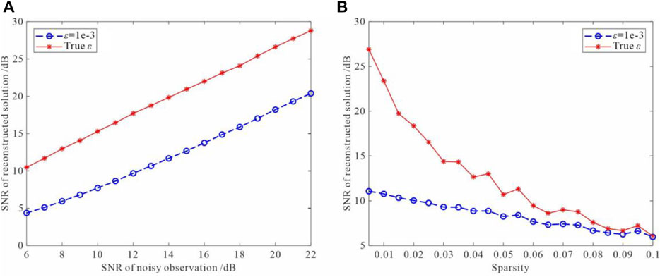
FIGURE 1. Comparison of the performance of different fitting errors. Blue: $\epsilon =1e^{-3}$. Red: ε is the L₂-norm of the noise. (A) SNRs of reconstructed solutions for different ε with a fixed sparsity ($\text{sparsity }=2\text{ \%}$), while varying the observations’ SNRs. (B) Plots of SNRs of reconstructed solutions versus sparsity with the observations’ SNRs are fixed at 10 dB.

FIGURE 2

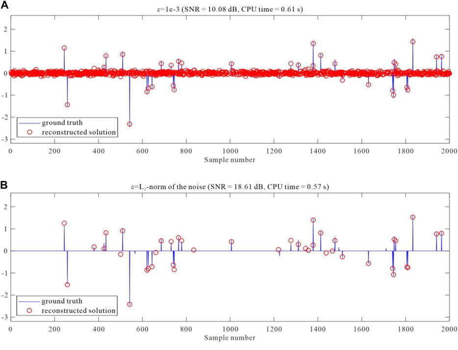
FIGURE 2. Plots of reconstructed solutions for $\epsilon =1e^{-3}$ and ε are the L₂-norm of the noise. Reconstructed solutions (red) are plotted on top of the ground truth (blue). (A) $\epsilon =1e^{-3}$. (B) ε is the L₂-norm of the noise.

3.2 Simulating the Randomly Decimated Data

We first use a five-layer model (Figure 3A) to perform wavefield modeling. The synthetic line has 48 shot gathers, and 48 traces per each shot gather and CMP gather. Source-station and receiver-station spacings are both 50 m. The data are recorded for 1.000 s, with a sample interval of 0.002 s. Figure 3B,C show the reflectivity and seismogram gathers of the first CMP gather. Figure 3D presents the 24th common-offset gather (offset is 50 m). CMP gather is characterized by hyperbolic events, while the common-offset gather consists of flat events, which share approximately equal two-way times. Compared with CMP gather, each trace in common-offset gather shows better similarity and simpler texture structure. This makes it easier to deal with common-offset gather in both the time-space domain and Fourier domain.

FIGURE 3

FIGURE 3. Geologic model and seismic wavefield modeling. (A) Geologic model. (B) first reflectivity CMP gather. (C) first seismogram CMP gather, which is characterized by hyperbolic events. (D) 24th common-offset gather (offset is 50 m), which is characterized by flat events.

The field-recorded seismic data are inevitably perturbed by random noise. Therefore, we add random noise at various levels to the synthetic data to make the SNR of each noisy trace vary within a range of 1–10 dB. The first noisy CMP and the 24th noisy common-offset gathers are shown in Figure 4A,B, respectively. To simulate the irregularly sampled seismic data, we randomly zero out 25% of the receivers and artificially create some gaps to increase the difficulty of the experiments. The incomplete noisy CMP and common-offset gathers are shown in Figure 4C,D, respectively.

FIGURE 4

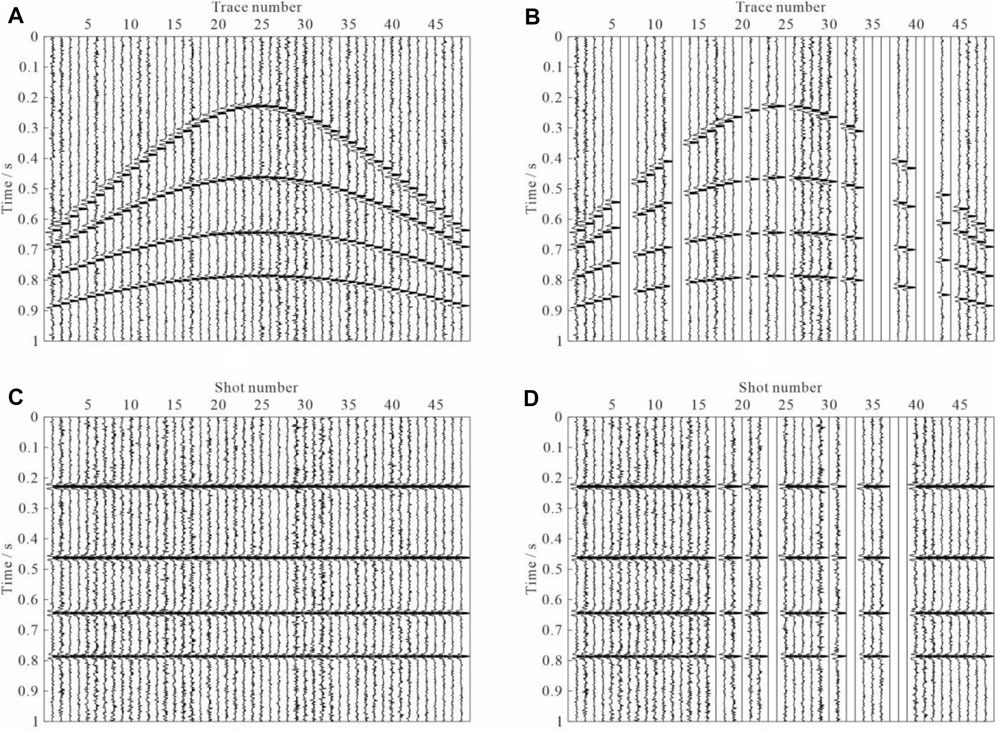
FIGURE 4. Incomplete noisy seismic data. (A) and (B) are complete and incomplete noisy CMP gathers, respectively. (C) and (D) are complete and incomplete noisy common-offset gathers, respectively. 25% of the traces are missing based on the under-sampling strategy.

To inspect the amplitudes of the seismic data at different frequencies and wave-numbers, we perform 2-D Fourier transform on both complete noisy CMP and common-offset gathers to transform them into frequency-wavenumber (f-k) domain, as indicated in Figure 5A,B, respectively. Note that obvious spatial aliasing exists in the f-k spectra for the CMP gather that indicates insufficient sampling of the data along the space axis. However, COG is free from aliasing.

FIGURE 5

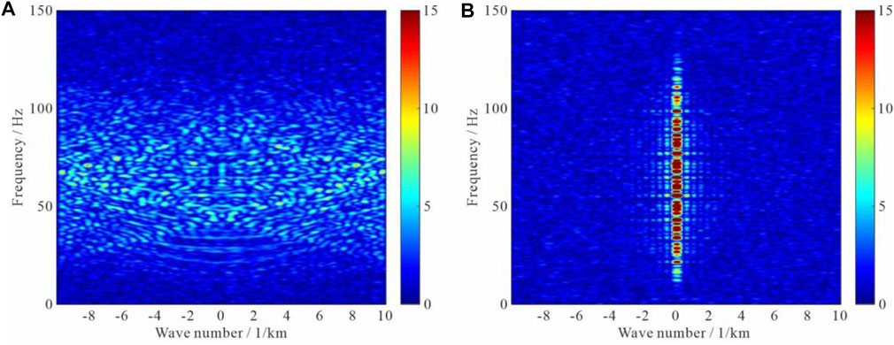
FIGURE 5. f-k spectra for (A) the complete noisy CMP gather and (B) the common-offset gather. Note that apparent spatial aliasing exists in the f-k spectra for the CMP gather. However, COG is free from aliasing.

3.3 Curvelet Transform Operator Tests

Most relevant literature (Zhang et al., 2019; Cao et al., 2020) characterizes the sparse representation of seismic data based on curvelet transform. We use the approved algorithm (curvelet domain approach) to deal with the common-offset and the CMP gathers, separately. The experiment served two purposes: (1) Spatial aliasing has severe effects on the performance of curvelet domain approach in the time-offset domain (common-shot and CMP gathers); (2) Noise estimation and wavefield reconstruction can be done better in the time-midpoint domain (common-offset gather).

Determining an optimal threshold value is an essential first step for sparse representation and the implicit reconstruction and denoising. We first apply the multiple regression theory-based approach to evaluate the noise level both in time-midpoint and time-offset domain, respectively. In implementing this step, we get poor result with CMP gather, as demonstrated in Figure 6A. The estimated L₂-norm of the noise aliasing in each trace is much lower than the actual noise level. This is basically because the multiple regression theory-based method assumes that each trace can be linearly represented by other seismic traces in the gather. CMP gather is characterized by hyperbolic events that have disparate TWT. They share a low correlation between neighboring traces that dissatisfy the multiple regression theory-based method. The procedure is also applied to common-offset gather, and the obtained result is plotted in Figure 6B that indicates that the estimated value is approximately correct.

FIGURE 6

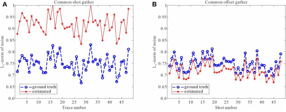
FIGURE 6. Noise estimation by the multiple regression theory-based approach in both (A) the time-offset domain (CMP gather) and (B) the time-midpoint domain (common-offset gather). In all plots, the y-axes represent the L₂-norm of the noise; the x-axes represent the trace number (A) and shot number (B), respectively. Estimated values (red) are plotted on top of the ground truth (blue).

To fill in the gaps and denoise the incomplete noisy data using sparse representation, we use the curvelet transform as “sparse basis” to create matrices A in Eq. 2. The linear relation between the y and m inspires us to consider estimating complete sparse and low-rank coefficient vector ${\mathbf{m}}^{\ast }$ by solving Eq. 4 via the linearized Bregman method. We take ε as the Frobenius norm of noise to balance the fidelity and sparsity. Figure 7A,B are based upon the processing of the CMP gather, and they illustrate reconstructed data (first CMP gather) using the curvelet dictionary and corresponding residual section. It does not seem plausible that the curvelet dictionary is to blame for false artifacts, because the curvelet transform has only a weak ability to anti-aliasing, even though it has proven to have an outstanding ability that enables a nearly optimal representation of seismic data. However, such spatial aliasing can be maximumly remitted in the time-midpoint domain because the common-offset gather is characterized by flat, even approximate horizontal events. The reconstructed results of the first CMP and the 24th common-offset gathers using the time-midpoint domain approach are shown in Figure 7C,E, respectively. Figure 7D,F show the corresponding residuals of the CMP and common-offset gathers, respectively. As expected, the curvelet reconstruction performs much better in the time-midpoint domain than in the time-offset domain. All missing seismic traces are perfectly reconstructed. The defect is that random noise is not well suppressed.

FIGURE 7

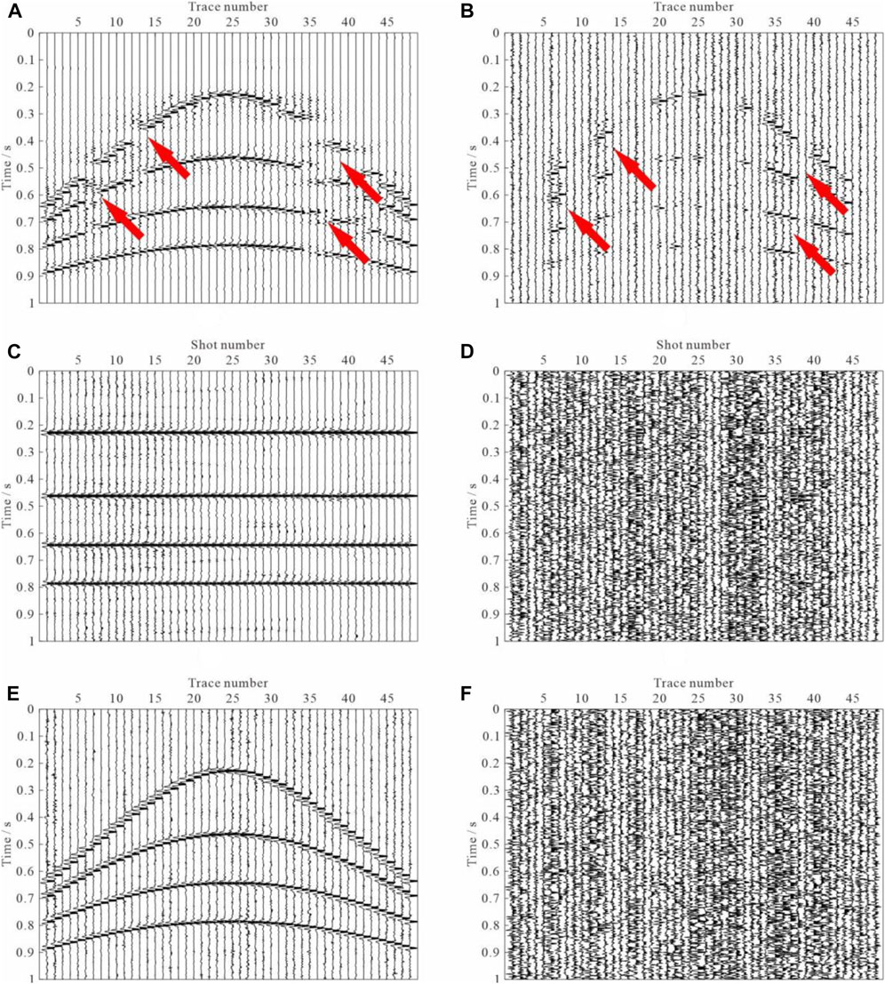
FIGURE 7. Reconstruction results of subsampled data using curvelet interpolation. (A) Recovered CMP gather using linearized Bregman method across CMP gathers in the time-offset domain, and (B) the corresponding residual section. (C) Recovered common-offset gather across offset gathers in the time-midpoint domain, and (D) the corresponding residual image. (E) Recovered CMP gather in the time-midpoint domain, which is the same as in (B). (F) The residual section corresponding to (E).

3.4 Fourier Transform Operator Tests

We next examine whether Fourier transform operator does it as good as the curvelet transform operator. The results from the Fourier transform operator associated with both the time-offset and the time-midpoint domains approaches are plotted in Figure 8A,C, respectively. The corresponding residual images are shown in Figure 8B,D, respectively. There are no apparent differences between curvelet and Fourier transform operators. However, to our surprise, the Fourier transform operator does slightly better than the curvelet transform operator both in the time-offset domain and the time-midpoint domain. The possible reason is that the simulation data used in this experiment are spatially under-sampled. The curvelet transform operator tended to express the local tectonics of the seismic section, and its anti-aliasing ability is weak. The opposite effect is observed for the Fourier transform operator, which points to the ability of the Fourier transform operator to address issues that arose in the field of aliased data. There is no doubt that the computational complexity of the Fourier transform is much lower than the curvelet transform. Therefore, the Fourier transform operator is the best option.

FIGURE 8

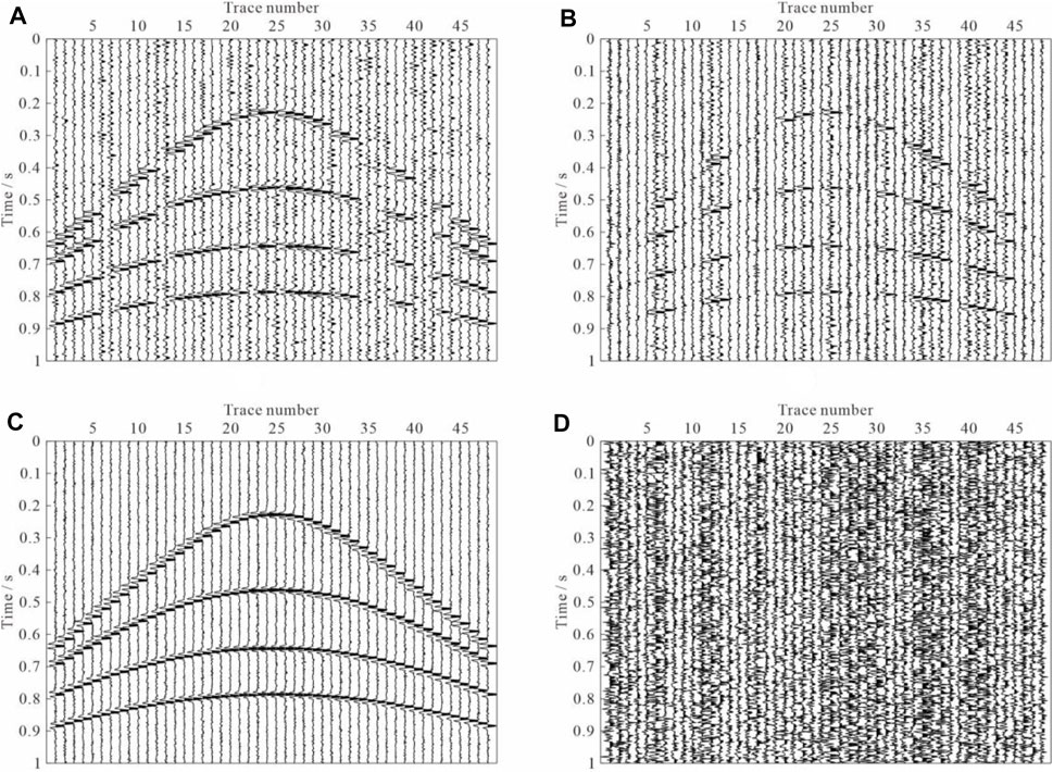
FIGURE 8. Reconstruction results of subsampled data using Fourier interpolation. (A) Recovered CMP gather using linearized Bregman method across CMP gathers in the time-offset domain, and (B) the corresponding residual section. (C) Recovered CMP gather across offset gathers in the time-midpoint domain, and (D) the corresponding residual image.

3.5 Evaluation of the Proposed Sparse and Low-Rank Regularization Approach

We have experimentally verified the superiority of the time-midpoint domain approach and Fourier transform operator in the previous subsection. Naturally, a combination of the two is also appreciated. The assay is performed as described in Subsection 2.1. Figure 9A shows the recovered common-offset gather in the time-midpoint domain, and Figure 9B is the corresponding residual image. Both two objectives of reconstruction and denoising have been achieved. Next, we sort the data into common-shot gathers to obtain the final result shown in Figure 9C, which is very close to the clean synthetic seismogram (Figure 3C). Figure 9D is the corresponding residual image. The proposed approach improves the SNR of seismic data as compared with the previous two experiments.

FIGURE 9

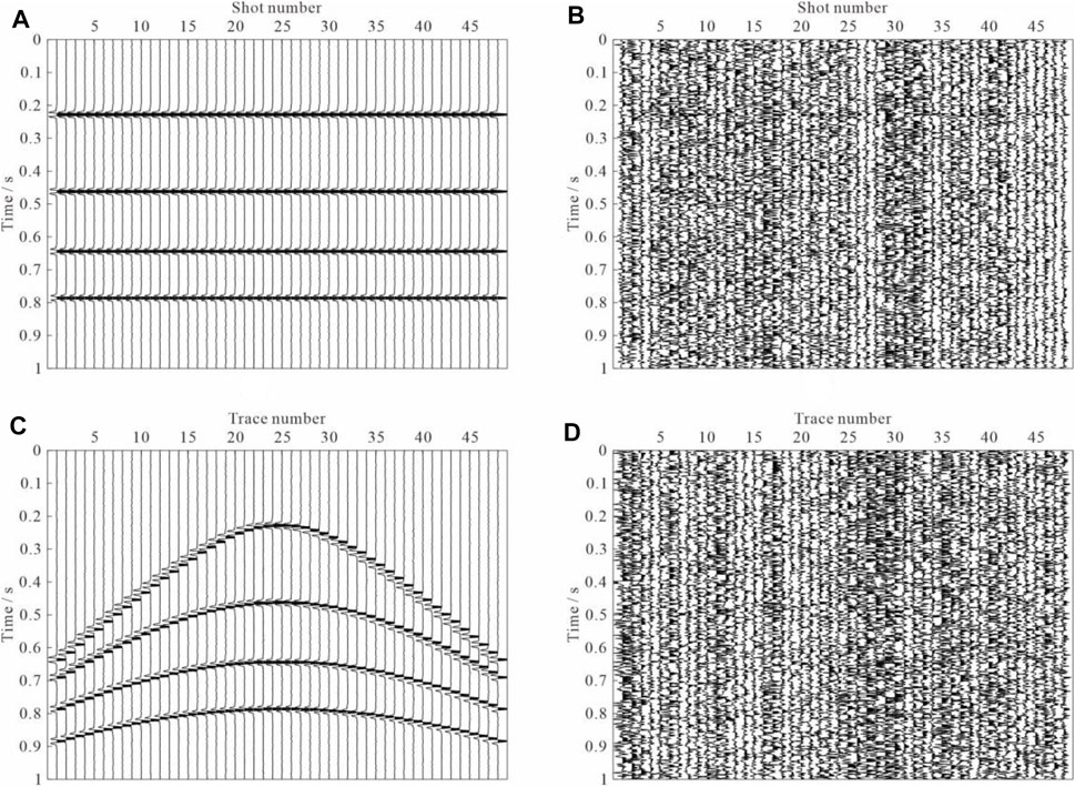
FIGURE 9. Reconstruction results of subsampled data using the proposed method. (A) Recovered common-offset gather across offset gathers in the time-midpoint domain, and (B) the corresponding residual image. We then transform the reconstruction results into CMP gathers to generate (C) and (D). (C) recovered CMP gather. (D) The residual section corresponding to Figure 7C.

To quantitatively compare the reconstruction performance in detail, we plot the noise-free single trace which is a missing trace deleted in the preceding step and the reconstructions with different methods in Figure 10. Figure 10A,E plot the clean and noisy signal (SNR = 4.421 dB), respectively. Results of three independent experiments are all obtained by time-midpoint domain approach, as plotted in Figure 10B–D. Full recovery of the missing trace is perfectly achieved in each of the three experiments. Fourier and curvelet transform operators suppress the random noise and improve the SNR of data to some extent, as plotted in Figure 10B,C. The SNRs of reconstructed traces of the two methods are 6.994 and 7.812 dB, respectively. Comparing the two methods, we can see that the superiority of the proposed method is clear (Figure 10D). SNR of the proposed method is equal to 18.243 dB.

FIGURE 10

FIGURE 10. Single trace comparisons of original data and reconstructed results using the three methods. (A) is the clean 35th trace, which is a missing trace deleted in the preceding step. (B), (C), and (D) Denoised and reconstructed data using curvelet interpolation, Fourier interpolation, and the proposed method, respectively. (E) Noisy synthetic trace with SNR = 4.421 dB. (F), (G), and (H) corresponding differences between (B), (C), and (D) and clean trace (A).

4 Application to Field Seismic Data

In this section, we apply the proposed simultaneous reconstruction and denoising method to a prestack data set. The original raw data consist of 1,001 shot records with 120 channels per shot record. The minimum and maximum offsets are 262 and 3237 m, respectively. Both the source station interval and receiver station interval are 25 m. This study extracts 48 shot gathers from the raw data to ensure that the source station interval is 50 m, exactly twice the original source station interval. Then, each shot gather is down-sampled to reduce the number of channels to 60; that is, the receiver station interval is increased to 50 m. Figure 11A,B show the observed shot gather and common-offset gather, respectively. Intuitively, the shot gather consisted of hyperbolic reflected events and gradient direct and seabed reflection waves. However, the common-offset gather is characterized by much flatter events, which is very well adapted to reconstruction and denoising. Such down-sampling may give rise to spatial aliasing. Figure 12A shows the f-k spectra for the shot record with strong spatial aliasing, as indicated by the solid arrows. As mentioned previously, processing seismic data in the time-shotpoint domain is a simple and efficient strategy. Figure 12B demonstrates the f-k spectra for the common-offset gather shown in Figure 11B, and spatial aliasing is not visible as of the common-shot gather. To simulate the observed incomplete field data, we just take out the columns with missing receivers. 25% of the receivers are deleted randomly in this study. Figure 11C,D show the incomplete shot and common-offset gathers, respectively.

FIGURE 11

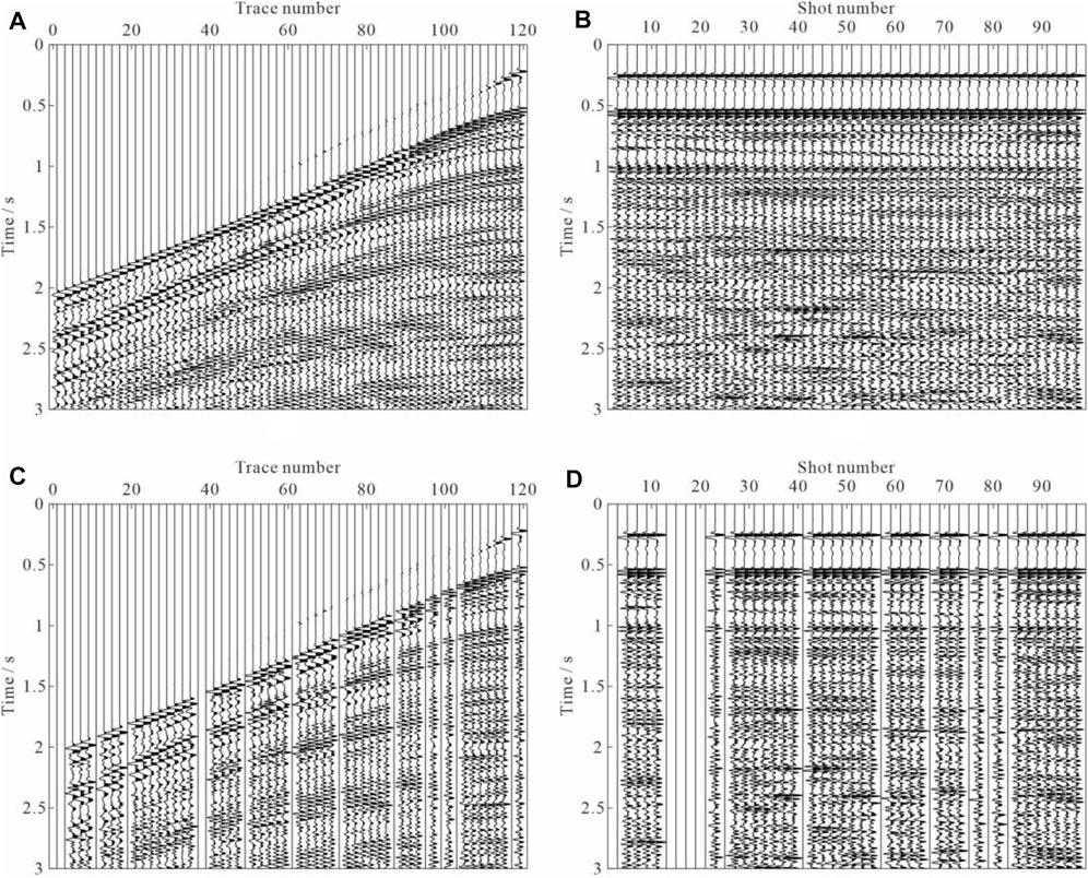
FIGURE 11. Field seismic data. (A) Observed complete common-shot gather, and (B) common-offset gather. Incomplete (C) common-shot gather and (D) common-offset gather, with 30% random missing data.

FIGURE 12

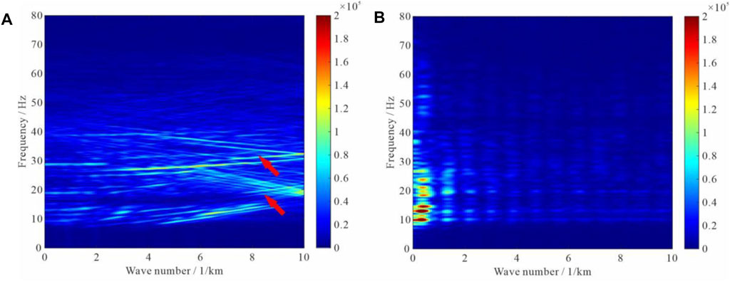
FIGURE 12. f-k spectral analysis for (A) the common-shot gather and (B) the common-offset gather shown in Figure 11A,B.

We perform three shortened versions of the simultaneous reconstruction and denoising experiments on the truncated seismic data, that is, curvelet transform operator, Fourier transform operator, and the proposed sparse and low-rank regularization approach. The complete workflow of each experiment consisted of three flows: (1) transforms the seismic data to the time-shotpoint (common-offset) domain, (2) noise level estimation, and (3) reconstructs the clean and complete seismic section by different methods. The reconstructed common-offset gathers of three different methods are contrasted in Figure 13. The reconstructed result using the curvelet transform operator and the associated difference section are shown in Figure 13A,B, respectively. The narrow gaps are well recovered, while the reconstructed results of the big gaps are not as good as it would be expected (indicated by the arrows in Figure 13A,B). Recovered common-offset gather using Fourier transform operator and the associated difference section are shown in Figure 13C,D, respectively. The missing traces were well recovered, in particular at the big gaps. However, reconstructed data seem to have significant residual noise in the big gap at 0–0.5s. Figure 13E,F demonstrate the interpolated result and the corresponding residuals of the proposed strategy. As can be seen, the recovery is comparable to the Fourier transform operator. A further advantage is that we can obtain much cleaner data that does not contain the artifacts before the first arrivals.

FIGURE 13

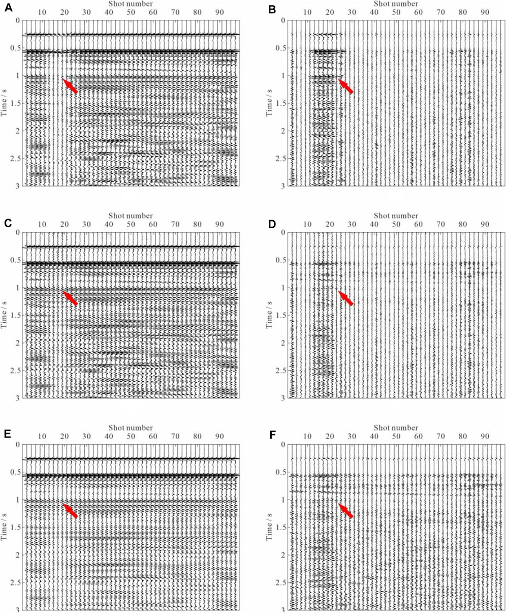
FIGURE 13. Reconstructed common-offset gather. The reconstructed result using (A) the curvelet transform operator and (B) the associated difference section. Result of (C) Fourier transform operator and associated (D) difference section. Result of (E) the proposed sparse and low-rank regularization approach and (F) the associated difference section.

The reconstructed and denoised common-offset gathers are transformed into the common-shot gathers. Figure 14 compares the recovered shot gathers of all the three methods. Figure 14A,C,E indicate the recovered shot gathers of the three different approaches, respectively. Figure 14B,D,F show the corresponding residuals. Similar conclusions can also be obtained based on the comparison of reconstructed results and corresponding residuals of the three methods. The proposed method is more effective in seismic wavefield reconstruction and denoising than the curvelet and Fourier transforms operators. To better compare the details of reconstructed results by the above three methods, we compare the recoveries of a single trace, as plotted in Figure 15. Figure 15A plots the real noisy trace (Trace No. 39 from the noisy shot shown in Figure 11A). Figure 15B–D plot the recovered traces of the three different approaches, respectively. Figure 15E–G correspond to the removed noise associate to each method. These results can be explained as follows. The result of the curvelet transform operator is not very good. The result of the Fourier transform operator is close to the exact solution. However, we should note that the presence of noise before the first arrival (at 0–1.5 s, as indicated by the arrows in Figure 15C,F) is caused by not very good localization of Fourier transform. The proposed method compensates for the defect exactly, and the recovered signal does not contain the evident artifacts and noise. Therefore, the proposed sparse and low-rank regularization approach should be the best choice owing to its effectiveness and fidelity.

FIGURE 14

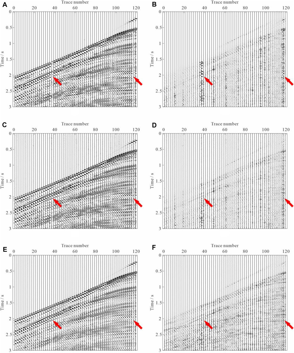
FIGURE 14. Comparison of the reconstructed results of common-offset gathers. The reconstructed result using (A) the curvelet transform operator and (B) associated difference section. Result of (C) the Fourier transform operator and (D) the associated difference section. Result of (E) the proposed sparse and low-rank regularization approach and (F) the associated difference section.

FIGURE 15

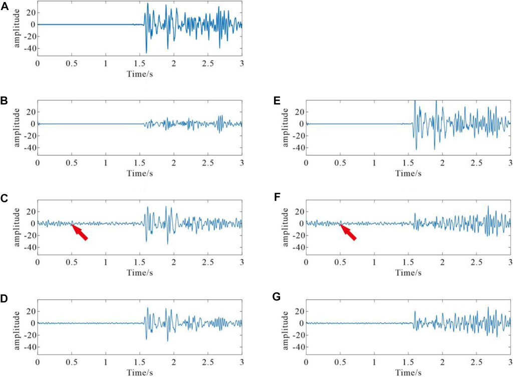
FIGURE 15. Single trace comparisons of original trace and reconstructed traces. (A) Noisy real trace (Trace No. 39 from the noisy shot shown in Figure 11A). Reconstructed results using (B) the curvelet transform operator, (C) the Fourier transform operator, and (D) the proposed sparse and low-rank regularization approach. (E)–(G) Removed noise corresponding to (B)–(D).

5 Discussion

In this work, we present a novel technique for simultaneous reconstruction and denoising of prestack seismic data. To fully exploit the sparse and low-rank nature, we first interpolate the common-offset gather in the 2D Fourier domain, that approach is capable of attenuating random noise to some extent, but new random noise may be introduced. The SVT is then adopted to handle the Fourier coefficient matrix by utilizing the low-rank property, and the residual and generated random noise is washed out. The results shown above demonstrate that it offers a flexible and effective way for both interpolation and denoising.

Curvelet and Fourier transforms are two tools to transform seismic sections into a domain where it has a sparse representation. The computational complexity of the second generation curvelet transform is $O\left(n^2\log n\right)$ for n by n Cartesian arrays, while the complexity of 2D Fourier is $O\left(n^2\right)$ (Candès et al., 2006). had compared the ratio between the running time of the fast discrete curvelet transform (FDCT) and that of the fast Fourier transform (FFT). The ratios of wrapping-based FDCT varied from 6.0793 to 11.2383, and the USFFT-based is 18.2202–28.9579. To compute the curvelet coefficients, we must take on the heavy computational burden. The curvelet transform has only a weak ability to anti-aliasing, even though it has proven to have an outstanding ability in obtaining an essentially optimal representation of seismic data. In Figures 7, 13, and 14, we find that the curvelet transform operator reconstructs single missing-traces accurately. Conversely, the curvelet operator cannot obtain satisfactory results where gaps are existing. In both cases, the Fourier transform operator performs well and reconstructs data accurately.

The proposed method operates in the time-shotpoint domain, characterized by flat, even approximate horizontal events that benefit noise level estimation and seismic wavefield reconstruction. In this work, we choose the multiple regression theory-based approach for noise level estimation. The method assumes that each trace can be linearly represented by other seismic traces in the gather. The common-offset gather rather than the shot gather and CMP gather met the key assumption of the linear mixing scenario. Figure 6 compares the noise estimation results by the multiple regression theory-based approach in both the time-midpoint domain and time-offset domain. The L₂-norm of the estimated noise associated with common-offset gather is much more accurate than that of the CMP. The classical wavefield reconstructions are designed for the case of no spatial aliasing. However, this is an ideal case for both the shot and CMP gathers. Spatial aliasing is encountered frequently in the fieldwork. We find that the steeper the dip, the lower the frequency at which spatial aliasing occurs. Compared to the two gathers, the proposed common-offset gather strategy enjoys its anti-aliasing ability and is bright to handle the under-sampling obstacle. Figures 7–10, 13–15 validate the advantage of the common-offset gather and support our method’s validity.

There are two parameters (regularization parameter α and fitting error ε) in the augmented model (4) that need to be appropriately chosen to ensure that the algorithm converges to the global minimum. L₁-norm regularization is non-differentiable, which is particularly troublesome in numerical optimization. One strategy is to introduce an extra L₂-norm regularization to ensure the objective function is strictly convex. A unique solution could be guaranteed, however, of introducing additional regularization parameter. Fortunately, the relative error is insensitive to α, which only affects the computational efficiency (Yin 2010; Kang et al., 2013). Taking $\alpha =1$ is a logical choice. The fitting error ε denotes the constraint ensures fidelity to the models (1) and (2). However, the importance of parameter ε is often ignored in literature or software packages. $\epsilon =1e^{-3}$ is usually recommended. The parameter ε is essentially an estimate of the noise level of the seismic signal and can be quantified by an upper bound on its norm. To clarify the impacts of the fitting error ε on the augmented model (4), we compare the performance of different fitting errors, that is, $\epsilon =1e^{-3}$ and ε is equal to the L₂-norm of the noise. Output SNRs of reconstructed solutions in terms of SNR and sparsity of noisy observations are plotted in Figure 1A,B, respectively. In Figure 2, reconstructed solutions (red) are plotted on top of the ground truth (blue). It is straightforward to see that output SNR is sensitive to ε, and an appropriate ε consistently increases the precision and accuracy of the solution.

SVT can be achieved in two ways. The first type can be achieved by retaining only the part of the singular values and refers to hard-thresholding. Comparatively, the soft-thresholding is more usually used, which shrinks all the singular values towards zero by a threshold value λ. The difficulty is how to select the proper threshold. A simple and intuitive strategy is an intuitive comparison of the calculated results of various parameters λ. In this article, unbiased risk estimation for the trade-off is obtained with the help of SURE, which is already being applied in MRI and hyperspectral images. The non-parametric simultaneous reconstruction and denoising method is achieved with the automatic estimation of the parameters.

The reconstruction problem (as shown in Eq. 2) involves finding the solution m with the smallest number of non-zero entries that can represent the useful data sparsely and accurately. The accurate identification of the Fourier or curvelet coefficient is crucial for the sparse recovery problem. The discrimination method may help to increase the accuracy of the solutions further. The idea is appealing, as stated in Lindenbaum et al. (2020) and Dong et al. (2020).

6 Conclusion

This article considered the problem of simultaneous interpolation of missing-traces and random noise attenuation. In the approach, we transform the common-offset gather into the 2D Fourier domain and recover the gaps via the linearized Bregman method. SVT attenuates the residual and generated random noise and artifacts. The tandem approach essentially imposes two effective constraints: sparsity and low-rank. In the proposed methodology, we do not assume a single set of hyperparameters but estimate the noise level and the optimal threshold value of SVT by the multiple regression theory and SURE, respectively. These tools allow us to obtain a non-parametric method without person-dependent intervention in the seismic data conditioning. The proposed method handles the common-offset gathers rather than the shot gathers or CMP gathers. Therefore, our approach can provide accurate estimates of the noise level and offers more flexible control on the model, which enjoys its anti-aliasing ability and is bright to handle the highly insufficient seismic gathers. To better handle the spatially aliased data, we use Fourier transform to solve the corresponding sparse representation problem in the time-shotpoint (or time-midpoint) domain. Both synthetic and real seismic data examples confirm the effectiveness of the proposed method for simultaneous wavefield reconstruction and random noise suppression.

Data Availability Statement

The raw data supporting the conclusions of this article will be made available by the authors, without undue reservation.

Author Contributions

LM, ZS, YY, and YW contributed to conception of the study. LM and ZS wrote the first draft of the manuscript. LM, ZS, and YY wrote sections of the manuscript. All authors contributed to manuscript revision, read, and approved the submitted version.

Funding

The financial support from the Key Research and Development Program (Grant No. 21ZDYF2939) of the Science and Technology Department of Sichuan Province, Sichuan Tourism Development Research Center (Grant No. LY22-20), Sichuan Provincial University Key Laboratory of Detection and Application of Space Effect in Southwest Sichuan (Grant No. YBXM202102001), and Leshan Normal University (Grant No. RC2021010).

Conflict of Interest

The authors declare that the research was conducted in the absence of any commercial or financial relationships that could be construed as a potential conflict of interest.

Publisher’s Note

All claims expressed in this article are solely those of the authors and do not necessarily represent those of their affiliated organizations, or those of the publisher, the editors and the reviewers. Any product that may be evaluated in this article, or claim that may be made by its manufacturer, is not guaranteed or endorsed by the publisher.

References

Anvari, R., Kahoo, A. R., Mohammadi, M., Khan, N. A., and Chen, Y. (2019). Seismic Random Noise Attenuation Using Sparse Low-Rank Estimation of the Signal in the Time-Frequency Domain. IEEE J. Sel. Top. Appl. Earth Obs. Remote Sens. 12, 1612–1618. doi:10.1109/JSTARS.2019.2906360

CrossRef Full Text | Google Scholar

Anvari, R., Nazari Siahsar, M. A., Gholtashi, S., Roshandel Kahoo, A., and Mohammadi, M. (2017). Seismic Random Noise Attenuation Using Synchrosqueezed Wavelet Transform and Low-Rank Signal Matrix Approximation. IEEE Trans. Geosci. Remote Sens. 55, 6574–6581. doi:10.1109/TGRS.2017.2730228

CrossRef Full Text | Google Scholar

Batu, O., and Cetin, M. (2011). Parameter Selection in Sparsity-Driven SAR Imaging. IEEE Trans. Aerosp. Electron. Syst. 47, 3040–3050. doi:10.1109/TAES.2011.6034687

CrossRef Full Text | Google Scholar

Becker, S., Bobin, J., and Candès, E. J., (2011). NESTA: A Fast and Accurate First-Order Method for Sparse Recovery. SIAM J. Imaging Sci. 4, 1–39. doi:10.1137/090756855

CrossRef Full Text | Google Scholar

Bekara, M., and Van der Baan, M. (2007). Local Singular Value Decomposition for Signal Enhancement of Seismic Data. Geophysics 72, V59–V65. doi:10.1190/1.2435967

CrossRef Full Text | Google Scholar

Bioucas-Dias, J. M., and Nascimento, J. M. P. (2008). Hyperspectral Subspace Identification. IEEE Trans. Geosci. Remote Sens. 46, 2435–2445. doi:10.1109/TGRS.2008.918089

CrossRef Full Text | Google Scholar

Candès, E., Demanet, L., Donoho, D., and Ying, L. (2006). Fast Discrete Curvelet Transforms. Multiscale Model. Simul. 5, 861–899. doi:10.1137/05064182X

CrossRef Full Text | Google Scholar

Candes, E. J., Sing-Long, C. A., and Trzasko, J. D. (2013). Unbiased Risk Estimates for Singular Value Thresholding and Spectral Estimators. IEEE Trans. Signal Process. 61, 4643–4657. doi:10.1109/TSP.2013.2270464

CrossRef Full Text | Google Scholar

Cao, J., Cai, Z., and Liang, W. (2020). A Novel Thresholding Method for Simultaneous Seismic Data Reconstruction and Denoising. J. Appl. Geophys. 177, 104027. doi:10.1016/j.jappgeo.2020.104027

CrossRef Full Text | Google Scholar

Chang, C.-I., and Du, Q. (2004). Estimation of Number of Spectrally Distinct Signal Sources in Hyperspectral Imagery. IEEE Trans. Geosci. Remote Sens. 42, 608–619. doi:10.1109/TGRS.2003.819189

CrossRef Full Text | Google Scholar

Chen, Y., Chen, X., Wang, Y., and Zu, S. (2019a). The Interpolation of Sparse Geophysical Data. Surv. Geophys. 40, 73–105. doi:10.1007/s10712-018-9501-3

CrossRef Full Text | Google Scholar

Chen, Y., Huang, W., Zhang, D., and Chen, W. (2016a). An Open-Source Matlab Code Package for Improved Rank-Reduction 3D Seismic Data Denoising and Reconstruction. Comput. Geosciences 95, 59–66. doi:10.1016/j.cageo.2016.06.017

CrossRef Full Text | Google Scholar

Chen, Y., and Ma, J. (2014). Random Noise Attenuation Byf-Xempirical-Mode Decomposition Predictive Filtering. Geophysics 79, V81–V91. doi:10.1190/geo2013-0080.1

CrossRef Full Text | Google Scholar

Chen, Y., Peng, Z., Li, M., Yu, F., and Lin, F. (2019b). Seismic Signal Denoising Using Total Generalized Variation with Overlapping Group Sparsity in the Accelerated ADMM Framework. J. Geophys. Eng. 16, 30–51. doi:10.1093/jge/gxy003

CrossRef Full Text | Google Scholar

Chen, Y., Zhang, D., Jin, Z., Chen, X., Zu, S., Huang, W., et al. (2016b). Simultaneous Denoising and Reconstruction of 5-D Seismic Data via Damped Rank-Reduction Method. Geophys. J. Int. 206, 1695–1717. doi:10.1093/gji/ggw230

CrossRef Full Text | Google Scholar

Chen, Y., Zhou, Y., Chen, W., Zu, S., Huang, W., and Zhang, D. (2017). Empirical Low-Rank Approximation for Seismic Noise Attenuation. IEEE Trans. Geosci. Remote Sens. 55, 4696–4711. doi:10.1109/TGRS.2017.2698342

CrossRef Full Text | Google Scholar

Chiu, S. K., and Howell, J. E. (2008). “Attenuation of Coherent Noise Using Localized‐adaptive Eigenimage Filter,” in SEG Technical Program Expanded Abstracts 2008 (Las Vegas: Society of Exploration Geophysicists), 2541–2545. doi:10.1190/1.3063871

CrossRef Full Text | Google Scholar

Deng, L., Yuan, S., and Wang, S. (2017). Sparse Bayesian Learning-Based Seismic Denoise by Using Physical Wavelet as Basis Functions. IEEE Geosci. Remote Sens. Lett. 14, 1993–1997. doi:10.1109/LGRS.2017.2745564

CrossRef Full Text | Google Scholar

Dong, L.-j., Tang, Z., Li, X.-b., Chen, Y.-c., and Xue, J.-c. (2020). Discrimination of Mining Microseismic Events and Blasts Using Convolutional Neural Networks and Original Waveform. J. Cent. South Univ. 27, 3078–3089. doi:10.1007/s11771-020-4530-8

CrossRef Full Text | Google Scholar

Ely, G., Aeron, S., Hao, N., and Kilmer, M. E. (2015). 5D Seismic Data Completion and Denoising Using a Novel Class of Tensor Decompositions. Geophysics 80, V83–V95. doi:10.1190/geo2014-0467.1

CrossRef Full Text | Google Scholar

Gómez, J. L., Velis, D. R., and Sabbione, J. I. (2020). Noise Suppression in 2D and 3D Seismic Data with Data-Driven Sifting Algorithms. Geophysics 85, V1–V10. doi:10.1190/geo2019-0099.1

CrossRef Full Text | Google Scholar

Hansen, P. C. (1992). Analysis of Discrete Ill-Posed Problems by Means of the L-Curve. SIAM Rev. 34, 561–580. doi:10.1137/1034115

CrossRef Full Text | Google Scholar

Hennenfent, G., Fenelon, L., and Herrmann, F. J. (2010). Nonequispaced Curvelet Transform for Seismic Data Reconstruction: A Sparsity-Promoting Approach. Geophysics 75, WB203–WB210. doi:10.1190/1.3494032

CrossRef Full Text | Google Scholar

Jia, Y., and Ma, J. (2017). What Can Machine Learning Do for Seismic Data Processing? an Interpolation Application. Geophysics 82, V163–V177. doi:10.1190/geo2016-0300.1

CrossRef Full Text | Google Scholar

Kang, M., Yun, S., Woo, H., and Kang, M. (2013). Accelerated Bregman Method for Linearly Constrained $$\ell _1$$ - $$\ell _2$$ Minimization. J. Sci. Comput. 56, 515–534. doi:10.1007/s10915-013-9686-z

CrossRef Full Text | Google Scholar

Kreimer, N., and Sacchi, M. D. (2012). A Tensor Higher-Order Singular Value Decomposition for Prestack Seismic Data Noise Reduction and Interpolation. Geophysics 77, V113–V122. doi:10.1190/geo2011-0399.1

CrossRef Full Text | Google Scholar

Kreimer, N., Stanton, A., and Sacchi, M. D. (2013). Tensor Completion Based on Nuclear Norm Minimization for 5D Seismic Data Reconstruction. Geophysics 78, V273–V284. doi:10.1190/geo2013-0022.1

CrossRef Full Text | Google Scholar

Li, F., Xie, R., Song, W.-Z., and Chen, H. (2019). Optimal Seismic Reflectivity Inversion: Data-Driven $\ell_p$ -Loss-$\ell_q$ -Regularization Sparse Regression. IEEE Geosci. Remote Sens. Lett. 16, 806–810. doi:10.1109/LGRS.2018.2881102

PubMed Abstract | CrossRef Full Text | Google Scholar

Lindenbaum, O., Rabin, N., Bregman, Y., and Averbuch, A. (2020). Seismic Event Discrimination Using Deep CCA. IEEE Geosci. Remote Sens. Lett. 17, 1856–1860. doi:10.1109/LGRS.2019.2959554

CrossRef Full Text | Google Scholar

Lu, C., Feng, J., Yan, S., and Lin, Z. (2018). A Unified Alternating Direction Method of Multipliers by Majorization Minimization. IEEE Trans. Pattern Anal. Mach. Intell. 40, 527–541. doi:10.1109/TPAMI.2017.2689021

PubMed Abstract | CrossRef Full Text | Google Scholar

Ma, J. (2013). Three-dimensional Irregular Seismic Data Reconstruction via Low-Rank Matrix Completion. Geophysics 78, V181–V192. doi:10.1190/geo2012-0465.1

CrossRef Full Text | Google Scholar

Mansour, H., Herrmann, F. J., and Yılmaz, Ö. (2013). Improved Wavefield Reconstruction from Randomized Sampling via Weighted One-Norm Minimization. Geophysics 78, V193–V206. doi:10.1190/geo2012-0383.1

CrossRef Full Text | Google Scholar

Nazari Siahsar, M. A., Gholtashi, S., Kahoo, A. R., Marvi, H., and Ahmadifard, A. (2016). Sparse Time-Frequency Representation for Seismic Noise Reduction Using Low-Rank and Sparse Decomposition. Geophysics 81, V117–V124. doi:10.1190/geo2015-0341.1

CrossRef Full Text | Google Scholar

Nazari Siahsar, M. A., Gholtashi, S., Olyaei Torshizi, E., Chen, W., and Chen, Y. (2017). Simultaneous Denoising and Interpolation of 3-D Seismic Data via Damped Data-Driven Optimal Singular Value Shrinkage. IEEE Geosci. Remote Sens. Lett. 14, 1086–1090. doi:10.1109/LGRS.2017.2697942

CrossRef Full Text | Google Scholar

Oliveira, D. A. B., Ferreira, R. S., Silva, R., and Vital Brazil, E. (2018). Interpolating Seismic Data with Conditional Generative Adversarial Networks. IEEE Geosci. Remote Sens. Lett. 15, 1952–1956. doi:10.1109/LGRS.2018.2866199

CrossRef Full Text | Google Scholar

Oropeza, V., and Sacchi, M. (2011). Simultaneous Seismic Data Denoising and Reconstruction via Multichannel Singular Spectrum Analysis. Geophysics 76, V25–V32. doi:10.1190/1.3552706

CrossRef Full Text | Google Scholar

Osher, S., Burger, M., Goldfarb, D., Xu, J., and Yin, W. (2005). An Iterative Regularization Method for Total Variation-Based Image Restoration. Multiscale Model. Simul. 4, 460–489. doi:10.1137/040605412

CrossRef Full Text | Google Scholar

Ramani, S., Zhihao Liu, Z., Rosen, J., Nielsen, J., and Fessler, J. A. (2012). Regularization Parameter Selection for Nonlinear Iterative Image Restoration and MRI Reconstruction Using GCV and SURE-Based Methods. IEEE Trans. Image Process. 21, 3659–3672. doi:10.1109/TIP.2012.2195015

PubMed Abstract | CrossRef Full Text | Google Scholar

Rasti, B., Ulfarsson, M. O., and Sveinsson, J. R. (2015). Hyperspectral Subspace Identification Using SURE. IEEE Geosci. Remote Sens. Lett. 12, 2481–2485. doi:10.1109/LGRS.2015.2485999

CrossRef Full Text | Google Scholar

Roger, R. E., and Arnold, J. F. (1996). Reliably Estimating the Noise in AVIRIS Hyperspectral Images. Int. J. Remote Sens. 17, 1951–1962. doi:10.1080/01431169608948750

CrossRef Full Text | Google Scholar

Ronen, J. (1987). Wave‐equation Trace Interpolation. Geophysics 52, 973–984. doi:10.1190/1.1442366

CrossRef Full Text | Google Scholar

Stein, C. M. (1981). Estimation of the Mean of a Multivariate Normal Distribution. Ann. Stat. 9, 1135–1151. doi:10.1214/aos/1176345632

CrossRef Full Text | Google Scholar

Sternfels, R., Viguier, G., Gondoin, R., and Le Meur, D. (2015). Multidimensional Simultaneous Random Plus Erratic Noise Attenuation and Interpolation for Seismic Data by Joint Low-Rank and Sparse Inversion. Geophysics 80, WD129–WD141. doi:10.1190/geo2015-0066.1

CrossRef Full Text | Google Scholar

van den Berg, E., and Friedlander, M. P. (2009). Probing the Pareto Frontier for Basis Pursuit Solutions. SIAM J. Sci. Comput. 31, 890–912. doi:10.1137/080714488

CrossRef Full Text | Google Scholar

Wang, B., Zhang, N., Lu, W., and Wang, J. (2019). Deep-learning-based Seismic Data Interpolation: A Preliminary Result. Geophysics 84, V11–V20. doi:10.1190/geo2017-0495.1

CrossRef Full Text | Google Scholar

Wang, C., Zhu, Z., Gu, H., Wu, X., and Liu, S. (2019). Hankel Low-Rank Approximation for Seismic Noise Attenuation. IEEE Trans. Geosci. Remote Sens. 57, 561–573. doi:10.1109/TGRS.2018.2858545

CrossRef Full Text | Google Scholar

Wang, Y., Cao, J., and Yang, C. (2011). Recovery of Seismic Wavefields Based on Compressive Sensing by an L1-Norm Constrained Trust Region Method and the Piecewise Random Subsampling. Geophys. J. Int. 187, 199–213. doi:10.1111/j.1365-246X.2011.05130.x

CrossRef Full Text | Google Scholar

Yin, W. (2010). Analysis and Generalizations of the Linearized Bregman Method. SIAM J. Imaging Sci. 3, 856–877. doi:10.1137/090760350

CrossRef Full Text | Google Scholar

Yin, W., Osher, S., Goldfarb, D., and Darbon, J. (2008). Bregman Iterative Algorithms for $\ell_1$-Minimization with Applications to Compressed Sensing. SIAM J. Imaging Sci. 1, 143–168. doi:10.1137/070703983

CrossRef Full Text | Google Scholar

Yuan, S., Wang, S., Luo, C., and Wang, T. (2018). Inversion-based 3-D Seismic Denoising for Exploring Spatial Edges and Spatio-Temporal Signal Redundancy. IEEE Geosci. Remote Sens. Lett. 15, 1682–1686. doi:10.1109/LGRS.2018.2854929

CrossRef Full Text | Google Scholar

Zhang, D., Zhou, Y., Chen, H., Chen, W., Zu, S., and Chen, Y. (2017). Hybrid Rank-Sparsity Constraint Model for Simultaneous Reconstruction and Denoising of 3D Seismic Data. Geophysics 82, V351–V367. doi:10.1190/geo2016-0557.1

CrossRef Full Text | Google Scholar

Zhang, H., Diao, S., Chen, W., Huang, G., Li, H., and Bai, M. (2019). Curvelet Reconstruction of Non‐uniformly Sampled Seismic Data Using the Linearized Bregman Method. Geophys. Prospect. 67, 1201–1218. doi:10.1111/1365-2478.12762

CrossRef Full Text | Google Scholar

Zhou, Y., and Zhang, S. (2017). Robust Noise Attenuation Based on Nuclear Norm Minimization and a Trace Prediction Strategy. J. Appl. Geophys. 147, 52–67. doi:10.1016/j.jappgeo.2017.09.005

CrossRef Full Text | Google Scholar