Responses of Tropical Background State and ENSO Behaviors to Mid-Holocene Forcing Simulated by PMIP3 and PMIP4 Models

The mid-Holocene (MH), a period about 6,000 years ago, provides an opportunity to understand climate change in response to orbital forcing change. Numerical model simulation is an effective tool through which we can study the climate change in the MH, although the climate in the MH can be partly inferred from proxy data. As the Paleoclimate Model Inter-comparison Project phase 4 (PMIP4) recently released the latest simulations for different past climate scenarios, we investigated tropical climate changes, including both the basic state and interannual variability, and tried to find out whether the PMIP phase 3 (PMIP3) and PMIP4 results can be reconciled. Almost all the modelling results show that the inter-hemisphere contrast was enhanced over the tropical Pacific, with warmer and wetter condition on the northern side of the equator and an intensified cross-equatorial flow in the MH than at present, and the annual cycle of the sea-surface temperature (SST) during the MH was reduced. Such background mean state changes arose from the seasonal changes of the solar incident radiation in the MH. In addition to the consistent changes in background mean state changes, some El Niño-Southern Oscillation (ENSO) features, such as the seasonal phase locking feature and periodicity, show consistent changes across the PMIP3 and PMIP4 models, that is, both suites of models exhibit no marked difference in the MH with respect to present-day simulations. In contrast, the modeling results show only agreement on the sign of the ENSO amplitude change (i.e., decrease in the ENSO amplitude in the MH), while the range of reduction varied with model and region. Additionally, the occurrence probability of central Pacific El Niño events increases in the MH, whereas the significance is quite marginal. The modeled changes in the mean state and ENSO serve as a test bed for studying tropical climate system’s response to natural warming, which may provide some insights into understanding climate changes in response to the current anthropogenic warming.

Introduction

In the mid-Holocene (MH) of ∼6,000 years before present, the climate system differed greatly with respect to the present-day climate. It is accepted that the root cause leading to the distinctive MH climate that differed from the present-day climate lies in different orbital parameters in the MH epoch (e.g., Kutzbach and Otto-Bliesner 1982; Kutzbach and Liu 1997; Zheng and Braconnot 2013; Zheng and Yu 2013). Understanding the paleoclimate changes, especially the change in the typical warming period—MH period, has profound meaning.

During the MH, the climate in the Earth system experienced obvious changes. For instance, the insolation at high latitudes in the boreal summer was greater in the MH than in present-day climate; hence, a lot of ice sheets in the Northern Hemisphere (NH) melted (Gong et al., 2015; Gierz et al., 2020). The global monsoon areas and precipitation in the MH were enlarged compared with the present-day based on the evidence from pollen data and model simulations (Kohfeld and Harrison 2000; Jiang et al., 2015). Moreover, the tropical Pacific region also witnessed the orbital-induced climate changes in the MH. Previous studies have shown that the mean state, annual cycle and dominant interannual variability in the tropical Pacific, which is called the El Niño-Southern Oscillation (ENSO), exhibited great changes in response to the orbital forcing alteration in the MH. However, these studies also underscored uncertainty regarding the climate changes in the tropical Pacific region in the MH.

Based on the evidence of fossil corals, Gagan (1998) indicated that parts of the tropics were warmer during the MH than at present-day. In contrast, through measuring δ¹⁸O from proxy data, Koutavas et al. (2006) and Carre et al. (2014) found that the mean sea-surface temperature (SST) during the MH was cooler than that at present-day by about 0.5°^o–3°C. In addition to the mean state, ENSO variability in the MH also had some differences from the present-day. A number of proxy records, such as corals, fossil mollusk shells and ice cores, provide evidence for a weakening ENSO variability during the MH, but the magnitude of this weakening varies in a range of 29–80% (e.g., Tudhope et al., 2001; Koutavas et al., 2006; Koutavas and Joanides 2012; Carre et al., 2014; Emile-Geay et al., 2016). However, an interesting study conducted by Cobb (2013) argued that the fossil coral sequences may be too short to reveal the ENSO activity change for a long period of time, and they even argued that one may not easily obtain the conclusion that a significant reduction of ENSO variability is found in the MH. To summarize, there is no consensus on the magnitude of ENSO variability reduction based on the proxy data. This promotes the paleoclimate community to turn to the model simulation’s help.

During the past several decades, more and more efforts have been devoted to paleoclimate simulations, e.g., the continuous Paleoclimate Model Inter-comparison Project phase (PMIP) projects. They found that the mean SST in the tropical Pacific was around 1°C cooler than the present-day, especially in the tropical Pacific cold tongue region (e.g., Otto-Bliesner 1999; Liu et al., 2000; Otto-Bliesner et al., 2003; Brown et al., 2006), which supports part of the proxy records. Same as proxy records, plenty of modeling studies showed that the ENSO activity in the MH was reduced, but the magnitude of the reduction varied from 5 to 80% (Otto Bliesner et al., 2003; Zheng et al., 2008; Zheng and Yu 2013; Tian et al., 2017; Chen et al., 2019a; Chen et al., 2019b; Brown et al., 2020). Although most modeling studies show an agreement on the sign of ENSO amplitude change during the MH, there are still large uncertainty regarding the specific magnitude of ENSO amplitude change among these modelling studies.

Recently, the PMIP phase 4 (hereafter PMIP4) simulation results were released (Kageyama et al., 2018), it is necessary to find out whether the PMIP phase 3 (hereafter PMIP3) and PMIP4 results can be reconciled. Here we focused on the mean state, annual cycle and ENSO activity reconstructed by the PMIP4 models over the tropical Pacific during the MH. The simulations of the PMIP3 models were used to be compared with those of the PMIP4 models, and the discrepancies of simulation results between PMIP3 and PMIP4 models were analyzed. The data used in this study is introduced in Section 2. The simulation results of mean state and annual cycle are shown in Section 3, and the ENSO variability is examined in Section 4. We summarize this study in Section 5.

Data

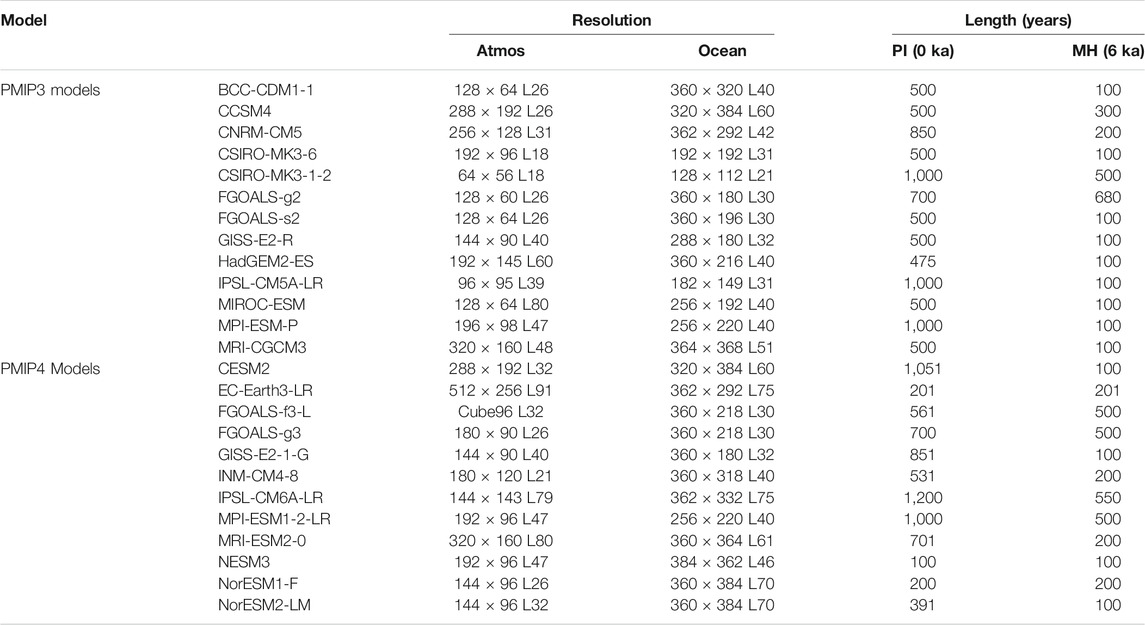
The simulation for the MH climate period is one of the important experiments in the PMIP, which is also part of Coupled Model Intercomparison Project (CMIP). According to the data ability, 13 PMIP3 models and 12 PMIP4 models were used in this study. The basic information of the 25 models are presented in Table 1, and the boundary conditions for the MH simulation in both PMIP3 and PMIP4 are shown in Table 2. The primary difference between the PMIP3 and the PMIP4 experiments boundary conditions lies in greenhouse gases (GHG) concentration, and the other boundary conditions such as ice-sheets, aerosols and solar constant are identical. The variables used in this study include SST, precipitation, surface wind stress, sea water potential temperature and top of the atmosphere incident shortwave radiation. Due to the different model horizontal resolutions, all data were interpolated onto a regular 1° × 1 ° (latitude x longitude) grid.

TABLE 1

TABLE 1. Information describing the model resolutions and simulation length.

TABLE 2

TABLE 2. Model boundary conditions.

Tropical Background State

Mean States

The tropical climate states of SST and wind stress during the PI and MH of 13 PMIP3 models and 12 PMIP4 models and their differences in terms of multi-model ensemble mean (MME) are shown in Figure 1. In the present-day climate simulations (Figures 1A,D) and MH simulations (Figures 1B,E), both PMIP3 and PMIP4 models show similar large-scale distribution features, including the cold tongue in the eastern equatorial Pacific, the warm pool in the western Pacific, and the surface winds converging toward the warm surface temperature region. In general, the trade wind and mean SST appear approximately symmetric with respect to the equator over the western tropical Pacific, while the mean SST exhibits asymmetric distribution with respect to the equator over the eastern tropical Pacific (i.e., warm SST in the northeastern part but cold SST in the southeastern part), matching the cross-equatorial southerly over the eastern Pacific, especially the southerly near the coast of Peru. The difference maps (Figures 1C,F) show the mean SST cooling to various extent over the entire tropical Pacific in the MH compared to that in the PI. In the MMEs of both PMIP3 and PMIP4 models, the magnitude of the cooling in the tropical Pacific reached about 0.1°–0.6°C in the MH. In general, the decrease in the mean SST in the MH is greater in the western equatorial Pacific than in the eastern equatorial Pacific, indicating a slightly westward extension of the cold tongue. The obvious feature from the difference maps (Figures 1C,F) lies in the inter-hemisphere contrast, that is, the mean SST cooling over the tropical Pacific is more obvious in the Southern Hemisphere (SH) than in the NH, consistent with the cross-equatorial southerly. Previous studies (e.g., Luan et al., 2012; Zhao and Harrison 2012) suggested that such inter-hemisphere contrast may result from the strengthened monsoon precipitation in the NH and weakened monsoon precipitation in the SH, which fundamentally stems from orbital forcing change, that is, the enhanced summer insolation in the NH and reduced summer insolation in the SH. It is noted that such inter-hemisphere contrast is slightly stronger in the MME of the PMIP4 models than of the PMP3 models.

FIGURE 1

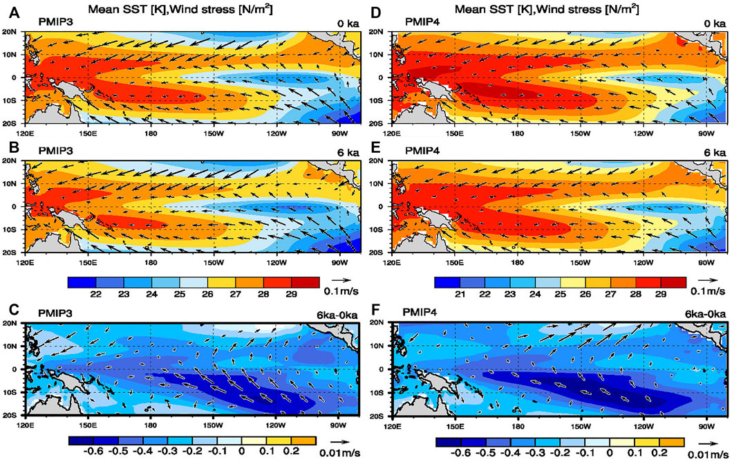
FIGURE 1. Plots for MME of mean SST and surface wind stress derived from PMIP3 (left column) and PMIP4 (right column) models. (A) and (D) are PI simulations; (B) and (E) are MH simulations; and (C) and (F) are their differences (MH minus PI). Shading and vector in (C) and (F) indicate the difference between MH and PI is significant at the 95% level by Student’s t-test.

Figure 2 shows the spatial distribution of mean precipitation in the PI and MH simulations, as well as their differences. The simulated mean precipitation in the PI simulations resembles that in the observation (not shown), except for the excessive eastward extension of the South Pacific convergence zone (SPCZ), which is associated with the notorious double-intertropical convergence zone (ITCZ) bias—a prevalent bias in coupled models. It is worth mentioning that such double-ITCZ bias is slightly alleviated in the PI simulations of the PMIP4 models compared to the counterpart in the PMIP3. Next, we analyze the difference of tropical mean precipitation in the MH with respect to the PI. As shown in Figures 2C,F, the difference in mean precipitation in the MH also exhibits marked inter-hemisphere contrast, that is, more precipitation in the NH than in the SH. Such asymmetric mean precipitation difference distribution is consistent with the aforementioned inter-hemisphere contrast of the mean SST and surface wind. Again, the magnitude of the difference in the mean precipitation is slightly larger in the PMIP4 than in the PMIP3.

FIGURE 2

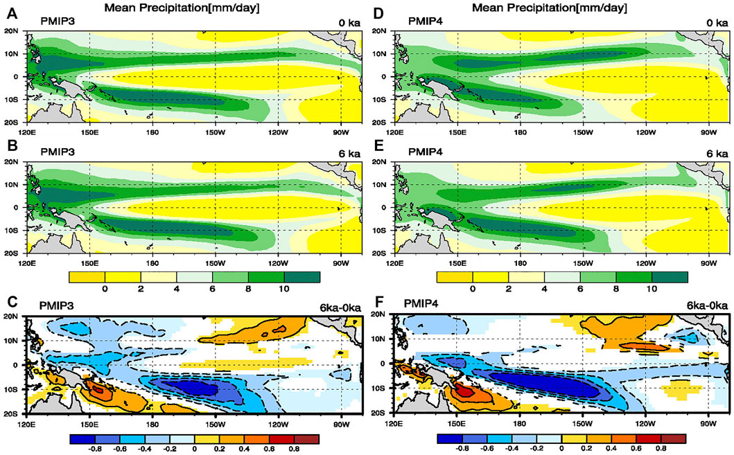
FIGURE 2. Plots for MME of mean precipitation derived from PMIP3 (left column) and PMIP4 (right column) models. (A) and (D) are PI simulations; (B) and (E) are MH simulations; and (C) and (F) are their differences (MH minus PI). Shading and vector in (C) and (F) indicate the difference between MH and PI is significant at the 95% level by Student's t-test.

Figure 3 shows the equatorial profile of the mean thermocline depth for the MME results from the PI and MH simulations. We can see that the difference in the equatorial mean thermocline during the MH and PI is negligible; this feature is also true for the individual models (not shown). This may be due to the fact that surface flow changes are insignificant for the zonal wind at the equator during the MH, although the southerly wind difference is obvious. The insignificant difference in surface zonal wind may be responsible for the similar equatorial mean thermocline profiles in the two periods.

FIGURE 3

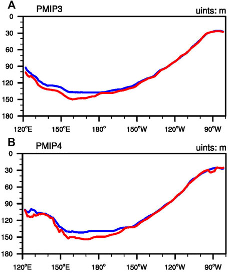
FIGURE 3. Plots for MME of mean thermocline depth alone the equator (averaged between 5^oS and 5^oN) derived from (A) PMIP3 and (B) PMIP4 models. The depth of the mean thermocline is calculated from the location at the maximum vertical gradient of the mean temperature. Blue and red lines indicate PI and MH simulations, respectively.

Annual Cycle

In this subsection, we examine the annual cycle of SST in the equatorial (5^oS–5^oN) Pacific derived from the MMEs of the PMIP3 and PMIP4 models. The annual cycle is characterized by the climatological monthly average after removing the long-term annual mean. As shown in Figures 4A,D, the PI simulations in both PMIP3 and PMIP4 models show an obvious annual cycle of SST in the eastern equatorial Pacific, close to that in the observation (not shown). When comparing the annual cycle result in the PI simulations with the MH simulations, we find that the annual cycle in the eastern equatorial Pacific is weaker in the MH simulations (Figures 4B,E). Additionally, the peak interval time of the annual cycle in the MH shows a slight difference from that in the PI simulations, that is, the annual cycle of SST in the eastern Pacific reached its positive peak in april and negative peak in August in the PI simulations, whereas the positive peak was slightly shifted toward May and the negative peak, shifted toward July in the MH simulations.

FIGURE 4

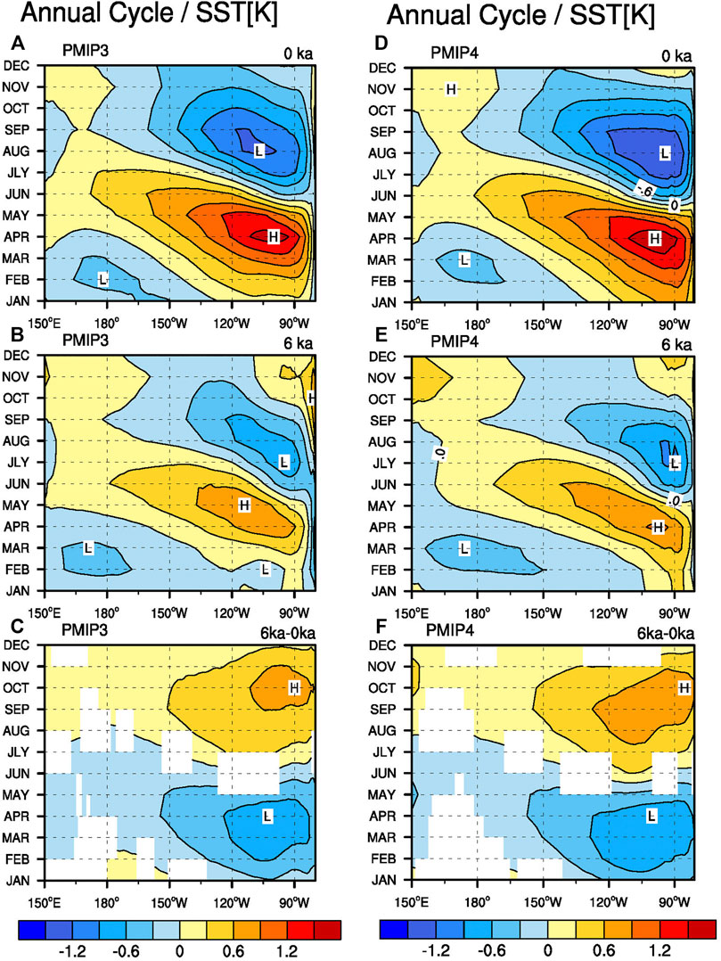
FIGURE 4. Plots for MME of SST annual cycle over the equatorial Pacific (averaged between 5^oS and 5^oN) derived from PMIP3 (left column) and PMIP4 (right column) models. (A) and (D) are PI simulations; (B) and (E) are MH simulations; and (C) and (F) are their differences (MH minus PI). Letters H and L represent the positive and negative centers, respectively. Shading in (C) and (F) indicate the difference between MH and PI is significant at the 95% level by Student’s t-test.

Two factors are responsible for the obvious weakening in the annual cycle of SST in the MH. Following Xie (1994) and An and Choi (2013); An and Choi (2014), the physical reason for the reduced annual cycle amplitude can be explained by the following equation that describes the annual cycle amplitude of SST,

$\frac{\partial \langle ML{T}_{AC}^2\rangle }{\partial t}=-\left({\overline{u}}_0-c\right)\frac{\partial \langle ML{T}_{AC}^2\rangle }{\partial x}+\frac{4}{\rho C_{p}h}\langle SW\cdot ML{T}_{AC}\rangle -\left(1+\beta \right)\frac{4\overline{LH}}{\rho C_{p}h}\frac{\overline{v}}{{\left|\overline{u}\right|}^2}\langle v_{AC}\cdot ML{T}_{AC}\rangle -2\epsilon \langle ML{T}_{AC}^2\rangle (1)$

where MLT indicates mixed layer temperature, subscript AC indicates the annual cycle after removing the annual mean, c is the phase speed associated with air-sea interaction, h represents mixed layer depth, ${\overline{u}}_0$ indicates mixed layer-averaged mean zonal current, and $\beta$ denotes the vertical mixing effect on the latent heat flux. $\overline{u}\text{and}\overline{v}$ indicate the mean zonal and meridional winds, respectively. $\epsilon$ denotes the Newtonian cooling coefficient. LH and SW are the mean latent heat flux and the perturbed solar radiation, respectively. It is worth noting that the amplitude of SST annual cycle is directly defined as the difference between the maximum and the minimum (e.g., Chen and Jin 2018), which means that the amplitude of SST annual cycle is closely related to the seasonal evolution of the corresponding SST tendency. Considering that the positive SST tendency will be offset by the negative SST tendency in a calendar year, a mathematical treatment is conducted through multiplying both sides of the original mixed layer temperature (MLT) tendency equation by $ML{T}_{AC}$. In this way, we obtained Equation 1 and the term $\frac{\partial \langle ML{T}_{AC}^2\rangle }{\partial t}$ in the left-hand side of Equation 1 is proportional to the overall SST (or MLT) tendency that determines the annual cycle magnitude. Previous studies (e.g., An and Choi 2013, 2014) pointed out that the annual cycle amplitude of SST is largely determined by the second and third terms on the right-hand side of the equation, that is, by the factors associated with the solar radiation and latent heat flux.

The change in the annual cycle of SST during the MH can be traced back to the orbital parameter change (Clement et al., 2000; Braconnot et al., 2012a), that is, the insolation at the top of the atmosphere, which varies between spring and fall, as a result of the orbital-induced alteration during the MH (Berger 1978). As shown in Figure 5, the incoming solar radiation is less in early calendar months (especially February) but more in the boreal summer (especially August) in the equatorial region. According to the second term on the right-hand side of Eq. 1, such change in the incoming solar radiation can cause a weakened annual cycle of SST in the MH. Consequently, the annual cycle of SST shows a decrease in the MH simulations compared to that in the pI. Moreover, the slightly intensified cross-equatorial wind may lead to a slight deepening in the ocean mixed layer (not shown) due to the strengthened stirring effect. The second and third terms on the right-hand side of Eq. 1 indicate that the annual cycle amplitude is inversely proportional to the mixed layer depth h; thus, the slightly deepened mixed layer can cause the increase in the thermal inertia and the reduction of the annual cycle amplitude of SST.

FIGURE 5

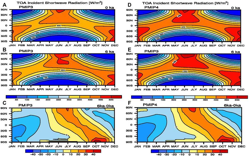
FIGURE 5. MME of mean insolation at the top of the atmosphere over the tropical Pacific (averaged between 120^oE and 160^oE) from PMIP3 (left column) and PMIP4 (right column) models. (A) and (D) are PI simulations; (C) and (B) are MH simulations; and (C) and (E) are their difference (MH minus PI).

Note that the shading in Figures 1C,F, Figures 2C,F, Figures 4C,F indicates the difference between the MH and PI simulations is significant based on Student’s t-test. To summarize, the modelled tropical Pacific mean states during the MH show an agreement across the PMIP3 and PMIP4 models, including the mean SST cooling in the tropical Pacific with severely cooling in the SH, mean precipitation decrease in the SH but slight increase in the NH, insignificant difference in the mean thermocline depth in the equatorial Pacific, and remarkable weakening in the annual cycle of SST in the eastern equatorial Pacific.

El Nino-Southern Oscillation

In this section, we focus on whether there were some obvious differences in the dominant interannual mode of the ENSO during the MH. The ENSO activity is commonly described by the standard deviation (STD) of SST anomalies. Figure 6 shows the STDs of monthly SST anomalies averaged in the central-eastern equatorial Pacific in each of the PMIP3 and PMIP4 models. First, the majority of the models show that the mature phase of ENSO is phase-locked to the boreal winter (November–January) in the PI simulations, although a few models fail to show such phase-locking feature. When comparing the seasonal phase-locking feature between the PI and MH simulations, we can clearly see that there are nearly no differences in ENSO phase-locking feature.

FIGURE 6

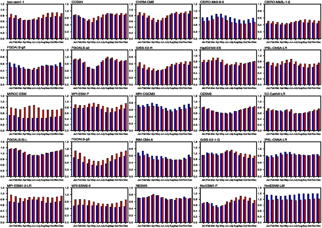
FIGURE 6. Monthly STD of SST anomalies in the equatorial Pacific (160^oE–90^oW, 5^oS–5^oN) for the PI (blue bar) and MH (red bar) simulations from PMIP3 and PMIP4 models. Unit is K.

Figure 7 shows the spatial distribution of the STD of SST anomalies averaged over the boreal winter (November–January) for the MMEs of PMIP3 and PMIP4 models. The difference plots between MH and PI simulations (Figures 7C,F) show an obvious decrease in the interannual variation of SST anomalies over the central-eastern equatorial Pacific, indicating a reduced ENSO activities during the MH. Additionally, the extent of the reduction is more obvious in the PMIP4 MME than in the PMIP3 MME. Note that in both PMIP3 and PMIP4 models, the stippling denotes that the majority of the models (i.e., exceeding two thirds) show an agreement with the change sign, indicating the majority show suppressed ENSO variability.

FIGURE 7

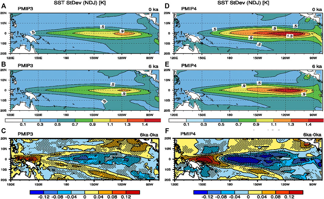
FIGURE 7. Standard deviation of SST anomalies in boreal winter (November–January) obtained from PMIP3 (left column) and PMIP4 (right column) models. (A) and (D) are PI simulations; (B) and (E) are MH simulations; and (C) and (F) are their differences. Stippling in (C) and (F) indicates the model consistency exceeds two thirds of the total model’s count.

To show the spread of ENSO variability changes across the models, we plot the box and whisker chart. As shown in Figure 8, there is large uncertainty regarding the changes in ENSO-related SST anomalies during the MH. For one thing, the spread among the models is somewhat large. Moreover, the magnitude of reduction in MME is small, although the overall variation of SST anomalies shows decreases in different regions, including the Niño3, Niño4, and Niño3.4 regions. For instance, the STDs of the Niño3.4 index are 0.86 and 1.15 for the MMEs of PMIP3 and PMIP4 PI simulations, respectively; and the counterpart in the MH simulations are only 0.81 and 1.05 for the MMEs of the PMIP3 and PMIP4, showing a reduction of about 5.8% and 8.7%, respectively. Recall the relatively large spread among the models, such minor reduction may cause a loss of certainty regarding the modeled changes in ENSO variability. For the Niño1+2 region, a core region for the ENSO, the difference in the variation of SST anomalies between the MH and PI is negligible (Figure 8D). Since the reductions in the variation of SST anomalies are somewhat small in the MMEs of the PMIP3 and PMIP4 models, we use Figure 9 to clearly show these small changes. Nearly all the scatters that represent the STDs of the SST anomalies over the Niño1+2 region for the PI and MH simulations are located along the diagonal line (Figure 9A), indicating little change regarding the variation of SST anomalies in the Niño1+2 region. For the regions to the west (Niño3, Niño3.4, and Niño4), the number of the models that show weaker STDs of SST anomalies in the MH than in the PI increases. Such increase may be partly due to the fact that most of the coupled models exhibit westward shifting bias in simulating ENSO-related SST anomalies (Fang and Xie 2020; Ge and Chen 2020; Zhang et al., 2020). As a result, the changes in the Niño4 and Niño3 regions are more dominant.

FIGURE 8

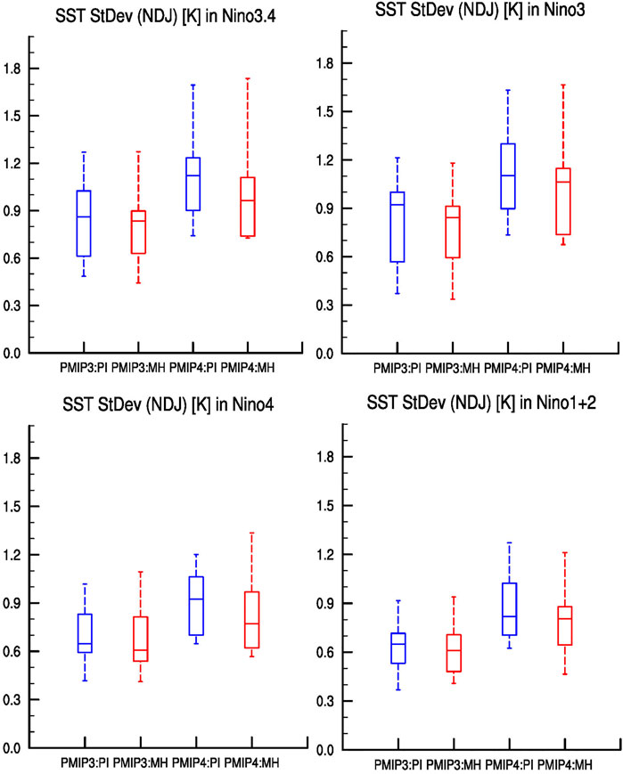
FIGURE 8. Boxplots for standard deviation of various ENSO indices for PMIP3 and PMIP4 models. Blue boxes indicate the PI simulations, and red boxes indicate the MH simulations. The upper and lower bounds of each box represent 25th and 75th percentiles, respectively; the solid line in the middle of each box is the median; and whiskers are the maximum or minimum, respectively. Definitions for each area: Niño1+2 (90^o–80^oW, 0^o–10^oS). Niño3 (150^o–90^oW, 5^oS–5^oN), Niño3.4 (170^o–120^oW, 5^oS–5^oN), and Niño4 (160^oE–150^oW, 5^oS–5^oN).

FIGURE 9

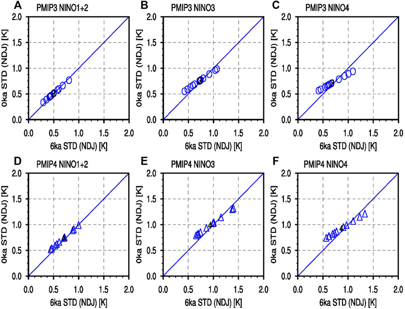
FIGURE 9. Scatter plots for the STD of the ENSO indices in boreal winter (November–January) derived from PMIP3 and PMIP4 models. The MMEs of PMIP3 and PMIP4 models are marked by 3 and 4, respectively. (A) and (D) for Niño1+2 (90°–80°W, 0°–10°S) indices, (B) and (E) for Niño3 (150°–90°W, 5°S–5°N) indices, and (C) and (F) for Niño4 (160°E–150°W, 5°S–5°N) indices.

To summarize the changes of ENSO-related SST anomalies, we present the violin plots for all the PMIP3 and PMIP4 models. Figure 10 shows the probability density of each relevant index. The results are consistent with the aforementioned results building on the PMIP3 or PMIP4 models only, that is, the ENSO-related SST anomalies in the Niño4, Niño3.4, and Niño3 regions exhibit a weakening to some extent in the MH compared to the PI, where the uncertainty remains large.

FIGURE 10

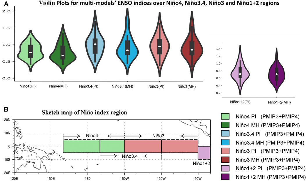
FIGURE 10. Violin plots (A) for STD of winter (November–January) El Niño indices based on PMIP3 and PMIP4 models during the PI (light color) and MH (dark color). Unit is K. The black outline is the probability density of each index’s STD. The solid black boxes are the interquartile range, and the white circle in the black box is the median value. (B) is the schematic plot of ENSO index distribution region.

So far, various mechanisms have been put forward to account for the suppressed ENSO amplitude in the MH. For instance, Clement et al. (2000) indicated the reduced ENSO variance is regarded as a response to the orbital-induced change of the tropical annual cycle. Liu et al. (2000) suggested the deepened mean equatorial thermocline and the strengthened Asian summer monsoon may lead the suppression of ENSO intensity in MH. Moreover, Zheng et al. (2008) pointed out that the reduction of ENSO intensity is interpreted as the influence of strengthened easterly trade wind in tropic Pacific. Chen et al. (2019a); Chen et al. (2019b) suggested that the changes in the mean Pacific subtropical cell (STC) is the key factor responsible for the reduced ENSO intensity in the MH. In a word, the real physical reason for the inhibition of ENSO activity in the MH period is complex, which still needs some more in-depth investigation in the future.

Next, we examine whether there is any change in terms of ENSO periodicity. Figure 11 suggests almost no change regarding the spectrum, for either PMIP3 or PMIP4 MME. Such results indicate that the ENSO period is not sensitive to the orbital forcing change in the MH, at least in the current climate models.

FIGURE 11

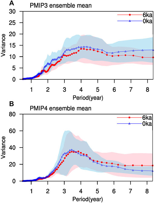
FIGURE 11. MME of power spectrum derived from (A) PMIP3 and (B) PMIP4 models. Blue and red colors indicate the PI and MH simulations, respectively.

In addition to ENSO amplitude and periodicity, we also investigate the change in ENSO diversity in response to the orbital forcing. Several studies uncovered a new flavor of El Niño events in recent years, which is characterized by warm SST anomalies in the central Pacific (CP) and usually called the CP El Niño, El Niño Modoki, warm pool El Niño, or dateline El Niño (Larkin and Harrison 2005; Ashok et al., 2007; Kug et al., 2009; Yu and Kao 2009; Chen et al., 2018). Based on the criteria proposed by Kug et al. (2009), we first compare the SST anomalies in the boreal winter averaged in the Niño3 region with that in the Niño4 region for certain El Niño event, and then label this event as the eastern Pacific (EP) El Niño (CP El Niño), if the Niño3 index is greater (less) than the Niño4 index. Figure 12 shows the ratio of the CP El Niño number to the EP El Niño number for each model and its corresponding MME. Clearly, a divergent performance in simulating the change of the ratio exist across the models. Half of the PMIP3 models (six out of the 13 models) show the ratio of the incidence of CP El Niño events to the EP El Niño events in the MH outstrips the that in the PI, and five among them exhibit a significant increase in the occurrence of CP El Niño during the MH at the 95% confidence level. For the PMIP4 models, eight out of the 12 models record more incidence of CP El Niño events during the MH, and five among them have enhanced ratios exceeding the 95% confidence level. Then, we obtain the MMEs for the PMIP3 and PMIP4 models (the rightmost columns of Figures 12A,B). The increase of CP El Niño events during the MH is minor and insignificant for the PMIP4 MME. Although the increase of CP El Niño events during the MH is relatively large for the PMIP3 MME, it is also not statistically significant at the 95% significant level. Overall, the model results show a larger occurrence of CP El Niño in the MH than in the PI, though the significance is quite marginal.

FIGURE 12

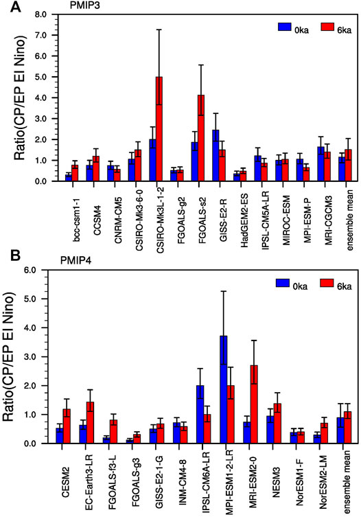
FIGURE 12. Rates of different types of El Niño obtained from (A) PMIP3 and (B) PMIP4 models. Blue and red bars represent PI and MH simulations, respectively. The error bars represent the upper and lower limits of varying range in the occurrence ratio at the 95% confidence level by using the bootstrap method.

Summary

Increasing attention has been given to understand tropical climate change, especially in terms of ENSO behaviors, in response to global warming; however, some puzzles remain (e.g., Collins et al., 2010; Chen et al., 2015; Chen et al., 2017). One way to gain confidence in future projections is to evaluate current models’ performances in simulating past climate changes (Braconnot et al., 2012a; Braconnot et al., 2012b), because some proxy datasets can be used as reference. Here, we investigated the response of tropical Pacific climate to the orbital forcing in the MH, an epoch about 6,000 years ago, by analyzing model results. Although the climate in MH can be partly inferred from proxy data, model simulation is an effective tool through which we can study the climate change in the MH.

Using recently released PMIP4 outputs along with PMIP3 archives, we examined tropical climate changes, including both basic state and interannual variability; we then attempted to find out whether there is any aspect that can be reconciled for the PMIP3 and PMIP4 model results. The main conclusions are summarized here.

1) All the PMIP3 and PMIP4 models show the enhancement of the inter-hemisphere contrast over the tropical Pacific, including the warmer and wetter condition north of the equator and an intensified cross-equatorial flow in the MH than at present. This difference can be attributed to the change in the orbital forcing, or more straightforwardly, the change in the solar incident radiation.

2) Most models show a weakening in the annual cycle of SST during the MH. The relevant air-sea processes may be more complicated, although such background mean state changes can also be linked to the orbital forcing change in the MH. Specifically, the weakened annual cycle amplitude of SST primarily arises from the seasonal change in the incoming solar radiation during the MH, and the slight shoaling in the mixed layer depth plays a secondary role.

3) The majority of the PMIP3 and PMIP4 models show that ENSO amplitude was suppressed during the MH, while the range of reduction varies with model and region. When synthesizing the overall probability distribution of the changes in ENSO indices, we found that the results remain large uncertainty, which varies with space and pattern. Additionally, the occurrence probability of CP El Niño events increased in the MH, whereas the significance is quite marginal. Interestingly, the other ENSO behaviors, such as the seasonal phase-locking feature and periodicity, exhibit no obvious differences between the MH and PI simulations.

Data Availability Statement

Publicly available datasets were analyzed in this study. This data can be found here: https://esgf-node.llnl.gov/search/cmip6/, https://esgf-node.llnl.gov/search/cmip5/.

Author Contributions

M-ES contributed to data analysis and paper writing, LC designed this study and paper writing.

Funding

This work was jointly supported by the National Key Research and Development Program on Monitoring, Early Warning and Prevention of Major Natural Disaster (2019YFC1510004), the Natural Science Foundation of Jiangsu (BK20190781), the National Natural Science Foundation of China (No. 42005020), the General Program of Natural Science Foundation of Jiangsu Higher Education Institutions (19KJB170019), and the Open Fund of State Key Laboratory of Loess and Quaternary Geology (SKLLQG 1802).

Conflict of Interest

The authors declare that the research was conducted in the absence of any commercial or financial relationships that could be construed as a potential conflict of interest.

Publisher’s Note

All claims expressed in this article are solely those of the authors and do not necessarily represent those of their affiliated organizations, or those of the publisher, the editors, and the reviewers. Any product that may be evaluated in this article, or claim that may be made by its manufacturer, is not guaranteed or endorsed by the publisher.

References

An, S.-I., and Choi, J. (2013). Inverse Relationship between the Equatorial Eastern Pacific Annual-Cycle and ENSO Amplitudes in a Coupled General Circulation Model. Clim. Dyn. 40, 663–675. doi:10.1007/s00382-012-1403-3

CrossRef Full Text | Google Scholar

An, S.-I., and Choi, J. (2014). Mid-Holocene Tropical Pacific Climate State, Annual Cycle, and ENSO in PMIP2 and PMIP3. Clim. Dyn. 43, 957–970. doi:10.1007/s00382-013-1880-z

CrossRef Full Text | Google Scholar

Ashok, K., Behera, S. K., Rao, S. A., Weng, H., and Yamagata, T. (2007). El Niño Modoki and its Possible Teleconnection. J. Geophys. Res. 112, C1107. doi:10.1029/2006jc003798

CrossRef Full Text | Google Scholar

Berger, A. (1978). Long-Term Variations of Daily Insolation and Quaternary Climatic Changes. J. Atmos. Sci. 35, 2362–2367. doi:10.1175/1520-0469(1978)035<2362:ltvodi>2.0.co;2

CrossRef Full Text | Google Scholar

Braconnot, P., Harrison, S. P., Kageyama, M., Bartlein, P. J., Masson-Delmotte, V., Abe-Ouchi, A., et al. (2012a). Evaluation of Climate Models Using Palaeoclimatic Data. Nat. Clim Change 2, 417–424. doi:10.1038/nclimate1456

CrossRef Full Text | Google Scholar

Braconnot, P., Luan, Y., Brewer, S., and Zheng, W. (2012b). Impact of Earth's Orbit and Freshwater Fluxes on Holocene Climate Mean Seasonal Cycle and ENSO Characteristics. Clim. Dyn. 38, 1081–1092. doi:10.1007/s00382-011-1029-x

CrossRef Full Text | Google Scholar

Brown, J., Collins, M., and Tudhope, A. (2006). Coupled Model Simulations of Mid-holocene ENSO and Comparisons with Coral Oxygen Isotope Records. Adv. Geosci. 6, 29–33. doi:10.5194/adgeo-6-29-2006

CrossRef Full Text | Google Scholar

Brown, J. R., Brierley, C. M., An, S.-I., Guarino, M.-V., Stevenson, S., Williams, C. J. R., et al. (2020). Comparison of Past and Future Simulations of ENSO in CMIP5/PMIP3 and CMIP6/PMIP4 Models. Clim. Past 16, 1777–1805. doi:10.5194/cp-16-1777-2020

CrossRef Full Text | Google Scholar

Carré, M., Sachs, J. P., Purca, S., Schauer, A. J., Braconnot, P., Falcón, R. A., et al. (2014). Holocene History of ENSO Variance and Asymmetry in the Eastern Tropical Pacific. Science 345, 1045–1048. doi:10.1126/science.1252220

PubMed Abstract | CrossRef Full Text | Google Scholar

Chen, L., Li, T., and Yu, Y. (2015). Causes of Strengthening and Weakening of ENSO Amplitude under Global Warming in Four CMIP5 Models*. J. Clim. 28, 3250–3274. doi:10.1175/jcli-d-14-00439.1

CrossRef Full Text | Google Scholar

Chen, L., Li, T., Yu, Y., and Behera, S. K. (2017). A Possible Explanation for the Divergent Projection of ENSO Amplitude Change under Global Warming. Clim. Dyn. 49, 3799–3811. doi:10.1007/s00382-017-3544-x

CrossRef Full Text | Google Scholar

Chen, L., Wang, L., Li, T., and Sun, D.-Z. (2018). Contrasting Cloud Radiative Feedbacks during Warm Pool and Cold Tongue El Niños. Sola 14, 126–131. doi:10.2151/sola.2018-022

CrossRef Full Text | Google Scholar

Chen, L., Wang, L., Li, T., and Liu, J. (2019a). Drivers of Reduced ENSO Variability in Mid-holocene in a Coupled Model. Clim. Dyn. 52, 5999–6014. doi:10.1007/s00382-018-4496-5

CrossRef Full Text | Google Scholar

Chen, L., Zheng, W., and Braconnot, P. (2019b). Towards Understanding the Suppressed ENSO Activity during Mid-holocene in PMIP2 and PMIP3 Simulations. Clim. Dyn. 53, 1095–1110. doi:10.1007/s00382-019-04637-z

CrossRef Full Text | Google Scholar

Chen, Y.-Y., and Jin, F.-F. (2018). Dynamical Diagnostics of the SST Annual Cycle in the Eastern Equatorial Pacific: Part I a Linear Coupled Framework. Clim. Dyn. 50, 1841–1862. doi:10.1007/s00382-017-3725-7

CrossRef Full Text | Google Scholar

Clement, A. C., Seager, R., and Cane, M. A. (2000). Suppression of El Niño during the Mid-holocene by Changes in the Earth's Orbit. Paleoceanography 15, 731–737. doi:10.1029/1999pa000466

CrossRef Full Text | Google Scholar

Cobb, K. M., Westphal, N., Sayani, H. R., Watson, J. T., Di Lorenzo, E., Cheng, H., et al. (2013). Highly Variable El Niño-Southern Oscillation throughout the Holocene. Science 339, 67–70. doi:10.1126/science.1228246

PubMed Abstract | CrossRef Full Text | Google Scholar

Collins, M., An, S.-I., Cai, W., Ganachaud, A., Guilyardi, E., Jin, F.-F., et al. (2010). The Impact of Global Warming on the Tropical Pacific Ocean and El Niño. Nat. Geosci 3, 391–397. doi:10.1038/ngeo868

CrossRef Full Text | Google Scholar

Emile-Geay, J., Cobb, K. M., Carré, M., Braconnot, P., Leloup, J., Zhou, Y., et al. (2016). Links between Tropical Pacific Seasonal, Interannual and Orbital Variability during the Holocene. Nat. Geosci 9, 168–173. doi:10.1038/ngeo2608

CrossRef Full Text | Google Scholar

Fang, X., and Xie, R. (2020). A Brief Review of ENSO Theories and Prediction. Sci. China Earth Sci. 63, 476–491. doi:10.1007/s11430-019-9539-0

CrossRef Full Text | Google Scholar

Gagan, M. K., Ayliffe, L. K., Hopley, D., Cali, J. A., Mortimer, G. E., Chappell, J., et al. (1998). Temperature and Surface-Ocean Water Balance of the Mid-holocene Tropical Western Pacific. Science 279, 1014–1018. doi:10.1126/science.279.5353.1014

PubMed Abstract | CrossRef Full Text | Google Scholar

Ge, Z.-A., and Chen, L. (2020). Preliminary Analysis of the Zonal Distribution of ENSO-Related SSTA in Three CMIP5 Coupled Models. Atmos. Oceanic Sci. Lett. 13, 443–451. doi:10.1080/16742834.2020.1775475

CrossRef Full Text | Google Scholar

Gierz, P., Ackermann, L., Rodehacke, C. B., Krebs-Kanzow, U., Stepanek, C., Barbi, D., et al. (2020). Simulating Interactive Ice Sheets in the Multi-Resolution AWI-ESM 1.2: A Case Study Using SCOPE 1.0. Geoscientific Model Development Discussions, 1–32.

Google Scholar

Gong, X., Zhang, X., Lohmann, G., Wei, W., Zhang, X., and Pfeiffer, M. (2015). Higher Laurentide and Greenland Ice Sheets Strengthen the North Atlantic Ocean Circulation. Clim. Dyn. 45, 139–150. doi:10.1007/s00382-015-2502-8

CrossRef Full Text | Google Scholar

Jiang, D., Tian, Z., and Lang, X. (2015). Mid-Holocene Global Monsoon Area and Precipitation from PMIP Simulations. Clim. Dyn. 44, 2493–2512. doi:10.1007/s00382-014-2175-8

CrossRef Full Text | Google Scholar

Kageyama, M., Braconnot, P., Harrison, S. P., Haywood, A. M., Jungclaus, J. H., Otto-Bliesner, B. L., et al. (2018). The PMIP4 Contribution to CMIP6 - Part 1: Overview and Over-arching Analysis Plan. Geosci. Model. Dev. 11, 1033–1057. doi:10.5194/gmd-11-1033-2018

CrossRef Full Text | Google Scholar

Kohfeld, K. E., and Harrison, S. P. (2000). How Well Can We Simulate Past Climates? Evaluating the Models Using Global Palaeoenvironmental Datasets. Quat. Sci. Rev. 19, 321–346. doi:10.1016/s0277-3791(99)00068-2

CrossRef Full Text | Google Scholar

Koutavas, A., Demenocal, P. B., Olive, G. C., and Lynch-Stieglitz, J. (2006). Mid-Holocene El Niño-Southern Oscillation (ENSO) Attenuation Revealed by Individual Foraminifera in Eastern Tropical Pacific Sediments. Geol 34, 993–996. doi:10.1130/g22810a.1

CrossRef Full Text | Google Scholar

Koutavas, A., and Joanides, S. (2012). El Niño-Southern Oscillation Extrema in the Holocene and Last Glacial Maximum. Paleoceanography 27, PA4208. doi:10.1029/2012pa002378

CrossRef Full Text | Google Scholar

Kug, J.-S., Jin, F.-F., and An, S.-I. (2009). Two Types of El Niño Events: Cold Tongue El Niño and Warm Pool El Niño. J. Clim. 22, 1499–1515. doi:10.1175/2008jcli2624.1

CrossRef Full Text | Google Scholar

Kutzbach, J. E., and Liu, Z. (1997). Response of the African Monsoon to Orbital Forcing and Ocean Feedbacks in the Middle Holocene. Science 278, 440–443. doi:10.1126/science.278.5337.440

CrossRef Full Text | Google Scholar

Kutzbach, J. E., and Otto-Bliesner, B. L. (1982). The Sensitivity of the African-Asian Monsoonal Climate to Orbital Parameter Changes for 9000 Years B.P. In a Low-Resolution General Circulation Model. J. Atmos. Sci. 39, 1177–1188. doi:10.1175/1520-0469(1982)039<1177:tsotaa>2.0.co;2

CrossRef Full Text | Google Scholar

Larkin, N. K., and Harrison, D. E. (2005). Global Seasonal Temperature and Precipitation Anomalies during El Niño Autumn and winter. Geophys. Res. Lett. 32, L16705. doi:10.1029/2005gl022860

CrossRef Full Text | Google Scholar

Liu, Z., Kutzbach, J., and Wu, L. (2000). Modeling Climate Shift of El Nino Variability in the Holocene. Geophys. Res. Lett. 27, 2265–2268. doi:10.1029/2000gl011452

CrossRef Full Text | Google Scholar

Luan, Y., Braconnot, P., Yu, Y., Zheng, W., and Marti, O. (2012). Early and Mid-holocene Climate in the Tropical Pacific: Seasonal Cycle and Interannual Variability Induced by Insolation Changes. Clim. Past 8, 1093–1108. doi:10.5194/cp-8-1093-2012

CrossRef Full Text | Google Scholar

Otto-Bliesner, B. L., Brady, E. C., Shin, S.-I., Liu, Z., and Shields, C. (2003). Modeling El Niño and its Tropical Teleconnections during the Last Glacial-Interglacial Cycle. Geophys. Res. Lett. 30, 2198–2202. doi:10.1029/2003gl018553

CrossRef Full Text | Google Scholar

Otto-Bliesner, B. L. (1999). El Niño/La Niña and Sahel Precipitation during the Middle Holocene. Geophys. Res. Lett. 26, 87–90. doi:10.1029/1998gl900236

CrossRef Full Text | Google Scholar

Tian, Z., Li, T., Jiang, D., and Chen, L. (2017). Causes of ENSO Weakening during the Mid-holocene. J. Clim. 30, 7049–7070. doi:10.1175/jcli-d-16-0899.1

CrossRef Full Text | Google Scholar

Tudhope, A. W., Chilcott, C. P., Mcculloch, M. T., Cook, E. R., Chappell, J., Ellam, R. M., et al. (2001). Variability in the El Niño-Southern Oscillation through a Glacial-Interglacial Cycle. Science 291, 1511–1517. doi:10.1126/science.1057969

PubMed Abstract | CrossRef Full Text | Google Scholar

Xie, S.-P. (1994). On the Genesis of the Equatorial Annual Cycle. J. Clim. 7, 2008–2013. doi:10.1175/1520-0442(1994)007<2008:otgote>2.0.co;2

CrossRef Full Text | Google Scholar

Yu, J.-Y., and Kao, H.-Y. (2009). Contrasting Eastern-Pacific and Central-Pacific Types of ENSO. J. Clim. 22, 615–632. doi:10.1175/2008jcli2706.1

CrossRef Full Text | Google Scholar

Zhang, R.-H., Yu, Y., Song, Z., Ren, H.-L., Tang, Y., Qiao, F., et al. (2020). A Review of Progress in Coupled Ocean-Atmosphere Model Developments for ENSO Studies in China. J. Ocean. Limnol. 38, 930–961. doi:10.1007/s00343-020-0157-8

CrossRef Full Text | Google Scholar

Zhao, Y., and Harrison, S. P. (2012). Mid-Holocene Monsoons: a Multi-Model Analysis of the Inter-hemispheric Differences in the Responses to Orbital Forcing and Ocean Feedbacks. Clim. Dyn. 39, 1457–1487. doi:10.1007/s00382-011-1193-z

CrossRef Full Text | Google Scholar

Zheng, W., and Braconnot, P. (2013). Characterization of Model Spread in PMIP2 Mid-holocene Simulations of the African Monsoon. J. Clim. 26, 1192–1210. doi:10.1175/jcli-d-12-00071.1

CrossRef Full Text | Google Scholar

Zheng, W., Braconnot, P., Guilyardi, E., Merkel, U., and Yu, Y. (2008). ENSO at 6ka and 21ka from Ocean-Atmosphere Coupled Model Simulations. Clim. Dyn. 30, 745–762. doi:10.1007/s00382-007-0320-3

CrossRef Full Text | Google Scholar

Zheng, W., and Yu, Y. (2013). Paleoclimate Simulations of the Mid-holocene and Last Glacial Maximum by FGOALS. Adv. Atmos. Sci. 30, 684–698. doi:10.1007/s00376-012-2177-6

CrossRef Full Text | Google Scholar