The State-of-the-Art Techniques of Hydrocarbon Detection and Its Application in Ultra-Deep Carbonate Reservoir Characterization in the Sichuan Basin, China

The Sichuan Basin is one of the most important gas-bearing basins in China, and its production accounts for more than a quarter of the country. In the past 10 years, major natural gas exploration discoveries in the basin were in ultra-deep ancient carbonate formations. The discovery of large marine gas fields has gone through a long period of exploration. For example, the Anyue gas field was discovered after more than 40 years of exploration. The main difficulty stems from deep burial, old age, and the complex geological evolution history of the carbonate rock and the resulting difficulty in identifying gas-bearing reservoirs. Although state-of-the-art reservoir prediction techniques have been used, the success rate of the exploration wells is relatively low. At present, the success rate of the ultra-deep exploration wells is about 30%. To enhance the reliability of the hydrocarbon detection of the ultra-deep carbonate reservoirs, we have developed a few novel methods in the last 10 years, including seismic-print analysis (SPA), depth-domain seismic dispersion analysis (DDSDA), and deep learning seismic analysis Applications to field data show that the results obtained by the new methods are in better agreement with the drilling results. This article presents the methods and their applications in the identification of the ultra-deep carbonate gas-bearing reservoirs in the Sichuan Basin, China. Key issues in hydrocarbon detection of ultra-deep carbonate reservoirs, which have not been solved well, are also discussed.

1 Introduction

Reliable reservoir hydrocarbon detection techniques are silver bullets expected in the hydrocarbon detection field (Fawad et al., 2020). Since the 1970s, seismic exploration experts have developed a series of seismic-based reservoir gas detection methods. These methods and technologies can be roughly divided into three categories (Cao et al., 2019): bright spot technology (Hammond, 1974), AVO analysis technology (Castagna and Backus, 1993), and seismic dispersion analysis technology (Robinson, 1979). AVO analysis is based on the Zoeppritz equation which is complex. Therefore, scholars obtained the approximate simplified equation of the Zoeppritz equation by introducing different approximate conditions (Chopra and Castagna, 2014). From these approximate equations, we can develop a variety of pre-stack seismic inversion methods (Veeken et al., 2004), obtain a variety of physical parameters (Li et al., 2008), such as P–S wave velocity and density (Jin et al., 2000), Poisson’s ratio (Zong et al., 2013), and relative wave impedance (Cui et al., 2010), and thus, develop a variety of hydrocarbon detection methods. Bright spot technology is the strong reflection on the seismic profile relative to the background. The emergence of bright spot technology is largely due to the invention of automatic gain technology, which highlights the change of reflection amplitude on the seismic profile and improves the success rate of gas layer identification from about 12% to 60%–80% (Cao and Tian, 2019). Other methods and technologies with various names can be regarded as derivative methods of these methods and technologies. For example, the fluid factor method (Smith and Sutherland, 1996; Russell et al., 2003) can be attributed to AVO analysis technology; PG parameter prediction (Jiang et al., 2020b) and the low-frequency shadow phenomenon (Castagna et al., 2003) is essentially dispersion. These methods and technologies have both successful cases and failure lessons. The main reason for the failure is that these methods have certain applicable conditions, such as bright spot technology is mainly applicable to the shallow (Hammond, 1974) unconsolidated clastic reservoir; AVO analysis technology is mainly suitable for the situation of relatively simple and gentle formation structure, while dispersion analysis technology is suitable for the situation of known lithology. When the applicability conditions of these methods and technologies are not satisfied, the obtained results will naturally deviate from the real situation.

This article selects the actual data of ultra-deep carbonate reservoirs located in the Sichuan Basin as the experimental data. The Sichuan Basin is the most important gas-bearing basin in China, and the annual output of natural gas accounts for more than a quarter of the total annual output of the country. In the past 10 years, major discoveries of natural gas exploration in the Sichuan Basin are basically concentrated in the ultra-deep ancient carbonate strata. The discovery of ultra-deep huge marine gas fields in the Sichuan Basin has experienced a long exploration period. The reasons why it is difficult to identify gas-bearing reservoirs are deep burial, old age, long history of the geological evolution of carbonate strata in the Sichuan Basin, many control factors of natural gas accumulation, strong reservoir heterogeneity, and a complex gas–water relationship of gas reservoirs. For example, the Anyue gas field was discovered after more than 40 years of exploration. Although the most advanced method and technology will be used for reservoir prediction and gas detection before drilling, the success rate of exploration wells has been increasing slowly, and the achievement rate of ultra-deep exploration wells is only about 30% (Cao et al., 2019). Actual demand is the main driving force of scientific research. To meet the needs of natural gas exploration in ultra-deep ancient carbonate formations in the Sichuan Basin, we have continued to study and develop a variety of reservoir gas detection methods in the past 10 years, including the seismic-print analysis method (Cao et al., 2011b; Cao and Tian, 2011; Cao and Tian, 2019), depth-domain dispersion analysis method (He et al., 2018), seismic deep learning method (Cao, 2017; Cao and Wu, 2017; Cao et al., 2017), and new time–frequency analysis methods (Xue et al., 2013; Xue et al., 2014) to identify ultra-deep carbonate gas reservoirs more reliably. These methods and technologies are basically data-driven, without petrophysics and seismic response mechanism modeling, and have better applicability to a weak seismic response of the ultra-deep strong inhomogeneous medium. The practical application results also show that these methods can more reliably identify ultra-deep carbonate gas reservoirs. This article reviews the principle and application effect of these new reservoir gas detection methods and discusses the development direction of future reservoir gas detection methods.

2 Seismic-Print Analysis

Seismic-print is a new term borrowed from voiceprint around 2011 (Cao et al., 2011a). The initial concept of the seismic-print is called seismic voiceprint (Cao et al., 2011b). Voiceprint is widely used to identify the speaker (Kersta, 1962). Speaker identification technology based on the voiceprint characteristic analysis was first applied to the field of intelligence listeners approximately in the 1970s, and it began widely used in the civil alignment system at the end of the 20th century (Li and Zhang, 2021). A seismic wave has an intrinsic consistency with an acoustic wave. Therefore, in theory, the geological properties of seismic data volume can be identified through research on seismic wave characteristics using voiceprint analysis method, such as judging whether the reflective layer contains hydrocarbons. We call the seismic attributes analysis method borrowed from voiceprint analysis as seismic voiceprint analysis, referred to as seismic-print analysis.

Almost all of signal analysis methods, from classic to modern, are used in the voiceprint analysis which has the sound characteristics analysis as a target, which are also used in the seismic signal analysis and seismic attribute extraction. People listen to sound, and identify the “accent” of the speaker. “Accent” is not determined on the sound signal record, but is in the ripple of the sound. The core of the voiceprint analysis aimed at the speaker identification is to find out the characteristic signal parameters for the speaker’s “accent,” and such parameters are called voiceprint parameters. After decades of exploration, currently, only a few parameters such as MEL cepstrum coefficient (MFCC) can effectively identify the “accent” of the speaker (Campbell, 1997; Das and Prasanna, 2018).

The purpose of reservoir prediction is to find oil and gas reservoirs. The hydrocarbon store in the pore/crack of rocks, and their volume and quality only account for a very small portion of the reservoir rock. The seismic responses of the hydrocarbon are very weak, which can only be reflected in the fine ripple structure of the seismic record. Similar to the “accent” signal in the sound record, it is difficult to intuitively identify the hydrocarbon, and it is also difficult to use the resolving method to calculate or use the numerical method to simulate the hydrocarbons. Based on the intrinsic consistency of the acoustic wave and the seismic wave, it is possible to identify the pore fluid characteristics of the reservoir by referencing to the sound pattern of “accent” signal characteristics.

The key to the seismic-print analysis method is to find better seismic-print parameters which can stably identify the geological properties such as hydrocarbon reservoirs. The intrinsic consistency of seismic waves and acoustic waves determines the various voiceprint analysis methods such as cepstrum. MEL cepstrum can also be applied to the seismic data for the seismic-print analysis. Cepstrum, MEL cepstrum, and the other voiceprint parameters can be derived for characterizing the seismic-print features. However, the objective difference of seismic records and sound records determines that we are unlikely to use the voiceprint parameters to directly characterize reservoir fluids. The difference in seismic signals and sound signals is mainly reflected in repetitiveness, attenuation, frequency, and the other parameters. The source of the voice signal is the human being and the voice signal does not decay with the change of time. However, the source of the seismic records is the reflection signal of the seismic source signals. It is a secondary source. With the increase of time, the seismic signal will be decayed. Although the formation mechanisms of the seismic records and the voice records are the same, the physical meanings of the parameters in the wave equation have a big difference in the details. In addition, the frequency of the voice signal is generally in the range of 100 Hz–7 kHz while the frequency of the seismic signal ranges from several Hz to more than one hundred Hz. The most important feature is that the “accent” features in sound records can be characterized by repetition while the characteristics response of the target body such as gas-bearing formation in the seismic records is a small section of the whole seismic records and is often transient. The similarity between the sound records and seismic records determines that we can borrow the voiceprint analysis method for analyzing the seismic records. We have adopted the voiceprint analysis method to analyze the cepstrum coefficents’, Mel cepstrum coefficients’, and linear prediction cepstral coefficients’ (LPCC) parameters of the seismic Ricker wavelet, the seismic responses of the hydrocarbon reservoir model, and the field data, and we obtained the following conclusions (Xue et al., 2016): (1) The seismic-print parameters of the Ricker wave have a non-linear relationship with the change of the wavelet frequency. (2) Seismic-print parameters are sensitive to the change of the reservoir parameters. (3) It is initially believed that the intersection of the low value of the first-order cepstrum coefficient and the high value of the second-order cepstrum coefficient can be used as a seismic-print criterion for gas-bearing reservoirs.

2.1 Hydrocarbon Detection Based on Seismic-Print Analysis

The key to hydrocarbon detection based on the seismic-print analysis is to find the seismic-print parameters that can identify the gas reservoir. Therefore, we systematically tested the speaker identification parameters used in the field of voiceprint analysis and found that the first and second cepstrum coefficients of the seismic records have good identifications on the gas reservoir.

Cepstrum is a kind of homogeneous transform, and the cepstrum c(n) of a time series signal x(n) can generally be expressed as (Cao et al., 2011b)

$c\left(n\right)=T^{-1}\left\{\ln \left\{T\left[x\left(n\right)\right]\right\}\right\},(1)$

where T denotes the Z transform or Fourier transform. We define the first-order cepstrum coefficient C₁ as c (0), the second-order cepstrum coefficient C₂ as c (1), and the rest is the same.

Generally the seismic data are represented by the convolution of the reflection coefficients r(t) and the seismic wavelet w(t):

$s\left(t\right)=w\left(t\right)\ast r\left(t\right),(2)$

in which Ricker wavelet is the generally used wavelet t = 0, 1, … , N − 1.

Taking the discrete Fourier transform of Eq. 2, we obtain

$S\left(k\right)=\left\{\sum _{n=0}^{N-1}w\left(k\right)e^{-j\frac{2\pi }{N}nk}\right\}\cdot \left\{\sum _{n=0}^{N-1}r\left(k\right)e^{-j\frac{2\pi }{N}nk}\right\},(3)$

in which k = 0, 1, … , N − 1.

Then, taking the absolute value on both sides of Eq. 3, we transform Eq. 3 by using a logarithmic operation into

$\ln \left|S\left(k\right)\right|=\left\{\ln \left|\sum _{n=0}^{N-1}w\left(k\right)e^{-j\frac{2\pi }{N}nk}\right|\right\}\cdot \left\{\ln \left|\sum _{n=0}^{N-1}r\left(k\right)e^{-j\frac{2\pi }{N}nk}\right|\right\}.(4)$

Finally, we apply the inverse Fourier transform to Eq. 4 and obtain the cepstrum of the seismic data:

$\begin{array}{ll}\hfill c\left(n\right)& =F^{-1}\left\{\ln \left|\sum _{n=0}^{N-1}w\left(k\right)e^{-j\frac{2\pi }{N}nk}\right|\right\}+F^{-1}\left\{\ln \left|\sum _{n=0}^{N-1}r\left(k\right)e^{-j\frac{2\pi }{N}nk}\right|\right\}\hfill \\ \hfill & =\left\{\frac{1}{N}\sum _{k=0}^{N-1}\left[\ln \left|\sum _{n=0}^{N-1}w\left(k\right)e^{-j\frac{2\pi }{N}nk}\right|\right]e^{j\frac{2\pi }{N}nk}\right\}+\left\{\frac{1}{N}\sum _{k=0}^{N=1}\left[\ln \left|\sum _{n=0}^{N-1}r\left(k\right)e^{-j\frac{2\pi }{N}nk}\right|\right]e^{j\frac{2\pi }{N}nk}\right\}.\hfill \end{array}(5)$

Equation 5 is the general form of the cepstrum of the discrete seismic data. Obviously, when n = 0, we have

$C_1=\ln \left|w\left(0\right)\right|+\ln \left|r\left(0\right)\right|,(6)$

$C_2=\left\{\frac{1}{N}\sum _{k=0}^{N-1}\left[\ln \left|\sum _{n=1}^{N-1}w\left(k\right)e^{-j\frac{2\pi }{N}1k}\right|\right]e^{j\frac{2\pi }{N}1k}\right\}+\left\{\frac{1}{N}\sum _{k=0}^{N=1}\left[\ln \left|\sum _{n=1}^{N-1}r\left(k\right)e^{-j\frac{2\pi }{N}1k}\right|\right]e^{j\frac{2\pi }{N}1k}\right\}.(7)$

Especially, if the seismic wavelet is assumed as

$w\left(t\right)=\cos \left(\pi f_{m}t\right)e^{-{\pi }^2{f}_m^2{t}^2},(8)$

Eq. 6 will turn into

$C_1=\ln \left|r\left(0\right)\right|,(9)$

in which f_m is the dominant wavelet frequency. Equation 9 illustrates that the first-order cepstrum coefficient is the logarithm of the reflection coefficient. Since the absolute value is used, the smaller reflection coefficient will lead to a larger cepstrum coefficient. For example, when r (0) = 0.1, we get C₁ = 2.3; however, when we set r (0) = 0.01, we get C₁ = 4.6. This fact shows that the first-order cepstrum coefficient is sensitive to weak reflection. The high value anomaly of the first-order cepstrum coefficient means a relatively weak reflection, that is, it indicates a “dark spot.” Equation 7 shows that the second-order cepstrum coefficient is a complex function of the high-order logarithmic reflection coefficients and wavelet, and it reflects the strength of the scatter wave. Similarly, the low value anomaly means a strong scattering. Therefore, based on the symmetrical mirror symmetry that is shown between the first-order cepstrum coefficient abnormality and the second-order cepstrum coefficient abnormality of the seismic response in the gas reservoir, we introduced a new parameter C₁₋₂ (defined as the difference between the first-order and the second-order cepstrum coefficients) as a reservoir gas-bearing evaluation parameter for the seismic cepstrum feature. The workflow of hydrocarbon detection based on the seismic-print analysis is shown in Figure 1. In the seismic-print analysis method, the window length N is a key factor which determines the frequency ranges for a common cepstrum coefficient section. Generally, the first-order cepstrum coefficient section will be in the frequency range of (0, fs/2N), and the second-order cepstrum coefficient section will be in the frequency range of (fs/2N, fs/N) (Xue et al., 2016), in which fs is the sampling frequency.

FIGURE 1

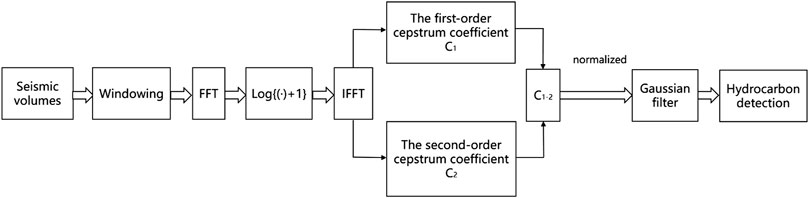
FIGURE 1. Seismic-print analysis flow.

Hydrocarbon detection technology based on the seismic-print analysis directly extracts the rock’s pore–fluid information from the seismic data, which do not explicitly involve the formation mechanism of the seismic response, and have no approximate problem with the numerical model. These features are the main differences between seismic-print analysis-based hydrocarbon detection technology and the other hydrocarbon detection technologies based on forward modeling and the inversion of the wave equation.

Figure 2 shows the seismic-print characteristics of two seismic sections intersecting different wells: gas well (Figure 2A) and dry well (Figure 2B) from marine carbonate reservoirs in Sichuan, China. The target horizon is shown by a green line. The first- and second-order cepstrum coefficients’ volumes of the seismic section intersecting gas well show the mirror symmetry relations in the reservoir area as shown by a rectangular box in Figures 2C,E while the first- and second-order cepstrum coefficients’ volumes of the seismic section intersecting the dry well do not represent the similar characteristics as shown by Figures 2D,F. And the result of the new parameter C₁₋₂ is shown by Figures 2G,H.

FIGURE 2

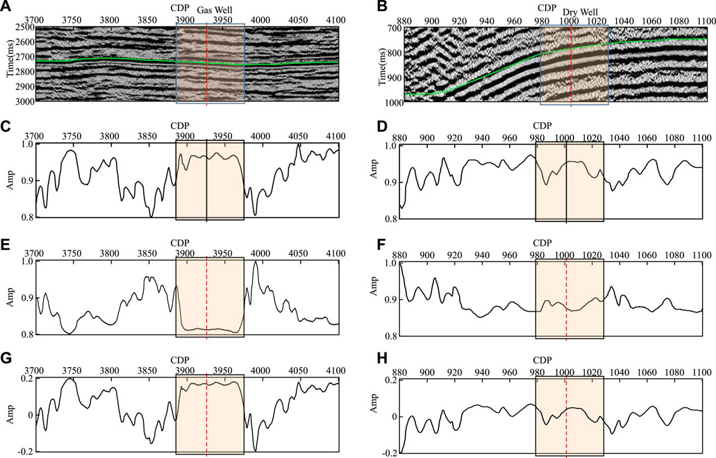
FIGURE 2. The Seismic-print characteristics of two seismic sections intersecting different wells. (A) The seismic section intersecting the gas well. (B) The seismic section intersecting the dry well. (C) The first-order cepstrum coefficient’s volume of the seismic section in (A). (D) The first-order cepstrum coefficient’s volume of the seismic section in (B). (E) The second-order cepstrum coefficient’s volume of the seismic section in (A). (F) The second-order cepstrum coefficient’s volume of the seismic section in (B). (G) The result of the new parameter C₁₋₂ in (A). (H) The result of the new parameter C₁₋₂ in (B).

3 Depth-Domain Seismic Dispersion Analysis

Since Futterman (1962) first discussed in detail that the absorption and attenuation of seismic waves by rocks (frequency dispersion phenomenon) is the fundamental characteristic of the formation, people have paid more and more attention to the attenuation of seismic waves. Winkler and Nur (1982) pointed out that the leading causes of seismic wave attenuation in rocks are friction, liquid flow, viscous relaxation, and diffusion. Different lithologies have different absorption degrees of seismic waves. The stronger the absorption of the stratum, the faster the attenuation of the high-frequency component of the seismic wave (Pujol and Smithson, 1991; Helle et al., 2003). According to the close relationship between formation absorption properties and lithofacies, porosity, and oil-gas composition, lithology can be predicted, and the existence of oil and gas can be directly predicted under favorable conditions (He et al., 2008). Dilay and Eastwood (1995) discussed the frequency spectrum inside, above, and below the reservoir and analyzed the influence of the hydrocarbon property on the power spectrum. The research and application practice shows that the frequency attenuation gradient is an attribute that is more sensitive to hydrocarbon reactions. According to the theory of viscoelasticity, the amplitude of seismic waves attenuates exponentially as the propagation distance of the seismic waves increases due to the absorption effect generated by uniform incompletely elastic media, that is,

$A=A_0{\mathrm{e}}^{-\alpha x},(10)$

where A is the amplitude of the seismic wave after propagating for a certain distance; A₀ is the initial amplitude of seismic wave; α is the absorption coefficient; and x is the propagation distance of seismic wave.

The absorption coefficient of different lithologies shows a colossal difference. For example, the absorption coefficient of sandstone layers is larger than that of other rock layers (such as limestone layers). Therefore, the spread of seismic waves in the long-distance, its amplitude decay is severe, especially when with the underlying cracks in filling the hydrocarbon, the amplitude attenuation is more intense, which is the theoretical basis for applying the frequency attenuation property to predict the hydrocarbon properties of the formation (Berryman and Wang, 2000).

At present, the measurement of dispersion is carried out in the time domain, but the time-domain dispersion has the problem of inaccurate construction (Wu et al., 2007), and the time profile and depth profile will not be completely consistent. Because of the speed difference, the depth with higher speed is greater than the depth with lower speed in the same second and the time profile and depth profile will not be completely consistent. Because of the speed difference, the depth with higher speed is greater than the depth with lower speed in the same second as shown in Figure 3, within the same depth interval in the depth domain (e.g., 120 m, due to different rock velocities (e.g., 5 and 4 km/s respectively), The thickness of the form shown on the seismic profile in the time domain can vary widely (in the case of 48 and 60 ms (two-way travel time), a difference of 12 ms), and the dispersion measured in the time domain can be used to estimate the spatial distribution of the reservoir, resulting in incorrect results.

FIGURE 3

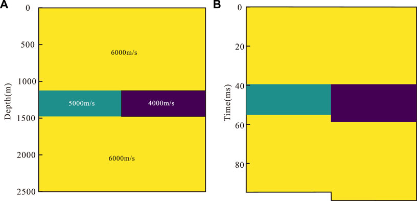
FIGURE 3. Model comparison diagram. (A) Depth-domain model. (B) Time-domain model.

Depth-domain seismic attributes are similar to time-domain seismic attributes in that they derive special measurements of geometry, kinematics, dynamics, and statistical characteristics from seismic data. The dynamic attributes reflect the amplitude variation of seismic data and the variance, gradient, and energy curvature extended by the amplitude (energy) (Singh, 2012; Zhang et al., 2017). The meaning of the depth domain is consistent with that of the time domain. Also, due to the more accurate positioning of imaging points in the depth domain, the more accurate spatial position of the measured attributes can better serve the reservoir prediction (Zhang et al., 2017; Cavalca et al., 2015).

3.1 Time-Depth Conversion of Seismic Data

The time-depth conversion converts a two-way time-domain seismic record to the depth domain, in effect transforming a time-domain seismic wavelet into a depth-domain seismic wavelet. A discrete expression for a two-way time–sine decay wavelet in the time domain is given as

$\begin{array}{cc}\hfill & x_w\left(i\mathrm{\Delta }t\right)=A_0{e}^{-ai\mathrm{\Delta }t}\sin 2\pi \left(f_m-f_{n}i/N\right)i\mathrm{\Delta }t\left(i=0,\dots ,N\right)\hfill \end{array},(11)$

where f_m and f_n denote the starting principal frequency and frequency decay values of the wavelet, respectively; α is the time decay exponents; and N is the number of wavelet points. Similarly, we also give a discrete expression for the depth-domain sinusoidal decay wavelet:

$\begin{array}{cc}\hfill & y_w\left(iM\right)=A_0{e}^{-\beta i\mathrm{\Delta }h}\sin 2\pi \left(k_m-k_{n}i/N\right)iAh\left(i=0,\dots ,N\right)\hfill \end{array},(12)$

where k_m and k_n denote the initial main wave number and the wave number attenuation value of the wavelet, respectively, β is the spatial attenuation index, which is desirable for the sake of consistency βΔh = αΔt.

Since the time domain is two-way time and the depth domain is one-way depth, the frequency of the time domain to the wave number of the depth-domain conversion relation should not be the usual relation:

$f=kv.(13)$

Also, it should be written as

$f=\frac{1}{2}kv.(14)$

Here v is the time-depth velocity of logging interpretation, f is the frequency, and k is the wave number. So, Eq. 11 can also be written as

$\begin{array}{cc}\hfill y_w\left(i\mathrm{\Delta }h\right)& =A_0{e}^{-\beta i\mathrm{\Delta }h}\sin 2\pi \left(f_m-f_{n}i/N\right)i2\mathrm{\Delta }h/v\hfill \\ \hfill & =A_0{e}^{-ai\mathrm{\Delta }t}\sin 2\pi \left(f_m-f_{n}i/N\right)i\mathrm{\Delta }t\hfill \end{array}.(15)$

From this, we get a conclusion that the sampling interval relation satisfies

$\mathrm{\Delta }t=2\mathrm{\Delta }h/v.(16)$

Then, after the wavelet frequency in the time domain is given, the wavelet in the time domain and the depth domain are numerically equal, that is,

$x_w\left(i\mathrm{\Delta }t\right)=y_w\left(i\mathrm{\Delta }h\right).(17)$

3.2 Calculation Method of Seismic Dispersion Attenuation in the Depth Domain

Mitchell et al. (1996) proposed an analysis method for calculating the energy attenuation of a seismic signal. The core of this technology is to obtain the high-frequency exponential attenuation coefficient of the signal spectrum. Due to the attenuation of waves during propagation, seismic waves are expressed as

$A=A_0{\mathrm{e}}^{-ax}{\mathrm{e}}^{\mathrm{i}\left(k_{x}x\pm ut\right)},(18)$

where k_r = k − iα, k is the plural; α is the attenuation coefficient of the signal, which is also what we want to calculate. The calculation process of the energy absorption analysis (EAA) technology is to continuously analyze the spectrum of seismic channels with a series of small windows and calculate the attenuation coefficient. The guiding ideology of EAA technology is to eliminate regular and uniform energy attenuation in the spectrum analysis to retain the abnormal part of attenuation.

The depth-domain-specific algorithm of EAA is as follows: first of all, for each seismic record do a depth frequency analysis (Figure 4A), on the deep frequency section detect the maximum energy frequency as the initial attenuation frequency (Figure 4B), then calculate the frequency corresponding to 20 and 95% of the seismic wave energy and the corresponding frequency in the frequency range, according to the frequency of the corresponding energy, fitting of the frequency and energy attenuation gradient. The amplitude attenuation gradient factor is obtained (Figure 4C). The process of EAA dispersion measurement method based on the aforementioned steps is shown in Figure 5. The main key points are the conversion of depth-domain data and the extraction of dispersion parameters.

FIGURE 4

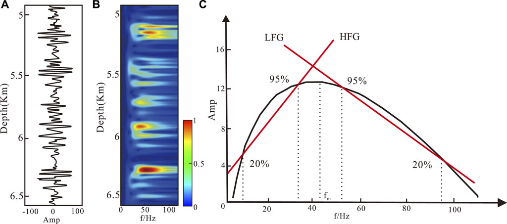
FIGURE 4. Diagram of the EAA calculation method in the depth domain. (A) Deep seismic gathers; (B) depth time–frequency analysis diagram; (C) EAA extraction instructions.

FIGURE 5

FIGURE 5. Flow of the depth-domain seismic wave frequency dispersion analysis.

4 Seismic Deep Learning

The advent of the era of artificial intelligence provides new ideas and methods for many hydrocarbon exploration problems. Deep learning forms more abstracted high-level attribute categories or feature representations through a layer-by-layer combination of low-level features, so it can deeply dig into the essential information of data and show its unique advantages and characteristics in recognition and classification (Goodfellow et al., 2016). At present, the main applications of deep learning in seismic exploration are fault recognition (Gan et al., 2016), first arrival picking (Liao et al., 2019), noise suppression (Liu et al., 2018), and velocity model construction (Yang and Ma, 2019), which have good results. Gao et al. (2020) using the transfer learning method for seismic reservoir gas prediction, Song et al. (2022) proposed a kNN-based gas-bearing prediction method by k nearest neighbor (kNN) method, both having good results. Through the block processing of seismic images and combining the respective characteristics of supervised and unsupervised learning, it is successfully applied in the hydrocarbon identification of 3D seismic data. These successful examples have laid the advantages of deep learning in establishing the non-linear mapping relationship between two datasets. At present, there are few applications in gas prediction, so the introduction of deep learning to hydrocarbon detection has a long-term development significance. Pre-stack seismic data have always been the key data basis for hydrocarbon detection. The amplitude change information contained in one time point of pre-stack data includes reservoir gas and water information, which is also the theoretical basis of AVO inversion. If the relationship between pre-stack data and hydrocarbon is to be established directly, the quality of pre-stack data is particularly important. To solve this problem, we also developed a pre-stack trace set optimization method based on bi-dimensional empirical mode decomposition (BEMD) to improve the effective information of the trace set and enhance the matching degree with a gas-bearing property (Jiang et al., 2020a), and the method of removing the strong reflection prominent effective signal (Jiang et al., 2021). The network selects the fully-connected network to deeply mine information and establish the non-linear mapping relationship between pre-stack data and hydrocarbon.

4.1 Overview of Deep Neural Network Algorithms

Establish the relationship between the labeled dataset and the training dataset using a deep neural network algorithm (DNN) to form a prediction network. Neural network technology originated in the fifties and sixties of the last century, called perceptron, with input, output, and a hidden layer. The input feature vector is transformed to the output layer through the hidden layer, and the classification results are obtained at the output layer. DNN can be understood as a neural network with many hidden layers. According to the position of the different layers, the inner neural network layer of DNN can be divided into three categories: input layer, hidden layer, and output layer. Generally speaking, the first layer is the input layer, the last layer is the output layer, and the middle layer is the hidden layer. One layer and another layer are fully connected, in other words, any neuron in layer i must be connected with any neuron in layer i+1. Although DNN looks pretty complex, it is still the same as perceptron from a small local model, that is, a linear relationship:

$z=\sum w_i{x}_i+b,(19)$

where z is the output layer, w_i is the weight value, x_i is the input layer, b is the bias, and then the final activation function σ(z) is added to form the basic structure of DNN. DNN is a neural network algorithm with multiple hidden layers. In the forward propagation phase, the hidden layer takes the output of the former layer as the input for the latter layer:

$b_k^L=\sum _{i=0}^n{w}_{\bar{i}}^L\cdot a_i^{L-1}+d_k^L,(20)$

$a_k^L=f\left(b_k^L\right),(21)$

where $b_k^L$ represents the output before the activation of the k neurons in the L layer of DNN, $a_k^L$ represents the output after the activation of the k neurons in the L layer of DNN, $w_{ik}^L$ represents the linear transfer coefficient from $a_i^{L-1}$ to $b_k^L$, $d_k^L$ represents the bias constant of the forward propagation function of $b_k^L$, and f is the activation function. Select Relu function as activation function. Firstly, the Relu function is one of the common activation functions expressed as follows:

$f\left(x\right)=\max \left(0,x\right).(22)$

The Relu function is a piecewise linear function, which changes all negative values to 0, while the positive values remain unchanged. This operation is called a unilateral suppression. If the input is negative, the output will be 0. The neuron will not be activated, which means that only part of the neurons will be started simultaneously, making the network very sparse and efficient for computing. Taking pre-stack seismic data as inputs and hydrocarbon as labels, a direct non-linear mapping relationship is established through the multi-hidden full connection network (DNN) to realize hydrocarbon detection. Similarly, when we input AVO features as labels, we can take a certain time window vertically and select AVO features within the time window as input features, such as 5 ms, which will help to improve the stability and continuity of the results. The network structure is shown in Figure 6. The number of network layers and neurons can be set according to the complexity of the data to improve the adaptability and accuracy of the algorithm.

FIGURE 6

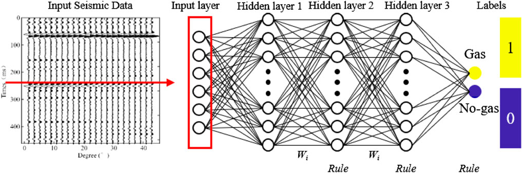
FIGURE 6. DNN network structure.

4.2 The Construction Principle of the Gas Prediction Method Based on Deep Neural Network

The classical AVO inversion analysis theory builds a non-linear relationship between amplitude variation with offset and gas-bearing properties. However, due to the universality of the mapping relationship established by the classical method and the strong approximation of the non-linear mapping relationship, the prediction accuracy is often low, and the adaptability is worse under deep conditions. The continuous development of deep neural networks in recent years has shown a unique advantage in non-linear mapping problems. Therefore, according to the relationship between AVO characteristics and the gas-bearing property, the deep neural network is selected as a bridge to build its non-linear relationship. Combined with the traditional AVO analysis technology, the calculation accuracy and efficiency are improved. Based on AVO characteristics, the input layer of the deep neural network is defined as the amplitude variation of the processed gather with offset, and the gas-bearing and non-gas-bearing results of the output layer are the output. A multi-layered deep neural network structure is defined. The whole algorithm flow is shown in Figure 7. The deep neural network algorithm greatly simplifies the screening process of the traditional AVO analysis method. It directly establishes the non-linear mapping relationship between pre-stack gather and hydrocarbon. The results obtained through the established network reduce the interference of human factors and improve the accuracy and reliability of the results.

FIGURE 7

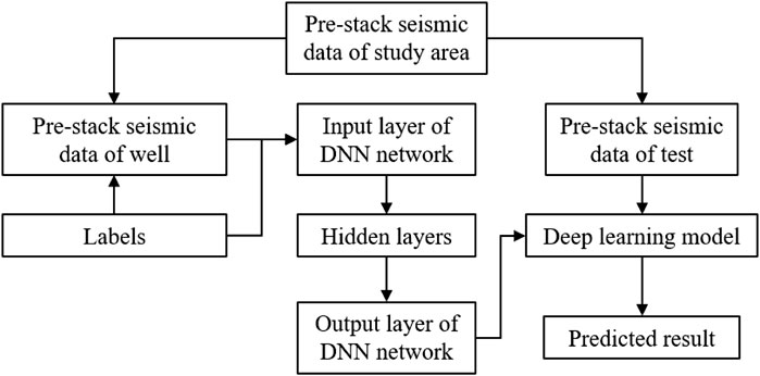
FIGURE 7. Flow chart of DNN hydrocarbon detection method.

5 A Case Study

5.1 Area Introduction

The study area is located in the Xiaoquan–Xinchang tectonic belt of the western Sichuan exploration area, with 150 km² as shown in Figure 8. The Xiaoquan–Xinchang tectonic zone is mainly zonal distribution located in the Longmenshan foreland basin. Among them, the collision and contact area of the Qinghai–Tibet Plateau and the Yangtze Block, two important tectonic parts of China, is the Longmenshan thrust belt–Longmenshan foreland basin mountain basin system. The specific shape of the Longmenshan foreland basin is a general zonal depression located at the core of China’s abundant natural gas resources. It gradually appeared in the Late Triassic period. The thickness of the continental debris deposited in the basin differed, and some areas could be more than 5,000 m. The main target interval was the deep carbonate rock of the Leikoupo Formation. Three wells have been drilled in the study area, and the seismic profile of the wells is shown in Figure 9 where T2l41 is the top of the upper reservoir of the fourth member of the Leikou profile group, and T2l43 is the bottom of the lower reservoir of the fourth member of the Leikoupo group. T2l4 is the bottom of the fourth member of the Leikoupo Formation, and T2l3 is the bottom of the third member of the Leikoupo Formation. The main target interval of this study is T2l41 – T2l43. From the seismic profile, it can be seen that the reservoir is thin, and the signal is relatively weak, and the seismic signal difference of the three wells is small. Well A, well B, and well C’s drilling profiles are shown in Figure 10. The drilling section mainly shows the upper and lower reservoir information of the upper sub-member of the fourth Leikoupo formation. From the logging interpretation results, the reservoir location contains many thin reservoirs, and the reservoir conditions are good, but the drilling results showed that not all of the high quality reservoirs contain gas. Well B had a good gas-bearing property in the upper sub-member of the fourth Leikoupo formation, well A was a water well, well C was a gas–water mixed well; well C had a good gas-bearing property in the upper and lower reservoirs of the fourth Leikoupo formation, well A was still a water well, and well B had a relatively weak gas-bearing property. Both seismic data and drilling profiles show the difficulty of hydrocarbon detection, and also indicate the demand for gas prediction.

FIGURE 8

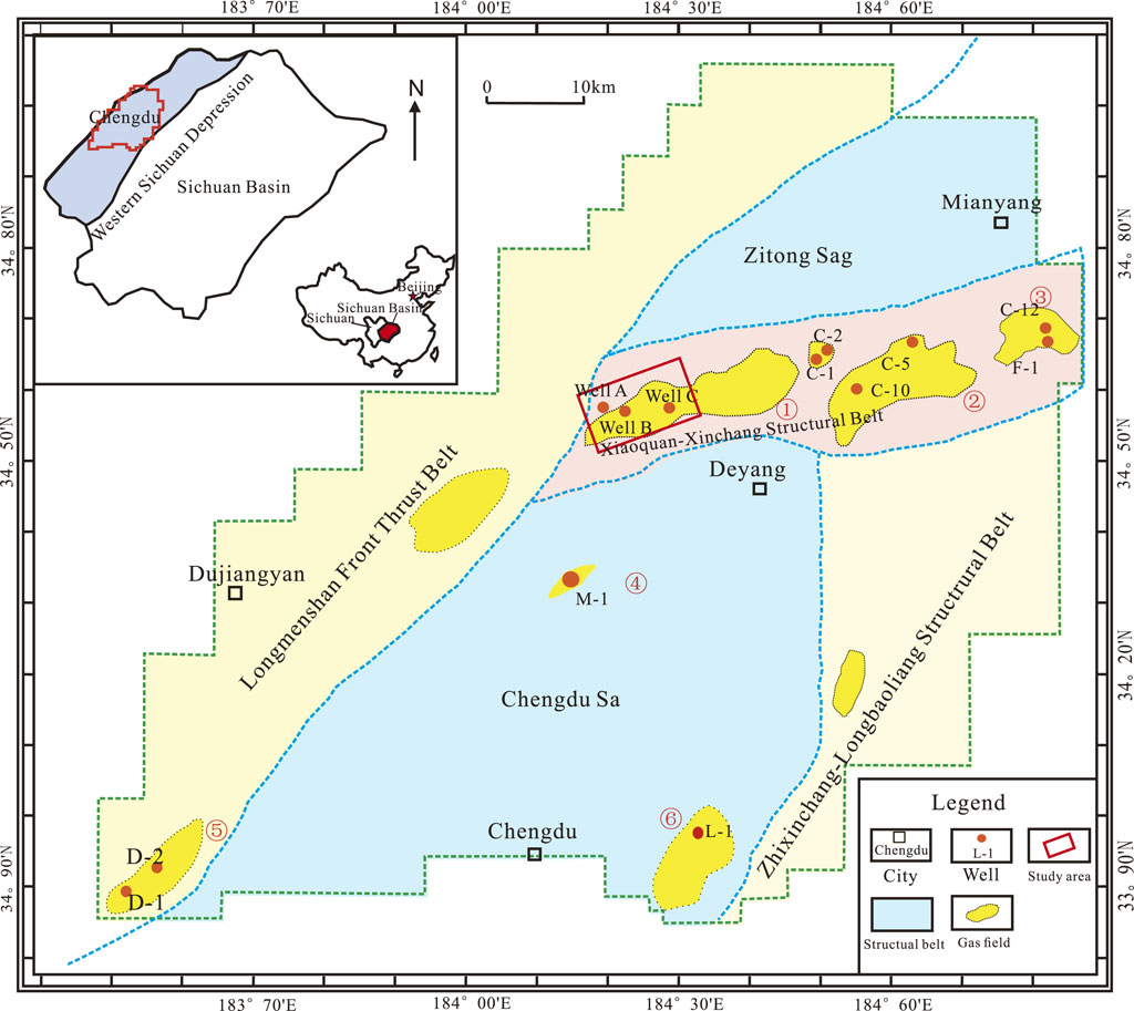
FIGURE 8. Structural diagram of study area.

FIGURE 9

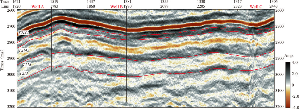
FIGURE 9. Seismic profile of the wells in the study area.

FIGURE 10

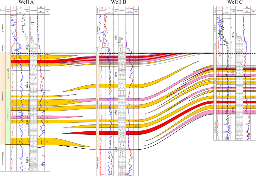
FIGURE 10. Profile of the drilled wells in the study area.

5.2 Results

5.2.1 Seismic-Print Analysis

The seismic-print analysis method is used to calculate the profile in the study area, and the hydrocarbon detection results are obtained. In Figure 11, the strong amplitude anomaly area indicates that in the hydrocarbon area, the stronger the amplitude, the stronger the hydrocarbon. It can be seen from the results in T2l41–T2l43 that Well A is a water well, and the amplitude anomaly is relatively weak, which is consistent with the results. The hydrocarbon of wells B and C shows a strong amplitude anomaly. The strong amplitude anomaly position is in good agreement with the hydrocarbon position, and the overall hydrocarbon detection distribution is in good agreement with the geological distribution characteristics, which verifies the method’s effectiveness.

FIGURE 11

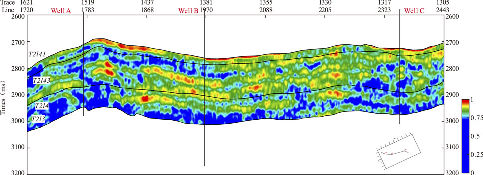
FIGURE 11. Seismic-print analysis result.

5.2.2 Depth-Domain Seismic Dispersion Analysis

Firstly, the time-depth conversion of the seismic data is carried out to obtain the results of Figure 12. It can be seen that after conversion, the actual structural distribution of the three wells is more conducive to gas distribution and migration and a more intuitive display of reservoir distribution. The EAA algorithm is used to calculate the dispersion based on the depth-domain data, and the results are shown in Figure 13. The same strong amplitude represents the gas-bearing strength. The results further demonstrate the non-hydrocarbon nature of well A and the hydrocarbon nature of wells B and C, which have a higher accuracy and can measure the hydrocarbon to some extent in the horizon from T2l41 to T2l43.

FIGURE 12

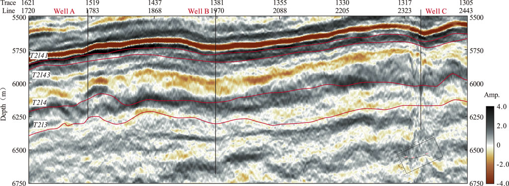
FIGURE 12. Results of the profile after time-depth conversion.

FIGURE 13

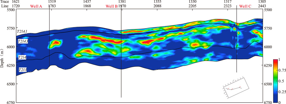
FIGURE 13. Prediction results of depth threshold dispersion hydrocarbon.

5.2.3 Seismic Deep Learning

The pre-stack seismic gathers of well B and well C are used to establish a training dataset corresponding to the gas-bearing property after time-depth conversion (1 is gas-bearing, 0 is non-gas-bearing). The dataset size is 24,000 training samples (using the whole profile data set, the profile time range is 2,400–3,600 ms, and the number of samples corresponding to a single well is 1200. The five pre-stack gathers before and after the two wells are used as training data to form a training set of 10*1200 = 24,000 samples). The whole profile is used as a prediction sample containing 340,800 prediction samples. A deep neural network with five hidden layers is established. The activation function selects a sigmoid function, the number of neurons is 200, the loss rate of neurons is 0.6, the single training batch size of training samples is 45, and the number of iterations is 1,000. Labels 0 and 1 are the label calibrations of gas-bearing and non-gas-bearing reservoirs. The sigmoid function is used as the activation function to distribute the predicted results [0, 1]. Thus, the predicted results represent a probability closer to gas-bearing and non-gas-bearing reservoirs. When drawing, all values below 0.5 are set as non-gas-bearing, and values above 0.5 are expressed in an increasingly red color, and the profile results of hydrocarbon detection results are obtained, as shown in Figure 14. It can be seen from the results that the overall hydrocarbon prediction results are highly consistent with the drilling results and geological laws. The test results show that well A is a water layer in T2l41–T2l43. Well B has strong gas-bearing characteristics in the upper section of the fourth member of the Leikoupo section. The overall results are consistent with the drilling results, especially well A without network training, and the results are also consistent with the actual, indicating the effectiveness and stability of the neural network algorithm.

FIGURE 14

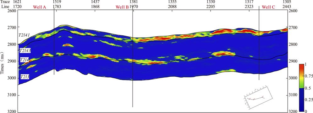
FIGURE 14. DNN hydrocarbon detection results.

5.2.4 Three-Dimensional Data Analysis

Based on the two-dimensional profile calculation results, three methods are used to predict the slicing results of the upper reservoir of the Leikoupo fourth section, the lower reservoir of the Leikoupo fourth section, and the Leikoupo third section in the three main target horizons of the whole area. Figures 15A,C, and E are the hydrocarbon prediction results of the upper sub-member fourth of the Leikoupo Formation, and b,d, and f are the lower members, Figures 15A,C, and E represent the seismic-print analysis method, depth-domain dispersion, and the DNN network method, and Figures 15B,D, and F correspond to the meanings of a, c, and e. The upper and lower reservoir prediction results show the effectiveness and consistency of the three methods. The upper reservoir results show the characteristics of well A without gas, well B with gas, and well C with the gas–water mixture, while the lower reservoir results show the characteristics of well A without gas, well B with gas, and well C with gas. The predicted results are consistent with the actual drilling results, indicating the effectiveness of the proposed method.

FIGURE 15

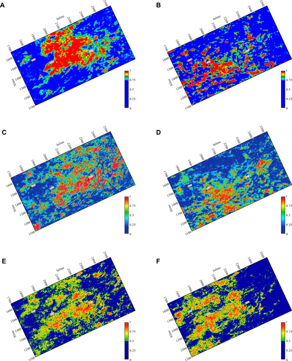
FIGURE 15. Three dimensional result of hydrocarbon detection. (A) Seismic-print analysis of hydrocarbon detection results for upper member 4 of the Leikoupo Formation (T2l41). (B) Seismic-print analysis of hydrocarbon detection results for the lower reservoir section of the fourth member of the Leikoupo Formation (T2l43). (C) Prediction results of the dispersion hydrocarbon in depth domain of upper reservoir section 4 of the Leikoupo Formation (T2l41). (D) Prediction results of dispersion hydrocarbon in depth domain of lower member 4 of the Leikoupo Formation (T2l43). (E) Prediction results of hydrocarbon in DNN of upper member 4 of the Leikoupo Formation (T2l41). (F) Prediction results of the hydrocarbon capacity of DNN of lower reservoir Section 4 of the Leikoupo Formation (T2l43).

5.3 Discussion

The burial depth of the carbonate strata of the Leikoupo Formation in the study area is more than 5,500 m, and the thickness of a single reservoir is several meters to 10 m. The physical properties of the gas-bearing reservoirs and water-bearing reservoirs are small, making the detection of gas-bearing reservoirs based on seismic data prone to errors. Before drilling, all the wells have been used for reservoir prediction and gas-bearing detection using the most advanced methods and technologies, including the failed well which is low in production. Even after drilling, the test results are still not completely consistent with the actual drilling results of some wells by adding the well data constraints. This shows that the existing gas detection methods cannot meet the exploration needs in deep, complex reservoir conditions. From the experimental results introduced in the previous section, the detection results of our newly developed reservoir hydrocarbon detection method are highly consistent with the actual drilling results. The seismic deep learning (SDL) method has higher accuracy, but the calculation cost is high. In comparison, the seismic-print analysis (SPA) method has higher efficiency. The depth-domain seismic dispersion analysis (DDSDA) method has more practical significance and can accurately predict the gas-bearing depth and location. This shows that the new method can better adapt to strong heterogeneity and weak seismic response of the ultra-deep ancient carbonate reservoir medium. The main advantage of the new methods is that they are data-driven and do not need to model rock physics and seismic response mechanisms, so they can naturally adapt to any complex medium. In contrast to the DHI methods such as AVO analysis, the calculation expression of evaluation parameters has made many assumptions in derivation. If the actual situation does not coincide with these assumptions, it may be wrong. At the same time, we should also see that the evaluation standard of data-driven reservoir hydrocarbon detection depends on the calibration of well data. When the available well data are few, or no well data are available at all, it is possible to make mistakes according to experience. But, we believe that with the accumulation of practical application data, the reliability of data-driven reservoir gas detection methods will be higher and higher. Data-driven reservoir gas-bearing detection results are essentially probabilistic and, in most cases, qualitative. The success of oil and gas exploration wells depends on quantity. Only when the product reaches the level of economic benefits can it be called a success. Therefore, the evaluation of reservoir hydrocarbon should develop from qualitative detection to quantitative prediction in the future, and the technology of reservoir hydrocarbon prediction should be developed. The existing drilling data reveal that the ultra-deep ancient carbonate reservoir has strong heterogeneity. At the same time, due to deep burial and other reasons, the seismic response of the reservoir is weak and complex, so that the prediction of reservoir hydrocarbon based on rock physics and seismic response analysis modeling is almost impossible. Deep network adaptive non-linear modeling based on deep learning can play a role, which may be the most potential breakthrough research.

In general, this article studies and discusses the current hydrocarbon prediction methods for deep and ultra-deep carbonate rocks. The seismic-print method is mainly for post-stack data, which can quickly and efficiently obtain weak gas-bearing information, but require a relatively high signal-to-noise ratio for post-stack data. The noise immunity is not particularly good. The depth-domain attenuation method can detect hydrocarbon from a depth perspective, making the prediction results more accurate, but the accuracy of time-depth conversion needs to be improved; the neural network hydrocarbon prediction is based on pre-stack data, which improve the efficiency and accuracy of calculation, but the establishment of a sample database is still a problem that needs to be further studied.

6 Conclusion

This article describes three methods for gas reservoir identification of ultra-deep carbonate rocks in the Sichuan Basin: seismic-print analysis method, depth-domain dispersion analysis method, and seismic deep learning method. The seismic-print analysis method uses cepstrum analysis to highlight the reservoir’s weak response signal and reveal the cepstrum characteristics of the gas-bearing reservoir. The first-order and second-order cepstrum coefficient anomalies are a convex mirror symmetry. The depth-domain dispersion analysis method converts the dispersion analysis usually carried out in the time domain to the real space domain, creating conditions for estimating the reservoir hydrocarbon based on dispersion. The seismic deep learning method uses the adaptive non-linear modeling ability of a complex system of the deep network to construct the deep network model that directly predicts reservoir hydrocarbon from pre-stack seismic data. These three methods can be regarded as data-driven reservoir hydrocarbon detection methods, which do not explicitly involve establishing rock physical and seismic response analysis models. Therefore, compared with the existing DHI method, the applicability of these methods to the weak seismic response of ultra-deep strong heterogeneous reservoirs is stronger. The practical application results also demonstrate that these methods are more effective. Nevertheless, it is still not a silver bullet, and there is still a situation where the prediction results are not consistent with the actual situation, and it has not been widely applied.

Data Availability Statement

The original contributions presented in the study are included in the article/Supplementary Material; further inquiries can be directed to the corresponding author.

Author Contributions

Conception and design of study: JC, XJ, YX, RT, and MC. Acquisition of data: XJ, YX, and MC. Analysis and/or interpretation of data: XJ, YX, RT, and MC. Drafting the manuscript: XJ, YX, MC, and XT. Revising the manuscript critically for important intellectual content: XJ, YX, MC, and TX. Approval of the version of the manuscript to be published: JC, XJ, YX, RT, MC, and TX.

Funding

This work was supported by the National Natural Science Foundation of China (Grant Nos. 42030812, 41974160, and 41430323), project of the SINOPEC Science and Technology Department (Grant No. P20055-6), and Special Project of the Local Science and Technology Development guided by the Central Government in Sichuan (2021ZYD0030).

Conflict of Interest

The authors declare that the research was conducted in the absence of any commercial or financial relationships that could be construed as a potential conflict of interest.

The reviewer JX declared a shared affiliation with the authors, JC, XJ, RT, TX, and MC to the handling editor at the time of the review.

Publisher’s Note

All claims expressed in this article are solely those of the authors and do not necessarily represent those of their affiliated organizations, or those of the publisher, the editors, and the reviewers. Any product that may be evaluated in this article, or claim that may be made by its manufacturer, is not guaranteed or endorsed by the publisher.

References

Berryman, J. G., and Wang, H. F. (2000). Elastic Wave Propagation and Attenuation in a Double-Porosity Dual-Permeability Medium. Int. J. Rock Mech. Min. Sci. 37, 63–78. doi:10.1016/s1365-1609(99)00092-1

CrossRef Full Text | Google Scholar

Campbell, J. P. (1997). Speaker Recognition: A Tutorial. Proc. IEEE 85, 1437–1462. doi:10.1109/5.628714

CrossRef Full Text | Google Scholar

Cao, J. (2017). Deep Learning and its Application in Deep Gas Reservoir Prediction. Comput. Tech. Geophys. Geochem. Explor. 39, 775–782.

Google Scholar

Cao, J., He, X., and Wu, S. (2017). Reservoir Detection Method Based on Deep Learning of Seismic Data. chinese invention patent: Zl 2017 1 0115720.6.

Google Scholar

Cao, J., Liu, S., Tian, R., Wang, X., and He, X. (2011a). Seismic Prediction of Carbonate Reservoirs in the Deep of Longmenshan Foreland Basin. Acta Petrol. Sin. 27, 2423–2434.

Google Scholar

Cao, J., Tian, R., and He, X. (2011b). Seismic-print Analysis and Hydrocarbon Identification. AGU Fall Meet. Abstr. 2011, S33B–S01.

Google Scholar

Cao, J., and Tian, R. (2011). Reservoir Detection Method Based on Seismic Pattern Analysis. chinese invention patent:zl 20111 0165615.6.

Google Scholar

Cao, J., and Wu, S. (2017). “Deep Learning: Chance and Challenge for Deep Gas Reservoir Identification,” in International Geophysical Conference, Qingdao, China, 17-20 April 2017 (Houston, Texas, USA: Society of Exploration Geophysicists and Chinese Petroleum Society), 711–712.

Google Scholar

Cao, J., Xue, Y., Tian, R., and Shu, Y. (2019). Advances in Hydrocarbon Detection in Deep Carbonate Reservoirs. Geophys. Prospecrting Petroleum (in Chinese) 58, 9–16.

Google Scholar

Cao, X. Y. J., and Tian, R. (2019). Advancesinhyg Drocarbon detectionindeepcarbonatereservoirs. Geophysical Prospecting for Petroleum 58, 9G–16G.

Google Scholar

Castagna, J. P., and Backus, M. M. (1993). Offset-dependent Reflectivity—Theory and Practice of AVO Analysis. Houston, Texas, USA: Society of Exploration Geophysicists.

Google Scholar

Castagna, J. P., Sun, S., and Siegfried, R. W. (2003). Instantaneous Spectral Analysis: Detection of Low-Frequency Shadows Associated with Hydrocarbons. The leading edge 22, 120–127. doi:10.1190/1.1559038

CrossRef Full Text | Google Scholar

Cavalca, M., Fletcher, R., and Du, X. (2015). “Q-compensation through Depth Domain Inversion,” in 77th EAGE Conference and Exhibition 2015 (Houten, Netherlands: European Association of Geoscientists & Engineers), 1–5. doi:10.3997/2214-4609.201413250

CrossRef Full Text | Google Scholar

Chopra, S., and Castagna, J. (2014). Avo (Investigations in Geophysics Series No. 16). Houston, Texas, USA: Society of exploration geophysicists.

Google Scholar

Cui, C.-j., Gong, Y.-j., and Shen, D.-y. (2010). Application of Wave Impedance Inversion to Reservoir Prediction Research. Progress in Geophysics 25, 9–15.

Google Scholar

Das, R. K., and Prasanna, S. R. M. (2018). Speaker Verification from Short Utterance Perspective: a Review. IETE Technical Review 35, 599–617. doi:10.1080/02564602.2017.1357507

CrossRef Full Text | Google Scholar

Dilay, A., and Eastwood, J. (1995). Spectral Analysis Applied to Seismic Monitoring of Thermal Recovery. The Leading Edge 14, 1117–1122. doi:10.1190/1.1437081

CrossRef Full Text | Google Scholar

Fawad, M., Hansen, J. A., and Mondol, N. H. (2020). Seismic-fluid Detection-A Review. Earth-Science Reviews 210, 103347. doi:10.1016/j.earscirev.2020.103347

CrossRef Full Text | Google Scholar

Futterman, W. I. (1962). Dispersive Body Waves. J. Geophys. Res. 67, 5279–5291. doi:10.1029/jz067i013p05279

CrossRef Full Text | Google Scholar

Gan, M., Wang, C., and Zhu, C. a. (2016). Construction of Hierarchical Diagnosis Network Based on Deep Learning and its Application in the Fault Pattern Recognition of Rolling Element Bearings. Mechanical Systems and Signal Processing 72-73, 92–104. doi:10.1016/j.ymssp.2015.11.014

CrossRef Full Text | Google Scholar

Gao, J., Song, Z., Gui, J., and Yuan, S. (2020). Gas-bearing Prediction Using Transfer Learning and Cnns: An Application to a Deep Tight Dolomite Reservoir. IEEE Geoscience and Remote Sensing Letters 19.

Google Scholar

Goodfellow, I., Bengio, Y., and Courville, A. (2016). Deep Learning. Cambridge, MA, USA: MIT press.

Google Scholar

Hammond, A. L. (1974). Bright Spot: Better Seismological Indicators of Gas and Oil. Science 185, 515–517. doi:10.1126/science.185.4150.515

PubMed Abstract | CrossRef Full Text | Google Scholar

He, X., Cao, J., and X, J. (2018). A Reservoir Gas-Bearing Evaluation Method Based on Seismic Wave Dispersion Analysis in Depth Domain. chinese invention patent, zl 201811388697.9.

Google Scholar

He, Z., Xiong, X., and Bian, L. (2008). Numerical Simulation of Seismic Low-Frequency Shadows and its Application. Appl. Geophys. 5, 301–306. doi:10.1007/s11770-008-0040-4

CrossRef Full Text | Google Scholar

Helle, H. B., Pham, N. H., and Carcione, J. M. (2003). Velocity and Attenuation in Partially Saturated Rocks: Poroelastic Numerical Experiments. Geophysical Prospecting 51, 551–566. doi:10.1046/j.1365-2478.2003.00393.x

CrossRef Full Text | Google Scholar

Jiang, X., Cao, J., Hu, J., Xiong, X., and Liu, J. (2020a). Pre-stack Gather Optimization Technology Based on an Improved Bidimensional Empirical Mode Decomposition Method. Journal of Applied Geophysics 177, 104026.

Google Scholar

Jiang, X., Cao, J., Yang, J., Liu, J., and Zhou, P. (2020b). Avo Analysis Combined with Teager-Kaiser Energy Methods for Hydrocarbon Detection. IEEE Geoscience and Remote Sensing Letters 19, 1–5.

Google Scholar

Jiang, X., Cao, J., Zu, S., Xu, H., and Wang, J. (2021). Detection of Hidden Reservoirs under Strong Shielding Based on Bi‐dimensional Empirical Mode Decomposition and the Teager-Kaiser Operator. Geophysical Prospecting 69, 1086–1101. doi:10.1111/1365-2478.13073

CrossRef Full Text | Google Scholar

Jin, S., Cambois, G., and Vuillermoz, C. (2000). Shear‐wave Velocity and Density Estimation from PS-Wave AVO Analysis: Application to an OBS Dataset from the North Sea. Geophysics 65, 1446–1454. doi:10.1190/1.1444833

CrossRef Full Text | Google Scholar

Kersta, L. G. (1962). Voiceprint Identification. The Journal of the Acoustical Society of America 34, 725. doi:10.1121/1.1937211

CrossRef Full Text | Google Scholar

Li, J., and Zhang, J. (2021). “A Study of Voice Print Recognition Technology,” in 2021 International Wireless Communications and Mobile Computing (IWCMC) (Harbin City, China: IEEE), 1802–1808. doi:10.1109/iwcmc51323.2021.9498681

CrossRef Full Text | Google Scholar

Li, X., Guo, J., Zhang, Q., and Tong, K. (2008). Determining Method for the Lower Limit of Physical-Property Parameters in Gas Reservoirs. Natural Gas Exploration and Development 31, 33–38.

Google Scholar

Liao, X., Cao, J., Hu, J., You, J., Jiang, X., and Liu, Z. (2019). First Arrival Time Identification Using Transfer Learning with Continuous Wavelet Transform Feature Images. IEEE Geoscience and Remote Sensing Letters 17, 2002–2006.

Google Scholar

Liu, D., Wang, W., Chen, W., Wang, X., Zhou, Y., and Shi, Z. (2018). “Random Noise Suppression in Seismic Data: What Can Deep Learning Do?,” in SEG Technical Program Expanded Abstracts 2018 (Houston, Texas, USA: Society of Exploration Geophysicists), 2016–2020.

Google Scholar

Mitchell, J. T., Derzhi, N., Lichman, E., and Lanning, E. N. (1996). “Energy Absorption Analysis: A Case Study,” in SEG Technical Program Expanded Abstracts 1996 (Houston, Texas, USA: Society of Exploration Geophysicists), 1785–1788. doi:10.1190/1.1826480

CrossRef Full Text | Google Scholar

Pujol, J., and Smithson, S. (1991). Seismic Wave Attenuation in Volcanic Rocks from Vsp Experiments. Geophysics 56, 1441–1455. doi:10.1190/1.1443164

CrossRef Full Text | Google Scholar

Robinson, J. C. (1979). A Technique for the Continuous Representation of Dispersion in Seismic Data. Geophysics 44, 1345–1351. doi:10.1190/1.1441011

CrossRef Full Text | Google Scholar

Russell, B. H., Hedlin, K., Hilterman, F. J., and Lines, L. R. (2003). Fluid‐property Discrimination with AVO: A Biot‐Gassmann Perspective. Geophysics 68, 29–39. doi:10.1190/1.1543192

CrossRef Full Text | Google Scholar

Singh, Y. (2012). Deterministic Inversion of Seismic Data in the Depth Domain. The Leading Edge 31, 538–545. doi:10.1190/tle31050538.1

CrossRef Full Text | Google Scholar

Smith, G. C., and Sutherland, R. A. (1996). The Fluid Factor as an Avo Indicator. Geophysics 61, 1425–1428. doi:10.1190/1.1444067

CrossRef Full Text | Google Scholar

Song, Z., Yuan, S., Li, Z., and Wang, S. (2022). kNN-Based Gas-Bearing Prediction Using Local Waveform Similarity Gas-Indication Attribute - an Application to a Tight Sandstone Reservoir. Interpretation 10, SA25–SA33. doi:10.1190/int-2021-0045.1

CrossRef Full Text | Google Scholar

Veeken, P., and Silva, M. D. (2004). Seismic Inversion Methods and Some of Their Constraints. First break 22, 1013. doi:10.3997/1365-2397.2004011

CrossRef Full Text | Google Scholar

Winkler, K. W., and Nur, A. (1982). Seismic Attenuation: Effects of Pore Fluids and Frictional‐sliding. Geophysics 47, 1–15. doi:10.1190/1.1441276

CrossRef Full Text | Google Scholar

Wu, R., Zhu, H., Lin, B., and Xue, S. (2007). “Wavelet Analysis and Convolution in Depth Domain,” in 2007 SEG Annual Meeting (Richardson, TX, USA: OnePetro).

CrossRef Full Text | Google Scholar

Xue, Y.-j., Cao, J.-x., and Tian, R.-f. (2013). A Comparative Study on Hydrocarbon Detection Using Three EMD-Based Time-Frequency Analysis Methods. Journal of Applied Geophysics 89, 108–115. doi:10.1016/j.jappgeo.2012.11.015

CrossRef Full Text | Google Scholar

Xue, Y.-j., Cao, J.-x., Tian, R.-f., Du, H.-k., and Yao, Y. (2016). Wavelet-based Cepstrum Decomposition of Seismic Data and its Application in Hydrocarbon Detection. Geophysical Prospecting 64, 1441–1453. doi:10.1111/1365-2478.12344

CrossRef Full Text | Google Scholar

Xue, Y.-j., Cao, J.-x., and Tian, R.-f. (2014). EMD and Teager-Kaiser Energy Applied to Hydrocarbon Detection in a Carbonate Reservoir. Geophysical Journal International 197, 277–291. doi:10.1093/gji/ggt530

CrossRef Full Text | Google Scholar

Yang, F., and Ma, J. (2019). Deep-learning Inversion: A Next-Generation Seismic Velocity Model Building Method. Geophysics 84, R583–R599. doi:10.1190/geo2018-0249.1

CrossRef Full Text | Google Scholar

Zhang, R., Zhang, K., and Alekhue, J. E. (2017). Depth-domain Seismic Reflectivity Inversion with Compressed Sensing Technique. Interpretation 5, T1–T9. doi:10.1190/int-2016-0005.1

CrossRef Full Text | Google Scholar

Zong, Z., Yin, X., and Wu, G. (2013). Elastic Impedance Parameterization and Inversion with Young's Modulus and Poisson's Ratio. Geophysics 78, N35–N42. doi:10.1190/geo2012-0529.1

CrossRef Full Text | Google Scholar