Two Improved Acquisition Systems for Deep Subsurface Exploration

Present land seismic surveys mainly focus on acquiring reflection data. The maximum offset is usually 1–1.5 times the depth of targets. Limited offset results in that the acquired diving waves only penetrate the shallow parts of the Earth model, far from targets. Thus, the reflection data are used to build the deep part of the velocity model with migration velocity analysis. However, two issues challenge the success of velocity model building. First, incomplete information. Limited offsets lead to a narrow aperture of observation, which results in an under-determined inversion system. One manifestation is the trade-off between the depth of interfaces/reflectors and the average velocity above them. Second, low signal-to-noise (S/N) ratios. Complex near-surface conditions and geologic structures lead to low S/N ratios for reflection data, which fails to build velocity with reflection data. The fundamental solution to these two issues is to acquire better data with an improved acquisition system. In this work, we propose two types of modified geometries to enhance the penetration depth of the diving waves, especially the first arrivals, which can be used to build a deeper velocity model effectively. Type-I geometry adds extra sparse sources on the extension line of the normal acquisition geometry, whereas Type-II geometry deploys extra sparse receivers on the extension line. Consequently, the new acquisition system includes ultra-large offsets, which acquire diving waves from the deep subsurface. These diving waves, including waveform and first-break time, are particularly useful for recovering deeper velocity, which has paramount significance for the exploration of deep and ultra-deep hydrocarbon reservoirs. Synthetic and field data examples preliminarily demonstrate the feasibility of this improved acquisition system.

Introduction

Active-source seismic surveys are the main geophysical method for the exploration of subsurface geological structures and reservoir characteristics. Current seismic surveys are often designed to acquire the reflection waves, which are the seismic energy bounced back at the interfaces between rock layers. Since oil/gas reservoirs are mainly found in sedimentary rocks dominated by the flat layer feature, the seismic surveys set the maximum offset to 1–1.5 times the depth of targets (Yilmaz, 2001). As a result, the surveys are adequate for recording reflection data.

The conventional seismic data processes aim at utilizing reflections, especially primary reflections. Other types of events, including direct arrivals and refractions, are treated as noise; therefore, they are suppressed during data processing (Yilmaz, 2001). The main steps of the data processing include velocity model building and migration. The data processing can be performed either in the time domain or the depth domain. The time-domain data process is still popular because of its high efficiency and robustness. However, it suffers from low accuracy. Its migration profiles only show the travel time from the surface to the interfaces. Thus, the migration profiles do not provide the depth of the interfaces. In addition, time-domain migration assumes that the rocks are homogenous above an interface in the aperture of one common-middle-point (CMP) gather. Consequently, time-domain migration could produce artificial geological structures, especially in the region where the velocity possesses strong variation. Thus, time-domain migration results are inappropriate for tasks requiring high accuracy imaging, for example, bore well-drilling design.

By contrast, the depth-domain migration provides the image of geological structures matching the real world (Zhang and Sun, 2008; Liu et al., 2011; Li et al., 2021). Its migration profiles, therefore, are ideal for subsequent processes and interpretation. However, depth migration needs an accurate depth velocity. The migration velocity does not need to contain fine details but must provide an accurate background velocity, which gives the correct travel time and wave paths of reflections. Therefore, building the accurate migration velocity is crucial for depth migration. Limited by the offset, reflections are the only information source for building velocity reaching the depth of targets. Reflection-waveform inversion (RWI) (Xu et al., 2012; Wu and Alkhalifah, 2015; Zhou et al., 2015; Yao and Wu, 2017; Yao et al., 2020) and reflection-traveltime tomography (Sherwood et al., 1986; Kosloff et al., 1996) can be used to achieve this goal. Currently, reflection-traveltime tomography is the mainstream tool for velocity building in the industry. The principle is to utilize the move out residual to update the velocity above the selected reflection interfaces.

Two factors hamper the success of velocity building based on reflections: first, the trade-off between the depth of reflectors and velocity above reflectors. This phenomenon is illustrated in Figure 1: if a reflector is moved up/down by reducing/increasing the velocity above the reflector, the travel time keeps the same as that for the true depth and velocity. One symptom in practical applications is that the inverted velocity has strong fluctuation along the strata, which leads to artificial undulated reflectors in the migration image. This undulation becomes more severe in deep parts of the model than its shallow parts due to fewer data constraints as depth increases, for example, Figure 7A of Yao et al. (2019). The fundamental reason for this phenomenon is that inadequate information is used in the inversion. In other words, the inversion system is under-determined. To mitigate this issue, it is necessary to incorporate more information into the system. For instance, structural smoothing is a common constraint used for this purpose (Lewis et al., 2014; Yao et al., 2019).

FIGURE 1

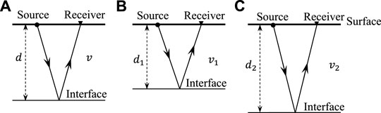
FIGURE 1. Schematic illustration for the trade-off between the depth of interface and velocity above it. (A) The true scenario: both depth $d$ and velocity $v$ are correct. (B) The trade-off scenario 1: $d_1<d$, $v_1<v$. (C) The trade-off scenario 2: $d_2>d$, $v_2>v$. The two trade-off scenarios give the same travel time as the true scenario.

The second factor is the low S/N ratio. This is common in land seismic surveys. Figure 2 shows one typical shot gather with a low S/N ratio. The reflection events are barely seen in the profile. The low S/N ratio is caused by the near-surface complexity and complex structures. Consequently, it is almost impossible to build a correct velocity model using reflections in such a scenario.

FIGURE 2

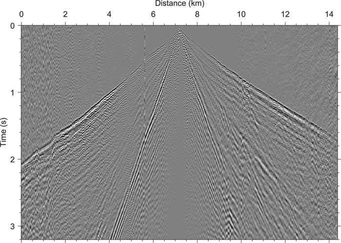
FIGURE 2. A typical shot profile acquired from the foothills around the Tarim Basin. Trace equalization was applied. Reflection events are barely seen while the first arrival is clear.

These two factors lead to a paradox: time migration gives even better migration images than depth migration in this type of scenario, but the migration theory tells that depth migration is more accurate than time migration. One reason why time migration works better here is that it can build an optimal velocity by scanning the semblance of stacking velocity, resulting in plausible migration images.

The analysis above indicates that building an accurate velocity model is the key to reliable depth migration. To achieve this goal, the fundamental solution is to acquire adequate and reliable data. The company BP set such a pioneering example for full-waveform inversion (FWI). BP created a marine vibrator, called WolfSpar, which can generate reliable signals as low as about 1.6 Hz at an offset of 30 km (Dellinger et al., 2016). By combining with ocean bottom nodes (OBN), the acquired dataset successfully delivered much more accurate velocity models with FWI than with reflection travel-time tomography, resulting in stunning migration images (Shen et al., 2018; Zhang et al., 2018).

In this article, we propose an improved acquisition system for building more reliable velocity models for deep subsurface exploration. The basic idea is to add extra spare sources or receivers along the extension line of the normal geometry. As a result, this acquisition system includes ultra-large offsets, which are the foundation to acquire diving waves from the deep subsurface. The diving waves are refraction waves that bend back to the surface due to the velocity gradient of the Earth (Sheriff, 2002). Their waveform and first-arrival time are particularly useful for recovering deeper velocity, which has paramount significance for the exploration of deep and ultra-deep hydrocarbon reservoirs.

The rest of this article will be organized as follows: the improved acquisition geometry will be introduced first; examples then will be demonstrated; and finally, the discussion and conclusion will be given.

Methodology

Currently, reflection waves are the main objective for active seismic surveys. Thus, the maximum offset is usually about 1–1.5 times the depth of targets. Due to the two factors, which are elaborated in the section of introduction, it is still difficult for reflection-based travel time tomography to build an acceptable velocity model for migration imaging. By contrast, the diving waves, which are the transmitted waves turning back to the surface due to the velocity increase with depth, are the more robust signals for velocity building than the reflection waves. The reasons are two folds: first, it does not suffer from the trade-off between the depth of reflectors and velocity above reflectors because changing the depth of reflectors does not alter the travel time of diving waves significantly; second, the S/N ratio of diving waves is higher than reflection waves. There are also two other reasons. Diving waves are concentrated on the early arrivals in each trace so that they are not interfered with ground roll noise, which is strong and usually masks reflection signals (Yilmaz, 2001). In addition, reflection coefficients are much smaller than transmission coefficients (Berkhout, 1980). Consequently, the diving waves are robust for velocity building.

There are two ways to utilize the diving waves for velocity building. First-arrival travel time tomography is a robust way to invert the first arrivals of diving waves. The rest of the diving waves is the result of interference of multiple events and multi-path events. Due to the interference, it is impossible to distinguish the travel time of each event. Consequently, travel time tomography cannot be used for these data. One solution for the interfered diving waves is full-waveform inversion (FWI) (Tarantola, 1984; Virieux and Operto, 2009; Warner et al., 2013). In this article, we use travel time tomography (Zhou, 2003) to verify the concept of the improved acquisition geometry, so that the travel time of first arrivals is the information for velocity building.

Improved Acquisition Geometry

The maximum offset of the conventional acquisition geometry usually has 1–1.5 times the depth of the target. The penetration of diving waves is about 1/5–1/3 times the maximum offset (Zhou et al., 2015). Simple math implies that an adequate offset is the key for acquiring the diving waves reaching the depth of targets. Herein, we propose two means to extend the offset range: 1) Type-I modified geometry—exciting extra shots and 2) Type-II modified geometry—deploying extra receivers along the extension line of the normal geometry. Figure 3 shows the schematic sketches of the two types of modified geometries for acquiring both shallow and deep diving waves.

FIGURE 3

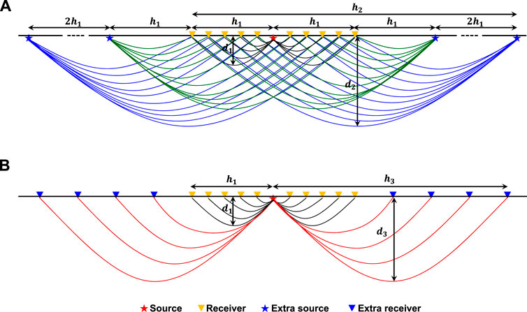
FIGURE 3. (A) Type-I modified geometry: extra sources are added into the normal geometry, that is, the red star source and yellow receivers. $h_1$ represents the maximum offset of the receiver array in the normal geometry part. The first extra source is set at a distance of $h_1$ to the nearest receiver. The interval of the rest of the extra sources is $2h_1$. (B) Type-II modified geometry: extra receivers are added into the normal geometry. The interval of the extra receivers is much sparser than the receivers of the normal geometry part. $h_2$ and $h_3$ indicate the maximum offset of the modified geometries for acquiring diving waves. $d_1$, $d_2$ and $d_3$ represent the maximum penetration depth of the diving waves.

The normal acquisition geometry part, that is, the red star source and yellow receivers in Figure 3, aims to acquire reflections and shallow diving waves. Its receiver interval is set about two times the interval of CMPs, which is related to the horizontal resolution. Usually, the receiver interval is small, for example, 20 m.

In Type-I modified geometry, the first extra source is set at a distance of $h_1$ to the nearest receiver, where $h_1$ indicates the maximum offset of the normal geometry part. The interval of the rest of the extra sources is two times $h_1$. With this setting, no source–receiver pair repeats the survey. This is demonstrated in Section 2.2. By contrast, in Type-II modified geometry, the extra receivers are installed along the extension line of the normal geometry. The extra receivers can be very sparsely positioned, which might lead to inaccurate shallow-region updates if this region is complex. This can be fixed by the diving waves that are recorded by dense receivers in the normal geometry. Therefore, the two parts of diving waves are complementary to each other for velocity building. The maximum offset of both modified geometries is set to acquire the diving waves from the targeted depth.

The Characteristics of the Modified Acquisition Geometries

The two types of modified geometries have different characteristics. Type-I modified geometry adds extra sources. The extra sources can be different from the source for acquiring reflections. In order to acquire long-distance traveling diving waves, the source energy, for example, the amount of dynamite or the number of seismic vibrators, can be increased to generate stronger and lower-frequency seismic signals. This modification increases the number of shots several times compared with the normal geometry. Thus, one cost-effective way is to apply seismic vibrators instead of dynamite.

By contrast, Type-II modified geometry adds extra receivers. It is inconvenient to achieve this acquisition geometry with cable-connected geophones due to the large offset. The most efficient way to implement this geometry is to use nodal seismometers, which do not need a cable for connection. However, this modified geometry needs to select appropriate sources that ensure diving waves reach the extra receivers. If the extra sources and receivers are the same as that used in the normal geometry, then the two modified geometries are in fact equivalent. Figure 4 illustrates this equivalence. Type-I geometry with only two extra sources shown in Figure 4A turns into Type-II geometry shown in Figure 4D. However, if the sources and receivers are different, the acquired data with the two geometries have different dynamics characteristics, for example, amplitude and frequency, but share similar travel time information. If the waveform is used for velocity building, match filtering can be used to remove the difference.

FIGURE 4

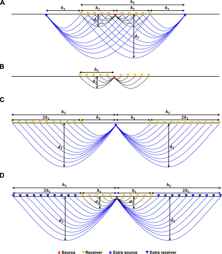
FIGURE 4. Equivalence between the two types of modified geometry. (A) Type-I modified geometry with only two extra sources added at two ends. This geometry is equal to the summation of (B) and (C). Consequently, Type-I geometry is equivalent to a Type-II geometry shown in (D). $h_1$ represents the maximum offset of the receiver array for the normal geometry part. It also denotes the offset of the extra sources to the nearest receivers. $h_2$ indicates the maximum offset generated by the extra sources. $d_1$ and $d_2$ represent the maximum penetration depth of the diving waves recorded by the receivers in the normal geometry and extra sources and receivers, respectively.

Workflow for Geometry Design

The improved geometries can be designed in three steps:

1) Determining the maximum offset and interval for acquiring reflections. Many studies have been done for this purpose. The general principle is that the maximum offset is set as about 1) 1.5 times the depth of targets, and the receiver interval is two times the expected horizontal resolution.

2) Determining the maximum offset for acquiring the diving waves. As a rule of the thumb, the maximum offset should be about 3–5 times the depth of the target. A more elegant way is to use ray tracing: building a background velocity model based on existing information about the survey area and then shooting rays into the velocity model to determine the offset that can receive the rays from the depth of the target.

3) Determining the interval of the extra receivers or sources. For Type-I geometry, the extra source interval is illustrated in Figure 3A: the first extra source is set at a distance of $h_1$ from its nearest receiver while the interval of rest of the extra sources is two times $h_1$. For Type-II geometry, an appropriate receiver array setting can achieve the condition that the rays should be dense in the shallow region but can be sparse in the deep region. This is because the width of the first Fresnel zone is narrow, that is, $w$ is small, in the shallow but wide, that is, $w$ is large, in the deep, which is illustrated in Figure 5. The shallow region is covered by the dense rays from the normal geometry for recording reflections so that the intervals of the extra receivers can be very sparse. However, it is hard to give exact criteria for the interval of the extra receivers and sources. One practical means is to do simulations with different parameters.

FIGURE 5

FIGURE 5. Schematic illustration of the first Fresnel zone for one source–receiver pair. $w$ indicates the width of the first Fresnel zone.

Examples

Synthetic Data Example

One synthetic model shown in Figure 6A is applied to demonstrate the two modified acquisition geometries for building velocity models and corresponding migration imaging. The initial velocity model is a 1D model shown in Figure 6B.

FIGURE 6

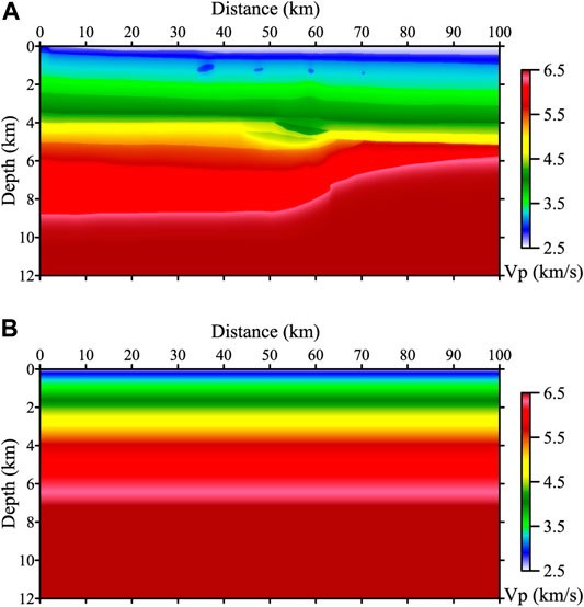
FIGURE 6. The velocity models for the numerical test. (A) The true velocity model. (B) The initial velocity model for velocity model building.

Since the deepest interface is at a depth of about 9 km, we set the maximum offset for acquiring reflections as 10 km, and choose a receiver interval of 20 m. The shot interval is set as 200 m. Then, we apply ray tracing on the initial model to determine the maximum offset for acquiring the diving wave that can penetrate to the depth of 9 km. The test indicates that an offset of 50 km is required. Consequently, Type-I modified geometry requires two extra sources at each side of the normal geometry. Type-II modified geometry needs extra receivers to cover 40-km extra offsets. Here, we set the extra receiver interval as 1 km. A 10-Hz Ricker wavelet is used as the source wavelet. One shot record is shown in Figure 7.

FIGURE 7

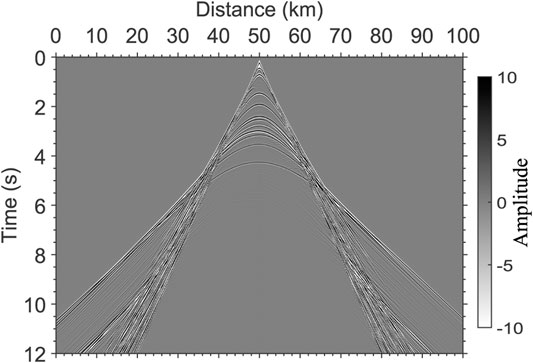
FIGURE 7. One shot record acquired in the middle of the model. The maximum offset is 50 km.

We picked up the first breaks from the records and then used travel time tomography to recover the velocity model. First, we inverted the first-arrival travel time of the record from the normal geometry, which has a maximum offset of 10 km. The recovered velocity model and its ray density map are shown in Figure 8. As can be seen, the inversion only recovers the top 1 km of the model because the diving wave only penetrates such a depth, which is indicated by the ray coverage area in Figure 8B.

FIGURE 8

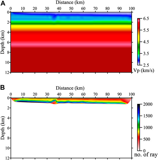
FIGURE 8. The inverted velocity model (A) with a maximum offset of 10 km and (B) its ray density map.

We then inverted the first breaks of the dataset from Type-I geometry. The recovered model is depicted in Figure 9A. As can be seen, it recovers the background velocity of the true model and the shallow low-velocity anomalies, correctly. As analyzed in the previous section, Type-I geometry is equivalent to Type-II geometry with a trace interval of 20 m for extra receivers. As a result, this recovered model can be treated as that of Type-I geometry with the densest trace interval for the extra receivers.

FIGURE 9

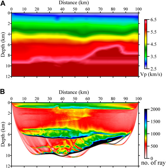
FIGURE 9. The inverted velocity model (A) with Type-I modified geometry and (B) its ray density map. The maximum offset of the normal geometry part is 10 km. Two extra sources were excited at both sides of the receiver array.

Next, we inverted the first breaks of the dataset from Type-II geometry, in which the receiver interval is 1 km for the extra receivers. The recovered model is shown in Figure 10A. Compared with the model from Type-I geometry, they share a similar background trend. This implies that the extra receivers can be very sparse. We also carried out tests with smaller intervals for the extra receivers, for example, 100 and 500 m. Results show that denser extra receivers give slightly better details but share a similar background velocity trend.

FIGURE 10

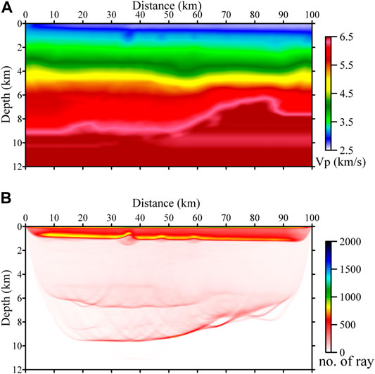
FIGURE 10. The inverted velocity model (A) with Type-II modified geometry and (B) its ray density map. The maximum offset of the normal geometry part is 10 km. The interval of extra receivers is 1 km. The maximum offset of the modified geometry is 50 km.

To investigate the significance of the diving waves in the normal geometry, that is, the first 10-km offset in this example, we repeated the inversion but without the first 10-km offset data. The result is shown in Figure 11A. Compared with the model shown in Figures 9A, 10A, it is clear that the shallow part of the model, that is, top 1 km part, was not recovered correctly. This means that the diving wave recorded by the normal geometry is important for recovering the shallow region of the model.

FIGURE 11

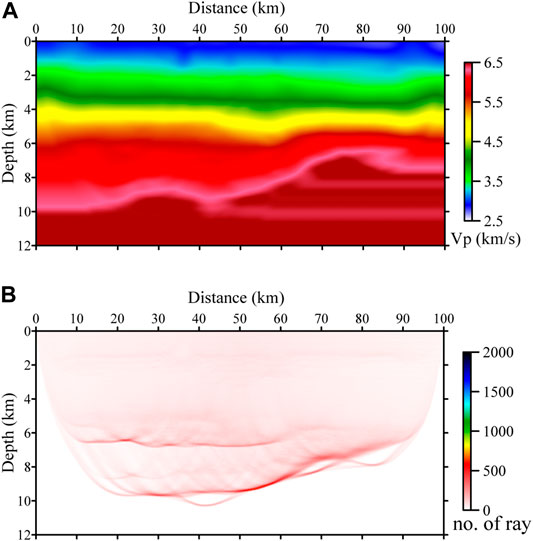
FIGURE 11. The inverted velocity model (A) with Type-II modified geometry but without the 10-km receiver arrays in the normal geometry and (B) its ray density map. The interval of extra receivers is 1 km. The maximum offset of the modified geometry is 50 km.

To verify the accuracy of the recovered velocity models, we carried out Kirchhoff pre-stack depth migration (PSDM). These migration images are shown in Figure 12. A corresponding common image gather (CIG) extracted at a distance of 50 km is depicted in Figure 13. As can be seen, both modified geometries acquired adequate diving waves resulting in successfully recovering the background velocity. In addition, the diving waves recorded by the normal geometry are crucial for the shallow region recovery.

FIGURE 12

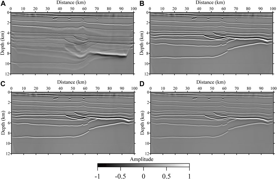
FIGURE 12. Kirchhoff PSDM profiles: migration velocity shown in (A) Figure 8A, (B) Figure 9A, (C) Figure 10A, and (D) Figure 11A.

FIGURE 13

FIGURE 13. CIG profiles at a distance of 50 km. (A–D) corresponds to (A–D) in Figure 12, respectively.

Field Data Example

To validate our concept, we applied Type-II geometry in a seismic survey in East China for constructing the velocity model of a sedimentary basin. The conventional acquisition geometry utilizes a split spread. The shot interval is 250 m. The maximum offset is 4.7 km with a receiver interval of 6.25 m. The nodal seismometers were deployed every 3 km along the whole 21-km survey line, which can give a maximum penetration depth of about 5 km.

We carried out the first-arrival tomography to recover the background velocity, which is shown in Figure 14B. The first-arrival data from both conventional geometry and the sparse nodal seismometers were used in the tomography. The ray density map is shown in Figure 14C. Note that the small receiver interval in the conventional geometry part provides dense ray coverage in the shallow region, which is crucial for correctly recovering the region’s velocity. The initial velocity model is the stacking velocity (Figure 14A) from the contractor company. The stacking velocity is created by depth conversion from the NMO velocity through the semblance velocity analysis. Although the semblance velocity analysis is not the cutting-edge method of velocity model building, the stacking velocity is still widely used in seismic exploration as a good initial estimation of the underground velocity.

FIGURE 14

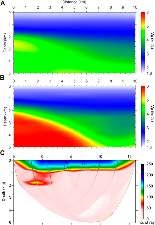
FIGURE 14. Velocity models: (A) the stacking velocity using reflection data from the normal geometry and (B) first-arrival tomographic velocity with Type-II geometry. (C) The ray density map.

It shows that the tomographic velocity model constructed by our Type-II geometry contains more details in deep regions than the stacking velocity model constructed by semblance velocity analysis. The tomographic velocity has higher values than the stacking velocity at the bottom of the sedimentary basin. Those differences in the velocity models lead to a noticeable improvement in the migration results shown in Figure 15. The migration used the reflection data recorded with the conventional geometry. The migration profile using the tomographic velocity shows better continuity of reflection events (green arrows) and convergence of faults (red arrows) than that using the stacking velocity. The results indicate that our proposed modified geometry through the combination of nodal seismometers and the conventional seismic cable shall be suitable for constructing a deep velocity model.

FIGURE 15

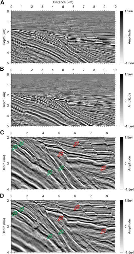
FIGURE 15. The Kirchhoff PSDM migration images with (A) the stacking velocity and (B) the tomographic velocity. (C) and (D) are the enlarged view of the migration images shown in (A,B), respectively. The red arrows indicate better-focused faults. The green arrows point out better-imaged reflectors.

Discussion

In this article, we only analyzed the modified geometries for a 2D seismic survey. However, it is straightforward to extend the two types of modified geometries to a 3D seismic survey. Extra sources and extra receivers were deployed around the 2D receiver arrays. For Type-I geometry, extra sources were deployed not only along inlines but also in crosslines; consequently, the number of extra sources increases significantly compared to that for the 2D seismic survey. According to the analysis before, Type-I geometry is equivalent to the densest receiver interval in Type-II geometry. Thus, two means can mitigate this issue: the first one is to reduce the extra source number; the second one is to use a cost-effective seismic source, for example seismic vibrators. For Type-II geometry, the most cost-effective way is to use nodal seismometers for recording the large-offset diving waves. As demonstrated by the field data example, an interval of 3 km still delivered a good velocity model. Thus, one nodal seismometer can cover a 9 km² area. The modified geometries, therefore, are practical for a large 3D seismic survey.

Conclusion

Building accurate seismic velocity models is the key for seismic migration imaging. Current seismic surveys are mainly designed for acquiring reflections. Due to limited offsets, the recorded diving waves in a normal geometry have limited penetration depth. Consequently, the velocity model building relies on reflections. The low S/N ratio and incomplete information of reflection data prevent successful velocity model building. Building velocity models with diving waves can tackle this problem. We, therefore, propose two types of modified geometries to record the diving waves at a large offset, which can penetrate to a large depth. Type-I geometry adds extra sources along the extension line of the receiver array, whereas Type-II geometry deploys extra receivers along the extension line. Analysis shows that the two geometries have different characteristics. Seismic vibrators are a cost-effective choice for Type-I geometry, whereas nodal seismometers are a convenient choice for Type-II geometry. We also provide the workflow for designing the geometries. Both synthetic and field data examples demonstrate that the proposed improved acquisition geometries can record the diving waves from the deep subsurface. Their first arrivals are used to successfully build velocity models that are enough to imaging deep targets. By contrast, the diving wave from conventional geometry only recovers the shallow velocity.

Data Availability Statement

The original contributions presented in the study are included in the article/Supplementary Material, further inquiries can be directed to the corresponding authors.

Author Contributions

GY, ZZ, SW, and NL invented the idea of the article. NL, JZ, DW, and XL carried out the test and draw the figures. GY drafted the article. All authors reviewed the article.

Funding

This work was partially supported by the National Key R&D Program of China (grant no. 2018YFA0702502), the National Natural Science Foundation of China (grant nos 41974142 and 42074129), Fundamental Research Funds for the Central Universities (grant nos 201964017 and 202072002), Science Foundation of China University of Petroleum (Beijing) (grant no 2462020YXZZ005), and State Laboratory of Petroleum Resource and Prospecting (grant no. PRP/indep-4-2012).

Conflict of Interest

The authors declare that the research was conducted in the absence of any commercial or financial relationships that could be construed as a potential conflict of interest.

Publisher’s Note

All claims expressed in this article are solely those of the authors and do not necessarily represent those of their affiliated organizations, or those of the publisher, the editors, and the reviewers. Any product that may be evaluated in this article, or claim that may be made by its manufacturer, is not guaranteed or endorsed by the publisher.

References

Berkhout, A. J. (1980). Seismic Migration Imaging of Acoustic Energy by Wave Field Extrapolation. Newyork: Elsevier.

Google Scholar

Dellinger, J., Ross, A., Meaux, D., Brenders, A., Gesoff, G., Etgen, J., et al. (2016). “Wolfspar, an "FWI-Friendly" Ultralow-Frequency marine Seismic Source,” in SEG Technical Program Expanded Abstracts 2016 (October 17, 2016; Dallas, Texas). doi:10.1190/segam2016-13762702.1

CrossRef Full Text | Google Scholar

Kosloff, D., Sherwood, J., Koren, Z., Machet, E., and Falkovitz, Y. (1996). Velocity and Interface Depth Determination by Tomography of Depth Migrated Gathers. Geophysics 61 (5), 1511–1523. doi:10.1190/1.1444076

CrossRef Full Text | Google Scholar

Lewis, W., Amazonas, D., Vigh, D., and Coates, R. (2014). “Geologically Constrained Full-Waveform Inversion Using an Anisotropic Diffusion Based Regularization Scheme: Application to a 3D Offshore Brazil Dataset,” in SEG Technical Program Expanded Abstracts 2014 (October 28, 2014. Denver, Colorado). doi:10.1190/segam2014-1174.1

CrossRef Full Text | Google Scholar

Li, W., Liu, Y.-K., Chen, Y., Liu, B.-J., and Feng, S.-Y. (2021). Active Source Seismic Imaging on Near-Surface Granite Body: Case Study of Siting a Geological Disposal Repository for High-Level Radioactive Nuclear Waste. Pet. Sci. 18, 742–757. doi:10.1007/s12182-021-00569-8

CrossRef Full Text | Google Scholar

Liu, F., Zhang, G., Morton, S. A., and Leveille, J. P. (2011). An Effective Imaging Condition for Reverse-Time Migration Using Wavefield Decomposition. Geophysics 76 (1), S29–S39. doi:10.1190/1.3533914

CrossRef Full Text | Google Scholar

Shen, X., Ahmed, I., Brenders, A., Dellinger, J., Etgen, J., and Michell, S. (2018). Full-waveform Inversion: The Next Leap Forward in Subsalt Imaging. Leading Edge 37 (1), 67b1–67b6. doi:10.1190/tle37010067b1.1

CrossRef Full Text | Google Scholar

Sheriff, R. E. (2002). Encyclopedic Dictionary of Applied Geophysics. 4th Ed. Oklahoma: Society of Exploration Geophysicists. doi:10.1190/1.9781560802969

CrossRef Full Text | Google Scholar

Sherwood, J., Chen, K. C., and Wood, M. (1986). “Depths and Interval Velocities from Seismic Reflection Data for Low Relief Structures,” in SEG Technical Program Expanded Abstracts 1986 (November 5, 1986; Houston, Texas). doi:10.1190/1.1892903

CrossRef Full Text | Google Scholar

Tarantola, A. (1984). Inversion of Seismic Reflection Data in the Acoustic Approximation. Geophysics 49 (8), 1259–1266. doi:10.1190/1.1441754

CrossRef Full Text | Google Scholar

Virieux, J., and Operto, S. (2009). An Overview of Full-Waveform Inversion in Exploration Geophysics. Geophysics 74 (6), WCC1–WCC26. doi:10.1190/1.3238367

CrossRef Full Text | Google Scholar

Warner, M., Ratcliffe, A., Nangoo, T., Morgan, J., Umpleby, A., Shah, N., et al. (2013). Anisotropic 3D Full-Waveform Inversion. Geophysics 78 (2), R59–R80. doi:10.1190/geo2012-0338.1

CrossRef Full Text | Google Scholar

Wu, Z., and Alkhalifah, T. (2015). Simultaneous Inversion of the Background Velocity and the Perturbation in Full-Waveform Inversion. Geophysics 80 (6), R317–R329. doi:10.1190/geo2014-0365.1

CrossRef Full Text | Google Scholar

Xu, S., Wang, D., Chen, F., Lambaré, G., and Zhang, Y. (2012). “Inversion on Reflected Seismic Wave,” in SEG Technical Program Expanded Abstracts 2012. November 6, 2012. Las Vegas, Nevada. doi:10.1190/segam2012-1473.1

CrossRef Full Text | Google Scholar

Yao, G., and Wu, D. (2017). Reflection Full Waveform Inversion. Sci. China Earth Sci. 60 (10), 1783–1794. doi:10.1007/s11430-016-9091-9

CrossRef Full Text | Google Scholar

Yao, G., da Silva, N. V., and Wu, D. (2019). Reflection-Waveform Inversion Regularized with Structure-Oriented Smoothing Shaping. Pure Appl. Geophys. 176 (12), 5315–5335. doi:10.1007/s00024-019-02265-6

CrossRef Full Text | Google Scholar

Yao, G., Wu, D., and Wang, S.-X. (2020). A Review on Reflection-Waveform Inversion. Pet. Sci. 17 (2), 334–351. doi:10.1007/s12182-020-00431-3

CrossRef Full Text | Google Scholar

Yilmaz, Ö. (2001). Seismic Data Analysis: Processing, Inversion, and Interpretation of Seismic Data. Oklahoma: Society of Exploration Geophysicists. doi:10.1190/1.9781560801580

CrossRef Full Text | Google Scholar

Zhang, Y., and Sun, J. (2008). “Practical Issues of Reverse Time Migration - True-Amplitude Gathers, Noise Removal and Harmonic-Source Encoding,” in 70th EAGE Conference & Exhibition - Rome (June 10, 2008. Rome). doi:10.3997/2214-4609.20147708

CrossRef Full Text | Google Scholar

Zhang, Z., Mei, J., Lin, F., Huang, R., and Wang, P. (2018). “Correcting for Salt Misinterpretation with Full-Waveform Inversion,” in SEG Technical Program Expanded Abstracts 2018 (October 16, 2018. Anaheim California). doi:10.1190/segam2018-2997711.1

CrossRef Full Text | Google Scholar

Zhou, W., Brossier, R., Operto, S., and Virieux, J. (2015). Full Waveform Inversion of Diving & Reflected Waves for Velocity Model Building with Impedance Inversion Based on Scale Separation. Geophys. J. Int. 202 (3), 1535–1554. doi:10.1093/gji/ggv228

CrossRef Full Text | Google Scholar

Zhou, H. w. (2003). Multiscale Traveltime Tomography. Geophysics 68 (5), 1639–1649. doi:10.1190/1.1620638

CrossRef Full Text | Google Scholar