
94% of researchers rate our articles as excellent or good
Learn more about the work of our research integrity team to safeguard the quality of each article we publish.
Find out more
ORIGINAL RESEARCH article
Front. Earth Sci., 05 July 2022
Sec. Quaternary Science, Geomorphology and Paleoenvironment
Volume 10 - 2022 | https://doi.org/10.3389/feart.2022.848652
This article is part of the Research TopicGlaciation and Climate Change in the Andean CordilleraView all 17 articles
 Brittany N. Price1*
 Nathan D. Stansell1
 Alfonso Fernández2
 Joseph M. Licciardi3
 Alia J. Lesnek3,4
 Ariel Muñoz5,6,7
 Mary K. Sorensen1
 Edilia Jaque Castillo8
 Tal Shutkin9,10Isabella Ciocca2
 Ianire Galilea8
The development of robust chronologies of Neoglaciation from individual glaciers throughout the high-altitude Andes can provide fundamental knowledge of influences such as regional temperature and precipitation variability, and aid in predicting future changes in the Andean climate system. However, records of Late Holocene glaciation from the Central Chilean Andes are sparse, and often poorly constrained. Here, we present 36Cl surface exposure ages, dendrochronologic constraints, and glacial mass balance modeling simulations of Late Holocene glacier fluctuations in the Central-South Chilean Andes. A series of concentric moraine ridges were identified on Monte Sierra Nevada (38°S), where exposure dating of basaltic boulders was used to establish a chronology of ice recession. We infer that moraine abandonment of the most distal ridge in the valley commenced by ∼4.2 ka, and was followed by glacier margin retreat to an up-valley position. Exposure ages of the oldest Late Holocene boulders (∼2.5–0.8 ka) along the marginal extents of the moraine complex indicate fluctuations of the glacier terminus prior to ∼0.65 ka. A final expansion of the ice margin reoccupied the position of the 4.2 ka moraine, with abatement from the outermost composite moraine occurring by ∼0.70 ka, as constrained by tree-ring data from live Araucaria araucana trees. Finally, a series of nested moraines dating to ∼0.45–0.30 ka, formed from a pulsed ice recession during the latest Holocene when the lower reaches of the glacial snout was most likely debris mantled. A distributed temperature index model combined with a glacier flow model was used to quantify an envelope of possible climatic conditions of Late Holocene glaciation. The glacial modeling results suggest conditions were ∼1.5°C colder and 20% wetter during peak Neoglaciation relative to modern conditions. These records also suggest a near-coeval record of Late Holocene climate variability between the middle and high southern latitudes. Furthermore, this study presents some of the youngest 36Cl exposure ages reported for moraines in the Andes, further supporting this method as a valuable geochronologic tool for assessing Late Holocene landscape development.
The Central-South Chilean (CSCh, Table 1) Andes (∼37.5°S) marks a critical climatic and geographic boundary between the low and high latitudes (Muñoz et al., 2016), thus studying glacial fluctuations in this region can provide information about past inter-hemispheric oceanic and atmospheric dynamics (Liu and Yang, 2003). To the south, glacial mass balances in the Northern Patagonian Andes are largely dominated by the strength of Pacific Ocean westerlies, El Niño Southern Oscillation (ENSO), and the South Pacific Subtropical High (SPSH) (Aravena and Luckman, 2009; Garreaud et al., 2009; Garreaud et al., 2013). Likewise, the Southern Annular Mode (SAM) affects the position and intensity of the westerlies, summer temperatures, and rainfall distribution (Gillett et al., 2006; Reynhout et al., 2019). Disentangling these complex systems is critical for our ability to predict future changes in the Andean environment and global climate system in response to natural and anthropogenic forcings. Our research aims to evaluate the climatic conditions driving glacial growth and decay in the CSCh Andes over the Late Holocene, and assess whether discreet leads and lags in the Andean cryosphere system are discernable regionally over the Neoglacial period.
TABLE 1. Abbreviations used in manuscript.
Glacial melt is an important source of water in CSCh, so properly understanding the conditions and locations of glacier survival under future warming scenarios is pivotal to mitigating current water usages for sustainability (Huss and Fischer, 2016; Barcaza et al., 2017; Racoviteanu et al., 2021). In this context, it is unclear how individual glaciers might respond to localized climatic effects vs. more regional or synoptic-scale processes (Rupper and Roe, 2008), as future climate change scenarios will not impact all regions of the Andes synchronously, or at the same rate or magnitude. Furthermore, other landscape-specific questions have yet to be addressed, such as the extent of debris coverage on regional glaciers in the recent past, an important factor for understanding mountain water storage.
Our ability to link Chilean glacial variability and specific environmental forcings will be improved with a robust chronology of past events. At present, individual records are often broadly bracketed by both minimum and maximum ages, resulting in chronologies that lack the resolution necessary to fully decern the local stratigraphy. By integrating surface exposure dating and dendrochronology (Harrison et al., 2008; Nimick et al., 2016), we aim to better constrain the timing of Late Holocene glacial fluctuations from CSCh.
Various chronologies of glacial advances have been proposed to reflect the datasets gathered from southernmost South America. For example, Mercer (1976) originally proposed three distinct Neoglacial events in the Chilean Andes, while Aniya (2013) posited five Neoglacial events over the same interval, with subtle differences in the timing of glacial advances and retreat. Nevertheless, glacier fluctuations in the CSCh Andes and northern Patagonia still lack detailed regional records to constrain large scale recessional timing during Neoglaciation, and particularly the Late Holocene. A more recent examination of glacial records from northern Patagonia dates the greatest ice readvances from the Late Holocene to between 2–1 ka and 0.5–0.2 ka, with the largest overall advances since the mid-Holocene occurring at ∼5 ka (Davies et al., 2020).
Recent developments in cosmogenic dating now allow direct age determination on Neoglacial moraine boulders, including the Southern Hemisphere expression of the LIA, defined as 0.67–0.17 ka (García-Ruiz et al., 2014; Solomina et al., 2015; Jomelli et al., 2016). Exposure ages this young have more commonly been derived from 10Be measurements on silica-rich rocks (Licciardi et al., 2009; Schürch et al., 2016; Dong et al., 2017; Biette et al., 2021), and until recently dating the basalt-rich rocks in the CSCh Andes has been seldomly attempted. These basalts often lack well-developed phenocrysts (e.g., feldspars) necessary for analyzing 36Cl in mineral separates, which can minimize complexities and uncertainties in 36Cl production and exposure age interpretations (Wirsig et al., 2016). Currently, only a few studies have applied similar methods to date moraine boulders in volcanic landscapes (e.g., Alcalá-Reygosa et al., 2018), largely because of 36Cl production systematics that yield high uncertainties in Cl-rich rocks (e.g., Palacios et al., 2017). Despite challenges associated with 36Cl surface exposure dating, this cosmogenic nuclide is well-suited for lithologies lacking quartz, and allows for exposure dating of moraine boulders that in some cases were emplaced only hundreds of years ago (Jomelli et al., 2016; Jomelli et al., 2017; Charton et al., 2021a; Verfaillie et al., 2021).
Glacial studies in the Chilean Andes have also been hindered by a lack of physically-based models that test a range of climate drivers (Pellicciotti et al., 2014). As such, our knowledge of fundamental influences like temperature and precipitation changes on individual glaciers and ice caps throughout the Andes remain minimally constrained. Moreover, different modeling approaches produce a diverse range of outputs at varying resolutions, making it difficult to converge on a standardized approach for interpreting past glacial variability (Fernández and Mark, 2016). Nevertheless, coupling local station data with temperature index models produces first-order estimates of glacial sensitivity to climate change (Hock and Holmgren, 2005), including paleo-climate scenarios (Kull and Grosjean, 2000). Testing and deploying a physically-based glacier mass balance model provides a tool for addressing outstanding questions relating to the timing and causes of Late Holocene climate change. Climatic conditions during Late Holocene glacial advances are assessed to have been cold and wet, corresponding to a negative SAM phase (Moreno et al., 2018), but the magnitude of these temperature and precipitation changes have yet to be quantified for specific regions of the Andes.
Here we present a new glacial chronology using independently derived tree-ring data combined with 36Cl ages on glacial boulders from a cirque valley atop Monte Sierra Nevada, Chile (38°34′56″ S, 71°34′47″ W) (Figure 1). Located at the southernmost expression of an area (31–38°S) categorized as hosting warm- and wet-based glaciers, the glacial mass balance here should be sensitive to both temperature and precipitation changes (Sagredo and Lowell, 2012). This chronology is coupled with the Hock (1999) distributed temperature index model (DETIM), establishing a range of possible precipitation and temperature values at the time of moraine abandonment using proxy and modeled data.

FIGURE 1. Map of South America with Chile (beige with brown outline). Relative positions of the winds associated with the dominant precipitation bearing South Pacific Subtropical High (SPSH), and Southern Westerly Wind Belt (SWWB) during the Austral summer months are indicated with black arrows. Major oceanic currents near the study site (Antarctic Circumpolar Current, Peru-Chile Current and Cape Horn Current) are indicated with blue arrows. Inset box shows the proximity of the identified modern climatic transition zone of ∼37.5°S (Muñoz et al., 2016) to the nearby Araucanía region of Chile (filled in red). A yellow star identifies the location of Monte Sierra Nevada (∼38°S), and the location of the Temuco weather station used for the modeling analysis is represented by a purple circle.
Monte Sierra Nevada stands at 2,527 m above sea level (a.s.l.), with ice capping the highest peaks and extending partially down several east-facing cirque valleys (Figure 2). The site is located to the west of the Cordillera Principal, which is made up of the granitoid North Patagonia Batholith (The Cura-Mallin Formation) of Cretaceous and Miocene age (Glodny et al., 2006). Pleistocene and Holocene volcanoes (e.g., Llaima, Lonquimay, Sierra Nevada, and Tolhuaca) make up the active volcanic arc of the Cordillera Principal that formed on the eroded, and relatively flat-lying Miocene-aged rocks (Muñoz et al., 2011). Regionally, this southern volcanic zone is predominantly composed of basalts and basaltic andesites (Hickey et al., 1986; Ferguson et al., 1992; Muñoz et al., 2011). Additionally, these active Holocene volcanos might have deposited volcanic ash on glaciated terrain, potentially affecting glaciers’ response to climate changes by two competing effects associated with debris thickness and temperature: insulation from incoming energy or enhancement of ablation (Davies and Glasser, 2012).
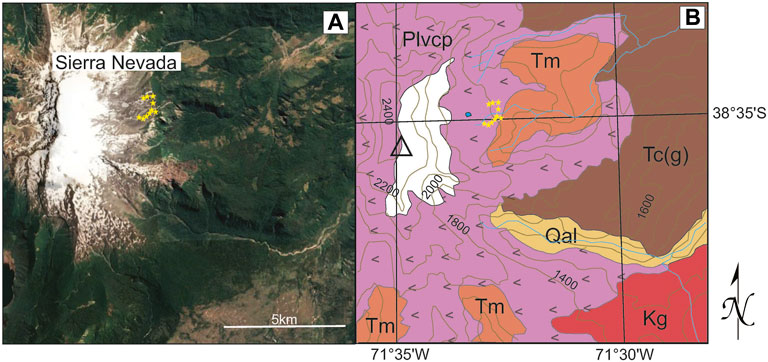
FIGURE 2. Panel (A) Google Earth map of Monte Sierra Nevada and surrounding area with sample locations marked by yellow stars. Panel (B) Geologic map, modified from Muñoz et al. (2011). Qal—Quaternary alluvium, Plvcp—Upper Pleistocene-Holocene volcanic rocks, Tc—Miocene Cura-Mallin Formation, Tm—Miocene Melipeuco Plutonic Group, Kg—Cretaceous Galletué Plutonic Group.
In our study area, there are a total of five morainal loops along the valley floor over a distance of ∼350 m (Figure 3). Mapped moraines exhibit variable effects of weathering and erosion suggesting relative age differences. We number each moraine, starting with the oldest and most distal from the current glacier front (M1), progressing westward to the youngest, most ice-proximal moraine (M5) (Figure 3). Visually, moraine M2 is the largest and most intact of the moraine complex, while moraine M1 is the sole moraine in the valley with observed soil development, and exhibits a subtle dual-crest to the south of the field site. On the ice-proximal side of moraine M5 chaotic hummocks are observed, with glacial scree deposits further up valley (Figure 4). Additionally, several striated boulders and roches moutonnées are observed, both within and outside of the moraine complex.
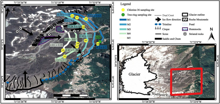
FIGURE 3. Panel (A) Google Earth image of the Monte Sierra Nevada field site, with the modern glacier outlined in black and the moraine complex outlined in red. Panel (B) Ariel photograph of the field site as delineated by red box in panel A. Map identifies glacial moraines (M1-M5), locations of samples taken for 36Cl (yellow circles with abbreviated sample number) and tree ring (green circle) dating. 36Cl ages are reported in thousand years before present with internal uncertainty. Probable ice flow directions are represented by black arrows based on observed striated rock surfaces (white circles). Trimline along the southern ridge of the valley is marked (blue dashed line), as well as the saddle and chute (black line).
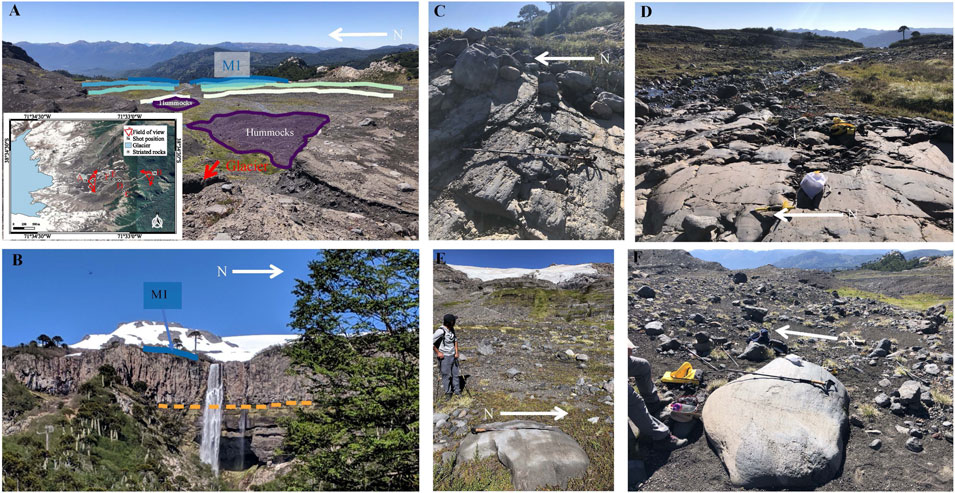
FIGURE 4. Photographs of the Monte Sierra Nevada field site. Panel (A) Facing east the hummocky areas of the field site are outlined on the glacier proximal side of moraine M5 (purple). Panel (B) Facing west with the modern glacier in the background and contact between Pleistocene and Miocene volcanic rocks (orange dashed line) in the foreground behind waterfall. The cliff marks the limit of preserved Neoglacial moraine boulders, with moraine M1 (blue line) denoted to the south of the waterfall. The combined effects of topoclimatic constrains (i.e., lower elevations, seasonally constrained snow accumulation) make the existence of large glaciers in CSCh unlikely, as Neoglacial landforms are generally indistinguishable below this abrupt change in elevation. A grove of A. araucana trees is pictured to the south of the waterfall in the foreground. Panel (C–F) Striated boulders and roches moutonnées used for directional data to infer paleo-flowlines of the glacier. Inset map in panel A shows the location of each field picture, with letters corresponding to each panel.
The geomorphology of Monte Sierra Nevada yields information on the relative timing of glacial landform development due to the stratigraphy observed in the valley. For example, the distal end of the valley is truncated by a steep cliff at the contact between the relatively flat-lying Pleistocene volcanic layers and the underlying Miocene plutonic rocks (Figure 4). The steep topography below this contact likely precludes the establishment of moraines from glacial advances that were more extensive than the presumed Late Holocene moraines that end just before a steep drop in topography to the valley below. On Monte Sierra Nevada, moraines are generally limited to elevations between ∼1,703 and 1,722 m a.s.l (Table 2) and the moraines have since been bifurcated by Holocene stream development.
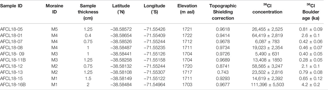
TABLE 2. Sample information used in the calculation of the36Cl boulder age expressed with internal uncertainty, calculated with a rock formation age of 130 ka using a developmental version of the CRONUS-Earth36Cl calculator (Balco et al., 2008; http://stoneage.ice-d.org/math/Cl36/v3/v3_Cl36_age_in.html) and LSDn scaling. The ICE-D calibration datasets used can be found at http://calibration.ice-d.org/allcds.
Directly south of the valley with the mapped moraine complex is a ridge separating it from the adjacent, topographically higher valley (Figure 3). On the ridge separating the two valleys is a well-defined saddle and chute, both of which are currently ice free. Along this same ridge is a trimline indicating the most recent highest extent of ice thickness in the valley. This trimline extends down valley intersecting moraine M1, as well as up valley past the saddle and chute towards the mountain’s peak. The chute exhibits a cross-cutting relationship with the trimline, having eroded any recognizable lateral features. Notable talus deposits are identifiable along the northern and southern valley walls, particularly below the trimline and along the chute. The modern glacial ice cap on Monte Sierra Nevada extends into the uppermost reaches of both valleys.
Central Chile has a Mediterranean-type climate with mild, wet winters and dry, hot summers. The modern climate is largely modulated by Pacific and Southern Ocean processes, resulting in a strong seasonality of precipitation south of ∼35°. winter storms dominate here, bringing ∼2,000 mm of annual rainfall to the region (Sinclair, 1996; Garreaud et al., 2009). However, Monte Sierra Nevada (38°S) is located near what is considered to be a transition zone between Mediterranean-subtropical and temperate-humid climatic zones, identified at ∼37.5°S (Figure 1; Muñoz et al., 2016). Precipitation at this location is therefore impacted by shifts in the subtropical South Pacific Subtropical High (SPSH) and extratropical Southern Westerly Wind Belt (SWWB) year-round (Miller, 1976; Espinoza et al., 2020).
Glaciers in CSCh predominantly receive precipitation sourced from the Pacific Ocean due to the moisture barrier produced by the Andes mountains (Montecinos and Aceituno, 2003). Isotopic analyses of precipitation suggest that Atlantic-derived moisture rarely penetrates through to the western flanks of the Andes (Hoke et al., 2013). While regionally both the height and width of the CSCh Andes are smaller in comparison to the Northern Cordillera, orographic precipitation leads to continental precipitation values that are up to three times larger than corresponding oceanic amounts (Garreaud et al., 2009).
In Central Chile the SPSH typically fluctuates between ∼25 and 35°S and delivers moist air masses to the western slope of the Andes (Ancapichún and Garcés-Vargas, 2015). Active year-round, the position of the SPSH is modulated by the Bolivian High, which migrates northward during the austral winter (May-August) as the jet stream moves equatorward. This increase in winter storm tracks drives midlatitude precipitation along the central Chilean coast (Sinclair, 1996; Lamy et al., 2001; Garreaud et al., 2009; Espinoza, et al., 2020). From February-April the SPSH shifts south, resulting in increased precipitation off the coast of CSCh (∼37°S) (Ancapichún and Garcés-Vargas, 2015). This hydrologic regime results in an enhanced probability of aridity in CSCh, as streamflow peaks in winter due to rainfall and again in late spring as seasonal snow melts in the mountains.
The regional climate in the CSCh Andes is also affected by the Antarctic Circumpolar Current (ACC). The ACC splits as it approaches the western coast of South America between ∼40 and 45°S (Boltovskoy, 1976; Villalba et al., 2012), with the Peru-Chile Current flowing north and the Cape Horn Current flowing south (Lamy et al., 2007). The Peru-Chile Current transports cold, low-saline waters equatorward (Strub, 1998), with seasonal changes in upwelling driven by the position and intensity of the SPSH (Garreaud et al., 2009; Ancapichún and Garcés-Vargas, 2015). The SPSH is thus one of the dominant controls on sea surface temperatures (SSTs) associated with the Peru-Chile Current, with the ability to increase upwelling and offshore Ekman transport. The position of the ACC also results in strong winds directed at the coast, in the form of the SWWB. Situated between the subtropical anticyclone and subpolar cyclonic air masses, these westerlies bring strong winds and abundant precipitation to CSCh and the adjacent northern Patagonian Andes, intersecting the western coast of South America between 40°S-55°S (Bertrand et al., 2014). During Austral summer the SWWB strengthens, contracts, and shifts to the southern extent of its range in response to southern-ocean processes, while during the winter months the SWWB weakens and expands both poleward and towards the equator (Bentley et al., 2009). Comparatively, the SWWB is stronger than the storm tracks associated with the SPSH at the study location, as it is confined to a smaller latitudinal range and more directly affects regional precipitation.
Located in the transition zone between Mediterranean and temperate climates, both ENSO and SAM play important roles in driving changes in temperature and moisture availability to Monte Sierra Nevada. ENSO is characterized by shifting oceanic-atmospheric conditions in the tropical Pacific, the effects of which are superimposed on the climate system of CSCh. El Niño (La Niña) years are associated with a weakening (strengthening) of the Peru-Chile Current, due to a reduction in the east-west pressure gradient (Montecinos and Aceituno, 2003), forcing a weaker SPSH into more northerly position (Villalba, 1994). This northward displacement of the SPSH reduces moisture availability in CSCh. When SSTs are lower the high-pressure system strengthens, and westerly trade winds intensify in response (Bertrand et al., 2014). In the northern portion of the transition zone (35–40°S), ENSO is characterized as having a stronger influence on the SPSH (Rutllant and Fuenzalida, 1991), whereas south of ∼40°S interannual precipitation driven by the SWWB is heavily modulated by the strength/phase of the SAM (Aravena and Luckman, 2009; Garreaud et al., 2009; Villalba et al., 2012).
The SAM is measured by changes in sea-surface pressure between the mid- and high-latitudes (Villalba et al., 2012; Ancapichún and Garcés-Vargas, 2015). Both the strength and position of the SWWB is dictated by SSTs, and sea surface pressure gradients associated with the ACC and the Southern Ocean, specifically the SAM (Gillett et al., 2006; Reynhout et al., 2019). Enhancement of precipitation in Patagonia south of ∼55°S is predominantly driven by a southern displacement of the SWWB, subsequently resulting in decreased precipitation around 38–43°S. During negative (positive) phases of the SAM the SWWB shifts equatorward (poleward), resulting in more humid (arid) conditions in CSCh (Garreaud et al., 2009; Bertrand et al., 2014; Muñoz et al., 2016).
Proxy paleo-climate evidence suggests that Late Holocene glacial variability in the northern Patagonia Ice Field was driven by both precipitation and temperature (Bertrand et al., 2012). A tree-ring reconstruction of summer temperatures from northern Patagonia suggests there was a cold interval from ∼1.1 to 0.95 ka, followed by warming until ∼0.77 ka and another phase of cool and wet conditions peaking between ∼0.68 and 0.38 ka (Villalba, 1994). Proxy paleoclimate records also suggest that from ∼0.65 ka until the last century was the wettest interval of the last ∼5,000 years in the southern Chilean Andes (Moreno et al., 2009). Moreno et al. (2018) strengthened this analysis, and documented that regional glacial advances in the southern Patagonia Ice Field were forced from negative SAM phases (cold and wet), that were modulated on regional scales by the position and intensity of the SWWB. Recently, Davies et al. (2020) compiled geomorphic evidence and recalibrated chronological data from dozens of studies assessing fluctuations of the Patagonian Ice Sheet from 35 ka to the present. Records detailing the Late Holocene from 41°S to 52°S noted climatic conditions alternated between cold/wet and warm/dry on centennial time scales (Elbert et al., 2013; Álvarez et al., 2015; Moreno and Videla, 2016; Moreno et al., 2018; Davies et al., 2020). Well-defined Late Holocene moraines are apparent regionally (Glasser et al., 2008; Glasser and Jansson, 2008; Davies and Glasser, 2012; Davies et al., 2020), but these advances overall do not seem to surpass moraines emplaced at ∼5 ka. While these Late Holocene landforms exhibit clear evidence of later formation, such as vegetation differences and degradation (Davies and Glasser, 2012; Davies et al., 2020), it is possible that positions of earlier advances were reoccupied (Sagredo et al., 2016; Davies et al., 2020).
Additional records of Neoglaciation in CSCh and to the north are also coarsely resolved. For example, glacier advances have been dated in the nearby Rio Grande basin (35°S) on the eastern (Argentinian) slope of the Andes: radiocarbon dating from peat bogs in contact with terminal moraines, which are located at elevations around 2,500 m, yielded ages between ∼0.5 and 0.2 ka (Espizua and Pitte, 2009). On Monte Tronador (41°S), located to the south, tree-ring dating of frontal and lateral moraines (elevations around 1,000 m) of glaciers flowing toward the eastern side of the Andes indicated ages between ∼1 and 0.4 ka, with some smaller ridges suggesting advances between the late 19th and early 20th centuries (Masiokas et al., 2009). On the Chilean slope, 10Be exposure dating of boulders located atop moraines ridges (elevations between 1,700 and 2,000 m) in the foreground of the Cipreses glacier (34°S) yielded older ages compared to the other sites, clustered between ∼1 and 0.6 ka, but with some samples older than 8.0 ka (Sagredo et al., 2016). Thus, while regionally distributed records suggest ice advanced at or around the time of the LIA, comprehensive studies that combine multiple independent dating methods, such as tree-ring records, with direct moraine ages in the same valley are lacking (Fernández et al., 2022).
Moraines were initially mapped and targeted for sampling using Google Earth Pro imagery. The location and extent of these moraines was documented in greater detail in the field utilizing handheld GPS methods during our field campaign of November 2018, with additional geomorphic observations and mapping of the valley conducted in January 2022, when directional measurements were taken from striated rock surfaces to assess paleo ice-flow directions. Sample locations were measured with a single-frequency GPS receiver (Emlid reach). The receiver was placed on a rod and positioned on top of or to the side of each boulder, and recorded continuously for 10–15 min in RINEX format. Subsequently, these data were post-processed using the closest GPS base station available, located in Temuco, about 100 km from Monte Sierra Nevada (Figure 1). This differential correction delivered uncertainties in the order of ±0.8 m.
Basaltic boulders located atop moraine ridges were sampled for surface exposure dating, with a total of 10 processed for 36Cl measurement. These boulders heights ranged from ∼0.42 to ∼2.3 m, and included basaltic conglomerates and fine-grained crystalline basalts (Figure 5). We preferentially selected the largest boulders perched on or near moraine crests, which increases the likelihood that the boulders have been stable and experienced minimal snow cover since deposition (Supplementary Figure S1.; Ivy-Ochs and Kober, 2008; Balco, 2011). Additionally, boulders were assessed for weathering characteristics to distinguish moraine boulders from rock fall (Zreda and Phillips, 2000; Briner et al., 2001). No suitable sample material for exposure dating was found on the expression of the proximal (M5) or near proximal (M4) moraines to the north of the stream, as an immature drainage network had eroded large sections of these moraines (Figure 3). Samples (∼1 kg) were chiseled from the upper few centimeters of these basaltic boulders. Topographic shielding was measured by collecting azimuth and zenith angles every 15° at each sample location using a Suunto tandem compass/clinometer.
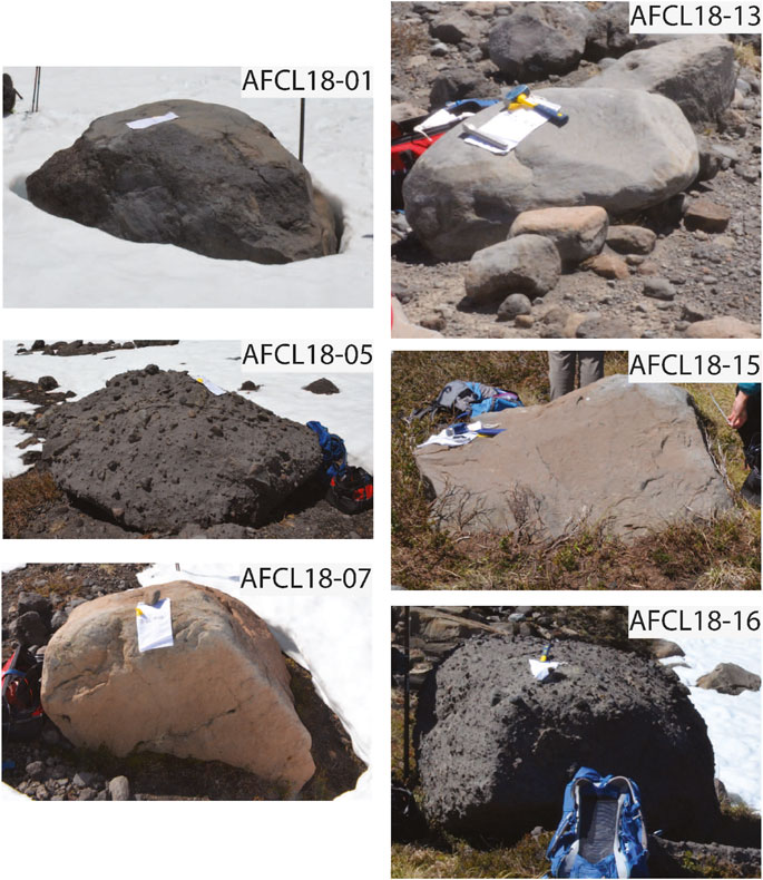
FIGURE 5. Representative basaltic boulders (conglomerates and fine-grained crystalline) sampled for 36Cl surface exposure dating.
Whole rock samples were sawed to a measured thickness of between 0.4 and 2.0 cm before crushing and sieving to collect grains between 250 and 125 µm. Chemical preparation of samples was conducted at the University of New Hampshire Cosmogenic Isotope Lab using a modified version of the protocols presented in Stone et al. (1996) and Licciardi et al. (2008). A key component of the modified procedures includes measuring 35Cl/37Cl on a ∼1 g aliquot of rock prior to 36Cl extraction and measurement on the full sample. The ∼1 g aliquot was spiked with a 37Cl-enriched solution (“LLNL Spike A”; 35Cl/37Cl = 0.93) and ∼4,000 µg of Br, which served to increase the size of the final precipitate. Total sample Cl was determined through isotope dilution methods. 36Cl was extracted as Ag(Cl,Br) from full rock samples in two analytical batches following standard procedures. All samples received a carrier solution containing ∼4,000 μg of Br and a natural ratio Cl carrier (35Cl/37Cl = 3.127). This technique was used to better control the total Cl within the analytical batch and reduce potential AMS memory effects (Arnold et al., 2010; Finkel et al., 2013).
Measurements of 35Cl/37Cl and 36Cl/37Cl were conducted using the 10 MV tandem accelerator at the Lawrence Livermore National Laboratory Center for Accelerator Mass Spectrometry (LLNL-CAMS). Analytical uncertainty on 35Cl/37Cl measurements ranged from 0.42 to 0.45%. Analytical uncertainty on 36Cl/37Cl AMS measurements was between 4.3 and 13%. Sample 36Cl concentrations are corrected for lab background using an average blank value for the two analytical batches (4.12 × 10⁴ atoms 36Cl, n=2). Major and trace element concentrations in the samples were determined using x-ray fluorescence and inductively coupled plasma mass spectrometry at SGS Mineral Services in Burnaby, British Columbia, Canada. Analytical data used to determine surface exposure ages are provided in Table 3.
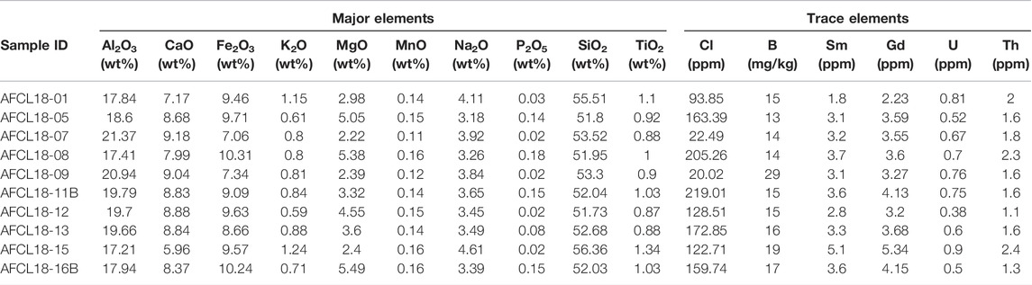
TABLE 3. Elemental composition measured on whole rock samples after leaching. Major elements are in wt%, and trace elements in ppm unless noted otherwise.
Moraine boulder exposure ages were calculated using a developmental version of the CRONUS-Earth 36Cl calculator (Balco et al., 2008; http://stoneage.ice-d.org/math/Cl36/v3/v3_Cl36_age_in.html) and LSDn scaling (Table 2; Lifton et al., 2014). The 36Cl calibration datasets applied by the calculator can be found in the ICE-D database at http://calibration.ice-d.org/allcds. Based on field observations, no corrections were made for rock surface erosion, vegetation cover, or snow coverage. A bulk density value of 2.7 was used for all samples. All cosmogenic ages here are presented as years prior to sampling (AD 2018).
We made corrections for nucleogenic 36Cl production using a rock formation age of 130 ka (Muñoz et al., 2011). Nucleogenic 36Cl is produced in moderate amounts when 35Cl absorbs neutrons released by the decay of U and Th isotopes (Gosse and Phillips, 2001). In rocks with high Cl, U, or Th concentrations, nucleogenic 36Cl can thus constitute a substantial proportion of the total 36Cl. In typical exposure age calculations, the amount of nucleogenic 36Cl in a sample is calculated assuming steady state production, and that value is subtracted from the total 36Cl to obtain the cosmogenic component (Marrero et al., 2016b). However, in young rocks (<1 Ma formation age), production and decay of nucleogenic 36Cl may not be in equilibrium, and erroneously assuming steady state could lead to uncertain and/or inaccurate surface exposure age determinations (e.g., Sarikaya et al., 2019; Anjar et al., 2021). To assess the sensitivity of our 36Cl ages to the time of rock formation, we also calculated 36Cl ages assuming a rock formation age of 30 ka. Calculated surface exposure ages presented in the results and discussion of this study use a rock formation age of 130 ka to represent the last stage of volcanism on Monte Sierra Nevada based on lack of visual evidence of younger vents or deposits to support a formation age of 30 ka (Muñoz et al., 2011). Surface exposure ages representative of a younger date of rock formation of 30 ka are presented in Supplementary Table S1, as a possible late Pleistocene formation age has not been dismissed by available evidence.
Dendrochronology was used to obtain an approximate date of establishment for Araucaria araucana (Pewén) trees growing on the most distal moraine in the valley, to provide an independent minimum age of moraine formation and deglacial processes. To assess the minimum age of the moraine, increment borers were used to collect samples from mature A. araucana trees atop the outermost moraine (M1) of the proglacial area of the study site (Figure 3). These trees were selected with consideration to morphological attributes such as bark, height, diameter, as well as size and form of branches, all visual characteristics associated with old A. araucana trees. Two cores per tree from A. araucana (n=35) were extracted from living trees growing on the site using the aforementioned criteria, forming the “NEV” chronology. Samples were taken at 1.3 m from the soil, to assess a minimum age of the trees. Tree cores were then sanded for visual identification of growth rings (Stokes and Smiley, 1996), in order to be counted and measured in the Laboratory of Dendrochonology and Environmental Studies at Pontificia Universidad Católica de Valparaíso, Chile (https://www.pucv.cl/uuaa/site/edic/base/port/dendrolab.html). Ring width was measured to ±1 µm resolution using a Velmex system (https://www.velmex.com/), after which the COFECHA software (Holmes, 1983) was used to assess and corroborate the dating of each tree using the ring width measurement patterns across the suite of tree cores. Of the 35 sampled trees, 30 were able to be properly cross-dated. From these 30 trees, 20 exhibited curvatures close to the pith. We selected the five oldest trees that exhibited this curvature, suggesting a minimal age close to the total age of the tree, and using the Duncan method (Duncan, 1989) estimated the number of missing rings. The age of the oldest tree was used to provide an independent and cross-dated minimum age of the glacial landform from which the trees had colonized.
We applied a modified version of DETIM by Hock (1999), which is available at http://regine.github.io/meltmodel/. As inputs, we used a climate file from the Global Historical Climatology Network (GHCN) (https://www.ncei.noaa.gov/products/land-based-station/global-historical-climatology-network-daily) with daily data from AD 2004–2013 (Temuco station, Figure 1), as well as the gridded NASADEM surface. The model also requires gridded surfaces for aspect and slope values that were calculated using the spatial analyst tools in ArcGIS 10.4.1. The model ran on the Cygwin64 C compiler following the approach of Stansell et al. (2022). The model ran with degree-day factors (DDFs) for ice and snow of 7 and 3.5 mmw. e. K−1 d−1, values typically used for Chilean glaciers (Möller and Schneider, 2010).
The climate input file requires some pre-processing of climate data, including the calculation of a precipitation gradient and temperature lapse rate. The precipitation amount was set at a value of ×1.5 the values recorded from the Temuco station, which is similar to what is observed at other GHCN stations of similar elevation offsets in the region. No lapse rate was applied to the precipitation amounts along the glacier profile.
The model also requires an estimated temperature offset (Tdiff) corresponding to the location of the oldest mapped moraine (M1), which we independently determined by finding the difference between present (pr) and past (pa) Equilibrium Line Altitudes (ELAs) and applying a simple linear relationship using a lapse rate of 6.5°C/100 m:
We used the Area Altitude Balance-Ratio (AABR) method (Osmaston, 2005) to determine ELAs. The AABR method estimates the ELA using the hypsometry of the glacier or the proglacial area within the limits of former ice extents, usually demarked by moraines. We used the 12.5 pixel size DEM available from ALOS PALSAR imagery as a source of topographical information to build the hypsometric curve (ASF DAAC, 2015), and a 3-m resolution true-color composite from the Planet Constellation to interpret the glacier margin in 2013 and to derive ELApr. For the past hypsometry, we trimmed the ALOS DEM extending the current margin by following the pattern of the trimline to the moraine crest closest to the cliff (M1). For the calculation, the method iteratively searches the elevation of the zero-balance, assuming that the mass balance gradient is linear, with a steeper slope in the ablation zone (Kaser and Osmaston, 2002). A key component of this approach is to select a suitable ratio between mass balance gradients, which can be computed from mass balance observations and assumed to hold in the past. In our case we face the challenge that almost no mass balance data exists for the region. The few direct measurements available from the Mocho Glacier (Rivera et al., 2005; Schaefer et al., 2017), situated about 115 km to the south, suggest a balance ratio of 3.2, larger than figures commonly used, such as 1.75 or 2 (Osmaston, 2005). A recent study found that a value of 1.56 represents glaciers at a global scale, although with important spread (Oien et al., 2021). Guided by these studies, we tested several ratios, opting for 2.38 as a best approximation to represent this region. We notice, however, that the difference in ELAs between ratios of 1.56 and 3.2 is 47 and 77 m for the present and the past, respectively, which translates to an uncertainty of 0.2°C. Using the median AABR value of 2.38 results in an ELApr and an ELApa of ∼2,267 m a.s.l. and ∼2029 m a.s.l. This change in ELA (ΔELA) of -238 m translates to Tdiff of ∼−1.5°C.
We then ran the DETIM with multiple climate scenarios. First, the model was run over the interval from A.D. 2004 to 2013 with no change in temperature and precipitation relative to today. Next, we ran the model with 1.5°C cooling and a 20% increase in precipitation as a first approximation to simulate Neoglacial conditions that are represented by the AABR method. We assumed wetter conditions were associated with ice advances because proxy and modeling studies suggest that this region had increased precipitation amounts at times when it was colder during the Late Holocene (Bertrand et al., 2014). In order to test glacier sensitivity, we also ran the model with temperature changes of +1°C with a doubling of precipitation amounts. A series of other tests were run by changing only one variable at a time using ±1°C change in temperature, ±20% change in precipitation, and lapse rates ranging from 0.55°C/100 to 0.75°C/100. Additionally, to test the influence of DDFs, we adjusted the ice and snow values by ±1, following the approach of Möller et al. (2007).
Finally, we applied the flow model of Plummer and Phillips (2003) to simulate glacial thickness using the input of the mass balance grid. While the mass balance model identifies areas of ablation and accumulation, the flow model predicts the shape, size, and extent that a glacier stabilizes at for those conditions at steady-state. The model applies the standard flow law for ice using the shallow ice approximation, and using multiple interpolation methods. The results of the combined energy mass balance and flow models are shown in Figure 6. For all model runs, we present the lowest altitude of ice limit, maximum and average ice thickness values (Table 4).
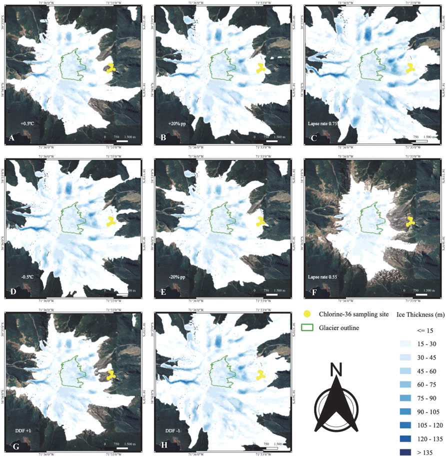
FIGURE 6. Google Earth image of Monte Sierra Nevada with ice thickness results from the combined mass balance and flow models superimposed. The yellow circles mark the locations of dated moraine positions from this study, the modern glacial outline is represented in green. From top left to bottom middle. (A) Temperature increase of 0.5°C. (B) Precipitation increase of 20%. (C) Lapse rate of 0.75°C/100 m. (D) Temperature decrease of 0.5°C. (E) Precipitation decrease of 20%. (F) Lapse rate of 0.55°C/100 m. (G) DDF of +1. (H) DDF of -1.
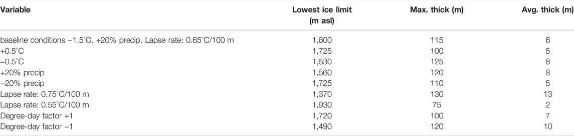
TABLE 4. Parameters used for modeling of the glacial mass energy balance sensitivity analysis.
The surface exposure ages of moraines on Monte Sierra Nevada range from 4.2 ± 0.2 ka to 0.28 ± 0.05 ka, and represent multiple phases of glacial growth and decay (Figure 7; Table 2). Sample AFCL18-16B, located on the most distal moraine in the valley, M1, is dated to 4.2 ± 0.2 ka. A second boulder sampled from M1, AFCL18-15, yielded a younger age of 0.65 ± 0.12 ka. Two samples dating to 2.1 ± 0.1 and 0.79 ± 0.08 ka are located on moraine M2, near the cliff on the north end of the valley. On the center moraine of the complex, M3, samples dated to 0.39 ± 0.05 and 0.28 ± 0.05 ka. Three samples from M4 yielded exposure ages of 2.6 ± 0.1, 0.46 ± 0.07, and 0.42 ± 0.06 ka. On M5, the innermost moraine in the valley, a single sample dated to 0.82 ± 0.09 ka. No apparent age biases (e.g., too young or too old) were detected between the fine-grained crystalline vs the basaltic conglomerate source rocks.
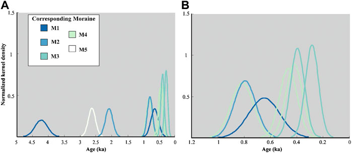
FIGURE 7. Panel (A) Normalized kernel density estimates for all samples. Panel (B) Normalized kernel density estimates for samples that fall within the Southern Hemisphere expression of the Little Ice Age. Sample ages in both panels are plotted with internal analytical uncertainties.
The cross-dating process resulted in an inter-correlation value of 0.55, a high correlation for A. araucana ring width chronologies (Muñoz et al., 2014). The five oldest trees comprising the NEV chronology, which showed a complete curvature close to the pith, were established between five and six hundred years ago. The first rings in samples from this group of trees were developed around the years AD 1407, 1462, 1511, 1559, and 1609. With the addition of missing rings due to the exhibited curvature (Duncan, 1989), the first ring for each of these five trees results in an approximate year of AD 1318, 1378, 1482, 1535, and 1580, respectively. The oldest tree of the NEV chronology yielded a date of AD 1318, providing a minimum limiting age of moraine M1 at 0.70 ka. This tree cross-dated to 0.54 with the complete set of trees measured, a value close to the mean inter-correlation value at this site, corroborating the age of this tree. Finally, due to the height of the extraction (1.3 m from the ground), a number of rings were missing with respect to the complete age of the trees, leading to an underestimation of the age of each tree. As such, a number of years, not determinate, should be added on to the determined age after ring counting, necessary to obtain the growth height observed. Following Lusk and Le Quesne (2000), the mean height growth rates of A. araucana were 169 mm/year in sun-grown trees, and 111 mm/year in shade-grown individuals. Considering these estimations, a minimum period of around 10 years should be added to the age of each tree. However, depending on competition and site requirements, this period could be longer than 10 years.
The combined glacier mass balance and flow models produced simulated ice extents that mimic the modern and paleo-conditions. Using the GHCN temperature and precipitation values produced an ice margin at an elevation (∼1905 m) that is similar to today. Using a cooling of 1.5°C and a 20% increase in precipitation produced a modeled ice extent that is similar to the outer-most mapped and dated moraines on Monte Sierra Nevada (Figure 6). As the moraine complex represents an elevation change of only ∼19 m over a distance of ∼350 m, distinguishing between moraines on the gridded volume proves difficult. In general, the model produces the thinnest ice near moraine positions and thicker ice elsewhere. Glacial coverage on Monte Sierra Nevada also tends to be thicker on the eastern slopes that are less steep than the western slopes. For modeling purposes, we assumed that periods of colder temperatures were associated with wetter conditions over the last several millennia (see Discussion). Nevertheless, the sensitivity analysis indicates that varying temperature alone by ±0.5°C shifted the elevation of the lowest ice position by ∼±130 m, while adjusting precipitation by ±20% shifted the ice margin by ∼−40 and +125 m (Table 4). Shifting the lapse rate by ±1.0°C/100 m offset the lowest ice position by −230 and +330 m. Lastly, shifting the DDF values by ±1 offset the lowest ice limit by +120 and −110 m.
The exposure ages presented here are some of the youngest to be developed using 36Cl methods on glacial boulders in the Andes. While our dataset includes only a modest number of ages, these results demonstrate the feasibility of using 36Cl to date young glacial deposits of similar compositions elsewhere in the Chilean Andes. Due in part to the small number of boulders, definitive and discreet ages cannot be confidently assigned to each moraine position. However, the chronology established for this moraine complex provides clear documentation for multiple phases of retreat and readvance of Monte Sierra Nevada glacier during the Late Holocene.
Multiple sources of uncertainty must be considered when using 36Cl to date Late Holocene moraine boulders. Processes such as post depositional erosion and boulder rotation can contribute to uncertainties in surface exposure dating (e.g., Balco, 2020). In addition, the presence of nucleogenic (i.e., non-cosmogenic) 36Cl in rock surfaces can introduce considerable uncertainty to exposure age calculations. In a setting such as Monte Sierra Nevada, where the target landforms for dating and the lithologic units are likely relatively young, low-energy neutron capture can also produce non-negligible amounts of 36Cl. In exposure age calculations, the nucleogenic 36Cl must be subtracted from the total 36Cl to obtain the concentration of cosmogenic 36Cl. At this time, 36Cl production rates from low-energy neutron capture are the least well-characterized production pathway (Marrero et al., 2016a), partially because low-energy neutron flux depends on difficult-to-constrain paleoenvironmental factors such as snow cover and presence of water (Zreda et al., 1993; Phillips et al., 2001; Schimmelpfennig et al., 2009; Zweck et al., 2013; Dunai and Lifton., 2014). Improved constraints on the timing of volcanic episodes of Monte Sierra Nevada will help to fully evaluate the nucleogenic production of 36Cl in the Monte Sierra Nevada moraines, as these Pleistocene deposits have likely not reached steady-state production for nucleogenic 36Cl (Sarikaya et al., 2019; Anjar et al., 2021). With these considerations in mind, we applied recent advances in 36Cl methods to produce robust ages for the last several millennia.
The cosmogenic 36Cl ages from Monte Sierra Nevada suggest glaciers in the CSCh Andes fluctuated throughout the latest Middle and Late Holocene. Ice margin retreat from the oldest and most distal moraine, M1, likely commenced by ∼4.2 ± 0.2 ka based on sample AFCL18-16B (Figure 3). A second boulder sampled from M1 to the north of the stream yielded a much younger age (AFCL18-15; 0.65 ± 0.12 ka), which aligns with the establishment of A. araucana trees on this glacial landform by 0.70 ka. Additional exposure samples are needed from moraine M1 to further assess the potential of nuclide inheritance due to unknown timing of boulder stabilization over melting debris covered ice, as well as to produce a statistically robust age determination of this landform. However, the morphology of the M1 moraine might aid in deciphering this complex glacial setting. The subtle duel-crested nature of the southern extent of M1 and observed pedogenesis on the moraine surface (Jenny, 1944; Mason and Jacobs, 2018) may suggest that M1 demarcates an expansion of the ice front prior to 4.2 ± 0.2 ka, and again before 0.65 ± 0.12 ka. Prior to 0.65 ± 0.12 ka the glacier likely expanded to the position of moraine M1, resulting in reoccupation of this landform, abutted the ice-proximal expression of M1 formed in the mid-Holocene, and shaped the dual-crest observed on the southernmost extent. The glacier then commenced its final retreat from the M1 position by ∼0.65 ± 0.12 ka.
The composite nature of moraine M1, with a potential formation in the mid-Holocene followed by a latest Holocene glacial advance reoccupying this landform, would allow for a period of several thousands of years for soil development to occur. While soil may develop rapidly on deglaciated terrain, this process is largely dependent on environmental factors such as humidity and precipitation, as well as weathering rates of the original parent material (Mason and Jacobs, 2018). The lack of soil development on moraines M2-M5, along with an initial colonization age of moraine M1 by A. araucana trees of 0.70 ka, suggests that attributing a younger moraine formation age of ∼0.65 ± 0.12 ka would preclude sufficient time for pedogenesis to support the colonization of A. araucana on that landform. When combined, these independent datasets suggest glaciers were at more advanced positions in the region just prior to ∼4.2 ka, and supports assigning M1 an initial mid-Holocene formation age.
The trimline abutting M1 along the southern ridge of the valley suggests these features formed concurrently, and while no samples were dated from up-valley of the moraine complex, we suggest the trimline formed contemporaneously with M1. The continuation of the trimline along the southern ridge up-valley of the chute suggests that ice from the cirque directly up-valley from the dated moraines contributed to the formation of M1 in the mid-Holocene. However, this up-valley source of ice was likely minimal during the Late Holocene, with ice predominantly flowing over the southern ridge from the adjacent valley, as interpreted from the cross-cutting stratigraphy of the chute eroding a portion of the trimline (dashed blue, and black lines respectively, Figure 3). The modeling results suggest that greatest ice thicknesses in the valley were obtained when the ice margin expanded past the mapped extent of the moraine complex, which based on both the exposure ages and dendrochronology, has not occurred in the Late Holocene. Thus, this expression of high ice thickness in the valley likely formed during a period of glacial expansion during the mid-Holocene, predating glacial retreat from the M1 position at ∼4.2 ± 0.2 ka. The glacier then retreated to an up-valley position before retreat halted. During this interval of glacial recession, ice from the cirque likely retreated up valley, separating from the glacial tongue flowing over the saddle on the southern ridge.
Four samples (AFCL18-01; 2.6 ± 0.1 ka, AFCL18-05: 0.81 ± 0.09 ka, AFCL18-12; 2.1 ± 0.1 ka, and AFCL18-13; 0.79 ± 0.08 ka) date from 2.6 ± 0.1 ka to 0.79 ± 0.08 ka, and are located at the northern and southernmost extents of the moraine complex (Figure 3). The exposure ages obtained from these samples support a fluctuating ice margin, and initial exposure from the subglacial environment predating a final glacial advance in the valley during the latest Holocene. The mapped locations of these samples at the outermost extents of the moraines on which they are perched suggests reworking and transport to their present locations by one or more readvances of the glacier. Additionally, the older exposure ages of these marginal samples compared to samples closer to the center of the moraine complex supports the likelihood of multiple stages of ice marginal expansion. Ice flow directions assessed from striated surfaces (Figure 3) indicate a radial advance of glacial ice in the valley, which would have obliterated previously formed moraines, and redeposited these boulders in more lateral positions of the moraine complex. These samples may have originally been deposited on the valley floor during recession of the ice margin, or were potentially exposed from subglacial conditions on the southern ridge. Additionally, these samples may have variable amounts of 36Cl inheritance, which could explain some of the scatter seen in the available ages. Finally, these boulders may have experienced destabilization and subsequent rotation as underlying ice melted, an inherent pitfall to interpreting surface exposure ages on ice-cored moraines.
The youngest surface exposure ages (AFCL18-07, 0.42 ± 0.12 ka; AFCL18-08, 0.46 ± 0.07 ka; AFCL18-09, 0.40 ± 0.05 ka; AFCL18-11B, 0.28 ± 0.05 ka; and AFCL18-15, 0.65 ± 0.12 ka), and the development of moraines M2-M5 provide evidence for multiple phases of ice expansion in the valley over the latest Holocene. Two scenarios are plausible to explain the formation of moraines M2-M5 between this final glacial advance and the modern. The first would entail a glacier with minimal to no debris coverage commencing a continuous pulsed retreat of the ice marginal environment from 0.65 ± 0.12 ka through the modern, emplacing moraines M2-M5. However, it is more likely that during this interval, and perhaps the entirety of the Holocene, that the lower portion of the glacier was debris-mantled, as debris coverage on many regional glaciers has been increasing in modern times (Glasser et al., 2016). If the glacial snout was indeed debris-mantled, the response of the ice marginal environment to climate-driven changes could be more muted (Kirkbride and Warren, 1999; Naito et al., 2000; Davies and Glasser, 2012).
Critically thin ice margins along the frontal edge of the glacier likely resulted in instability of slope angles on moraine M1, and potentially along the northern and southernmost lateral positions of the other moraines in the complex, leading to partial or full collapse and deposition of supraglacial debris. Several exposure ages towards the center of moraines M3 (0.40 ± 0.05 ka) and M4 (0.42 ± 0.12 ka and 0.46 ± 0.07 ka) are in close agreement. The location of these samples may have been better insulated from more rapid fluctuations of the ice margins at the time collapse was initiated, as surface melt rates often vary spatially depending on the thickness of debris coverage (Östrem, 1959; Moore, 2018). The timing between the final abandonment of moraine M1 at 0.65 ± 0.12 ka and the exposure of boulders on the central portions of moraines M3 and M4 at ∼0.4 ka may represent an interval when climatic conditions were cooler and wetter, resulting in temporary stabilization of the ice margin at moraine M3. Furthermore, the cluster of ages on moraines M3 and M4 between 0.46 ± 0.07 ka and 0.40 ± 0.05 ka might suggest that latest Holocene warming and/or drying resulted in ice surface lowering, the melt out of supra- and englacial debris, and the continued recession of the ice margin up valley. However, as debris can either increase insulation or enhance ablation of the glacial ice depending on both the thickness and extent of coverage (Davies and Glasser, 2012; Bartlett et al., 2021), further data and modeling are needed to substantiate these tentative interpretations.
On the ice-proximal side of moraine M5 to the north of the stream, hummocks were surveyed (Figure 3, Figure 4). The area over which hummocks are observed has been substantially dissected by an immature drainage network that has also eroded large sections of moraines M4 and M5. Development of this chaotic terrain suggests a rapid retreat from the location of moraine M5 (Owen and England, 1998; Figure 3). The development of hummocks also supports the idea of a debris-covered glacier in the lower reaches of the valley, particularly along the glacial snout (Anderson, 2000; Bartlett et al., 2021). An abundance of observed glacial scree and talus deposits in the valley, particularly along the southern ridge of the valley, would provide sufficient source material to generate debris coverage of the snout of the paleo-glacier (Shakesby et al., 1987; Giardino and Vitek, 1988; Moran et al., 2016; Charton et al., 2021b). As the talus is most extensive beneath the trimline and covering the chute along the southern ridge of the valley, debris coverage of the lowest extents of the glacier most likely increased following the initial abatement from the M1 location and thinning of the glacial surface.
Moraines M4 and M5 to the north of the stream are also weakly preserved, potentially indicating that these moraines were ice-cored, where dead ice would possibly be entrained along with glacial debris (Evans, 2009). Deflation of these glacial landforms would occur as the ice core melted, resulting in the poor preservation observed, and the destabilization of perched boulders (Putkonen and Swanson, 2003; Briner et al., 2005). A debris-mantled glacier would present a possible explanation in the scatter of the cosmogenic ages from this study site, such as the younger exposure age of sample AFCL18-11B (0.28 ± 0.05 ka) on M3, as it may have experienced some rotation due to debris coverage limiting ablation and the enhanced likelihood of boulder rotation upon destabilization.
The glacier modeling results and geomorphic evidence provides additional support that the present-day ice cap system was more extensive at times during the Late Holocene. Our model indicates that as the ice cap expanded, it likely covered more ridges and had additional source-ice regions with more complex ice-flow dynamics down-valley than what is seen in present-day (Figure 6). These complex ice patterns likely explain part of the scatter of available ages as the glacier did not follow a standard down-valley glacier pathway in the latest Holocene. Additionally, an eroded trimline indicates ice was flowing from south-to-north in the valley from a ridge that is currently ice-free (Figure 3). Combined, this evidence supports the initial formation of moraine M1 via a combination of glacial ice flow from the cirque of the modern glacier, merged with ice sourced from the valley directly to the south via the saddle along the southern ridge, and possibly the north side of the valley as well (Figure 3). The eroded trimline feature also suggests that following the abandonment of the M1 position at ∼4.2 ± 0.2 ka, glacial ice was likely sourced solely from the southern ridge of the valley with little to no contribution directly down-valley from the glacial cirque. That ice then flowed outward in a radial piedmont-style pattern across the table-top-like valley floor to reoccupy M1, and to the positions of moraines M2-M5 as supported by the striated surfaces throughout the lower extents of the valley.
Our chronology of Late Holocene glacial fluctuations from Monte Sierra Nevada is further augmented with independent tree-ring data collected near the margins of the apparent trim-line (Figure 3). The 36Cl ages suggest that a Late Holocene retreat of the frontal/lateral margin occurred at ∼0.65 ± 0.12 ka. While the chronology of the oldest tree provided by the NEV record only extends to 0.70 ka, it provides a minimum-limiting age of glacial retreat from M1. It is possible that this landform has been colonialized by successive generations of A. araucana trees, as very few specimens have been dated to older than 500 years (Aguilera-Betti et al., 2017). Additionally, the period necessary between moraine stabilization and seedling establishment depends in part on the soil evolution of the landform to provide conditions for germination and growth, as well as individual species capacities to grow under limited conditions. This period could take several decades in most cases. However, A. araucana is a recognized species that can grow on low developed soils (Veblen, 1982). This, combined with the time required for the tree to grow to the height at which cores were extracted, results in a likely formation age of moraine M1 at minimum a few decades prior to 0.70 ka, further suggesting the true age of the moraine is older than 0.70 ka.
The modeling results presented here provide a physical and quantitative basis for interpreting glacial variability at Monte Sierra Nevada, and despite not being fully capable of handling the complex dynamics of a debris-mantled glacier, the Temperature-Index approach provides an important first-order estimate at quantifying paleo-environmental conditions on Monte Sierra Nevada. Additionally, the interpretation of a debris-covered glacier for this valley concerns only the snout, not the entire ablation area, and even less of the whole glacier surface. On modern decadal timescales, the dynamics of debris-covered glaciers are observed to operate differently than clean glaciers, but very little research exists to determine whether debris cover exerts a significant effect on the temperature sensitivity at centennial to millennia scales. Furthermore, when climate trends are strong, debris-cover does not cause a significant insulation effect (Burger et al., 2019), suggesting that under certain scenarios, in particular considering relatively persistent climate changes, debris-coverage does not alter glacier sensitivity significantly.
This model was parameterized with a range of representative temperature and precipitation values from the AABR calculations, suggesting temperatures were ∼1.5°C colder and precipitation was ∼20% higher during peak Neoglacial ice advances over the last several millennia. It is presently unclear, based on the available chronology, whether the peak Neoglacial ice advance at Monte Sierra Nevada was associated with the LIA or an earlier advance. However, the modeling outcome is generally the same regardless of the chronology when recognizing that it was wetter when it was colder at multiple times during the Neoglacial (Bertrand et al., 2014). Following this assumption, we were able to achieve ice margin reconstructions that match the mapped moraine positions on the landscape (Figure 6). The sensitivity analysis also highlights that a 20% increase in precipitation offsets a temperature shift by ∼0.5°C, which is less than other modeling studies that suggest a doubling of precipitation is needed to offset a ∼1°C temperature change (Figure 6; Sagredo et al., 2014). The results also highlight that multiple combinations of climate parameters are capable of explaining glacial variability in this region, and these modeling scenarios will improve as independent proxy evidence of Late Holocene environmental conditions, such as tree-ring records, continue to be developed.
The results presented here are not of sufficient resolution to attribute confident alignment of this record of glacial fluctuations to either the “Aniya-type” or “Mercer-type” chronology of Neoglacial events (Figure 8), however, certain similarities exist. Event I of Aniya (2013) is proposed to have occurred at ∼5.0 to 4.3 ka, while Mercer (1976) designates a first Neoglacial advance between 4.6 and 4.1 ka. Thus, the timing from both chronologies is similar to the oldest, outermost moraine age of 4.2 ± 0.2 ka. No samples dated in this study fall within the event II range of the “Aniya-type” chronology (3.7–3.4 ka), suggesting that either the climatic conditions in CSCh did not support a glacial advance during this interval, or that evidence of this event locally was destroyed by subsequent Neoglacial ice fluctuations. As the two exposure ages from this study (2.6 ± 0.2 ka and 2.1 ± 0.1 ka) that overlap with Mercer’s second event and Aniya’s III event are from proposed reworked boulders, we cannot assess any overlap in glacial advances from these samples. Similarly, while two exposure ages developed from our study (0.81 ± 0.09 ka and 0.79 ± 0.08 ka) fit into the event IV range (1.4–0.7 ka) of the Aniya chronology, we are unsure if these samples were recycled from a previous exposure due in part to sample placements at the far northern and southern lateral extents of the moraine complex. The latest Holocene glacial readvance is assigned an approximate range of 0.57 to 0.27 ka in the Mercer (1976) chronology and 0.52 to 0.3 ka (event IV) in the Aniya (2013) chronology. Four of the developed exposure ages from this study fit into this interval (0.46 ± 0.07 ka, 0.42 ± 0.12 ka, 0.40 ± 0.05 ka, and 0.28 ± 0.05 ka) of the Southern Hemisphere expression of the LIA. However as previously discussed, these ages are distributed across two moraines, M3 and M4 (Figure 3), precluding a definitive assessment as to which moraine represents the LIA with the current data set.
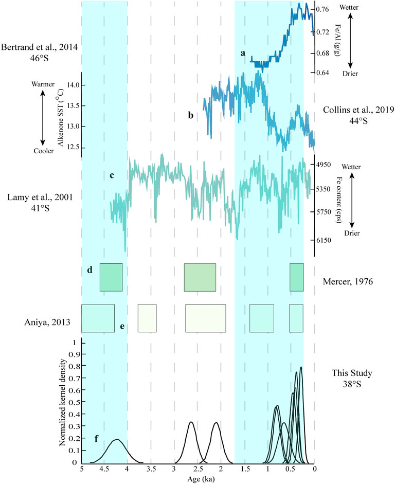
FIGURE 8. From top to bottom: (A) Ratio of Iron (Fe) to Aluminum (Al) (g/g) from sediment core PC29A retrieved from Quitralco fjord (46°S), as a proxy for precipitation seasonality. An increase in Fe/Al is interpreted as increased precipitation regionally due to latitudinal variations in the position of the SWWB (Bertrand et al., 2014). (B) An alkenone based proxy record for SST (°C) from oceanic sediment core MD07-3093 (44°S) (Collins et al., 2019). (C) Iron (Fe) intensity (cps) from oceanic sediment core GeoB 3313-1 (41°S), as a proxy for position of the SWWB. Decreased Fe intensity is interpreted as the SWWB located in a more northerly position compared to the study location, resulting in wetter conditions regionally (Lamy et al., 2001). (D) Timing of “Mercer-type” glaciations in Southern Chile (Mercer, 1976). (E) Timing of “Aniya-type” glaciations in Southern Chile (Aniya, 2013). (F) Chlorine-36 surface exposure ages from this study. Blue vertical bars indicate assessed intervals of SAM negative phases (cold and wet), inferred from the Lago Cipreses sediment core record (51°S) (Moreno et al., 2018).
Slightly different regions were assessed to build the afore mentioned chronologies. The Mercer-type chronology evaluated a latitudinally longer corridor of glacial records from 39°S to 53°S, while the Aniya-type chronology was slightly more restricted and was compiled from records sourced from between ∼46°S and 52°S. Additionally, the inclusion of records from tide-water glaciers as opposed to a restriction of the analysis to fully terrestrial based glacial systems could potentially result in more variability in age control in these records. As highlighted by Glasser et al. (2004), the differences between the Aniya-type and Mercer-type chronologies are also likely more related to dating uncertainties and the lack of bracketing age control rather than actual differences in interhemispheric glacier behavior. The “Aniya-type” chronology though widely recognized, was developed largely from 14C dating of organic material combined with tree-ring data and lichenometry (Aniya, 1995; Aniya, 1996). Since the establishment of these chronologies numerous advancements have been made in various dating methods (i.e., cosmogenic nuclide exposure age dating, optically stimulated luminescence, tephrochronology, etc.) providing researchers a lens through which age constraints on regional records can be reexamined. Nevertheless, additional multi-proxy approaches similar to what we present here for Monte Sierra Nevada are needed as researchers work to develop comprehensive chronologies of past glacial variability in the high-latitude Andes.
The data reanalysis on the Patagonian Ice Sheet published by Davies et al. (2020) includes recalibrated chronologies of glacial fluctuations, but notes that the Late Holocene is not yet well understood over large regions of southernmost South America. However, three intervals of Neoglacial advances were well supported from the studies reviewed within: in the mid-Holocene at 5 ka, a smaller Late Holocene advance between 2.0–1.0 ka, and a LIA advance between 0.5–0.2 ka (Davies et al., 2020). Our proposed advance prior to 4.2 ± 0.2 ka, and the cluster of ages that fall within the LIA (0.46 ± 0.07 ka, 0.42 ± 0.12 ka, 0.40 ± 0.05 ka, and 0.28 ± 0.05 ka), are supported by this large-scale assessment from the Patagonia Ice Sheet. Nevertheless, our ability to disentangle how much past glacial variability in the Chilean Andes was driven by climate-related processes versus hypsometric controls will improve as we continue to apply more comprehensive dating methods, including additional direct ages on moraine boulders.
Andean glaciers have varying sensitivities to temperature and hydrologic changes depending on location, geometry and other local and regional factors (e.g., Sagredo et al., 2014). CSCh glaciers are typical of mid-latitude glaciers, with mass balance sensitivities that are seasonal and seemingly most sensitive to summer temperatures and winter precipitation (Masiokas et al., 2008). These temperature and precipitation anomalies are tightly coupled, with cold intervals corresponding to wetter periods and vice versa (Masiokas et al., 2009). Modern ice fields and outlet glaciers in Chile have historical mass balances that are sensitive to both atmospheric temperature and precipitation changes (Bown and Rivera, 2007; Casassa et al., 2007). Since 1975, the regional freezing level (0°C isotherm) has risen by ∼120 m in winter and 200 m in summer (Carrasco et al., 2005), with an overall increase of 0.25°C/decade in mean annual temperature since 1979 (Falvey and Garreaud, 2007). There has also been a strong negative trend in winter precipitation amounts over the last century (Masiokas et al., 2008).
Even though the annual cycles of temperature and precipitation vary across the Andes, it is possible that Pacific oceanic-atmospheric forcing synchronized climate variability across the low and high southern latitudes during much of the Late Holocene. For example, it has been proposed that SAM and ENSO are teleconnected and possibly related on centennial time-scales, providing one possible explanation for Southern Andean glacial variability (Moreno et al., 2018). It is also possible that changes in the position of the SWWB drove much of the observed pattern of Neoglaciation as these winds deliver critical precipitation to Patagonian glaciers (Glasser et al., 2004; Kaplan et al., 2016). Millennial-scale SAM variability began after ∼5.8 ka (Moreno et al., 2018), and it is suggested that insolation combined with SAM drives millennial and centennial-scale glacier variability in southern South America through the Holocene (Reynhout et al., 2019). An increase in Southern Hemisphere summer insolation (assessed at 37°S) from the start of the Holocene through the modern (Berger and Loutre, 1991; van den Bos et al., 2018), would support the largest glacial expanse recorded in the valley, predating a retreat as early as ∼4.2 ± 0.2 ka. A warm and dry period during the Late Holocene (∼4.1–2.8 ka) has been associated with prolonged SAM-positive phases, resulting in less extensive glaciers (Reynhout et al., 2019), while after 2.8 ka conditions appear to reflect more SAM-negative conditions, becoming colder and wetter, similar to the proposed intervals of SAM phases by Moreno et al. (2018). These SAM negative phases roughly correspond to intervals of assessed glacial expansion on Monte Sierra Nevada (Figure 8). Additionally, ENSO variability might make SAM stronger due to the effect of atmospheric Rossby waves across the Pacific. These SST anomalies in the tropics drive pressure anomalies in the high latitudes, as positive phases of ENSO lead to negative SAM, and vice versa (Moreno et al., 2018).
There are multiple proxy records of wetter conditions and evidence of a northward shift of the SWWB from ∼0.82 to 0.22 ka (Figure 8; Lamy et al., 2001; Jenny et al., 2002; Bertrand et al., 2005; Fletcher and Moreno, 2012; Bertrand et al., 2014). Perren et al. (2020) suggests that the extratropical westerlies migrate northward during cold Neoglacial periods, and therefore, it seems likely that periods of increased precipitation were associated with colder temperatures. The tree-ring and glacier modeling results presented here further suggest that both increased precipitation and colder conditions drove the pattern of latest Holocene glacier variability.
Regardless of the degree to which temperature vs. hydroclimate were the dominant factors, Late Holocene glacial variability in the Chilean Andes was likely influenced by complex oceanic and atmospheric processes. For example, there appears to have been a close relationship between Pacific and Southern Ocean SSTs and atmospheric circulation during the Late Holocene. Oceanic SST records (44°S) demonstrate the connectivity between the Southern Ocean with increased ENSO variability, resulting in an ∼2.5°C cooling trend between ∼1.2–0.7 ka off the central Chilean coast (Figure 8; Collins et al., 2019). Additionally, precipitation proxy records suggest an equatorward or northward shift of the SWWB associated with colder SSTs and a southward shift associated with warmer SSTs (Figure 8; Bertrand et al., 2014). The SWWB delivers critical precipitation to temperate glaciers, especially on the windward side of the Andes (Bertrand et al., 2012) where a strong correlation exists between precipitation amounts and westerly wind anomalies (Garreaud, 2007; Moreno et al., 2009). Historical archives compared to meteorological data support this observation and suggest that some glaciers on the drier side of precipitation gradients in northern Patagonia have varied over the last several decades mostly in response to precipitation changes (Warren and Sugden, 1993). There is also a correlation between Pacific SSTs and freezing level height in the Andes (Bradley et al., 2009), suggesting that shifting ocean circulation and temperatures could drive both temperature and hydroclimate variability in CSCh.
Proxy and modeling results suggest that decreased radiative forcing due to reduced solar activity causes an equatorward shift in the mean position of the SWWB (Varma et al., 2011). During the LIA, reduced solar forcing combined with increased volcanic activity led to net global cooling (Mann et al., 2009; Miller et al., 2012). This cooling would likely have produced a similar equatorward shift in the SWWB and wetter conditions in CSCh Andes, driving the observed pattern of ice advances. The higher temperatures that followed the LIA likely led to a poleward shift in the SWWB, and drier conditions that combined, would have caused ice to retreat.
Our 36Cl-based chronology of latest-Holocene glacial fluctuations from the South-Central Chilean Andes includes some of the youngest developed surface exposure ages from this nuclide system in South America. Exposure ages and observed landforms in the valley suggest that the glacier was likely debris-mantled to some extent along the lower reaches of the valley, over the area of the mapped moraine complex. This scenario would suggest that moraine formation occurred only under periods of more enhanced climatic change regionally during the Late Holocene. In combining our moraine exposure age chronology with dendrochronology, and a geomorphic analysis of the valley we estimated the past glacial hypsometry in the valley, so as to numerically model the paleo glaciers response to regional climatic forcings. This model suggests that Monte Sierra Nevada glaciers most likely experienced phases of growth and decay under a range of temperature and precipitation conditions, predominantly exhibiting glacial expansion during periods of lower temperatures and increased precipitation over the last several millennia. These conditions were possibly driven by decreased SSTs associated with enhanced offshore upwelling, and increased regional humidity from a more northernly positioned SWWB. A more thorough understanding of South American climatic processes in the recent past, coupled with more precise chronologies, will shed light on regional climate trends and better identify the timing of apparently near global climate events such as the LIA. While we produced only a limited dataset for this study, we demonstrate the ability to date relatively young glacial landforms with multiple dating methods, which should help to improve our understanding of how complex mid-latitude oceanic-atmospheric dynamics are linked to low and high latitude climate changes, especially in the context of recent warming events. This study also highlights the need to better constrain the timing of Quaternary volcanic episodes in CSCh, which will improve the accuracy of 36Cl surface exposure dating in this young basalt-rich terrain and allow for a more precise characterization of regional glacial events. The record of glaciation produced here from Monte Sierra Nevada, along with additional records from other sites, will aid in assessing the sensitivity of glaciers in CSCh to Pacific Ocean-atmospheric processes throughout the Holocene, which is crucial as these glaciers are significant contributors to water availability regionally. Furthermore, in better constraining estimates of Andean alpine ice coverage throughout the Neoglacial period, global climate models will be better informed regarding complex cryosphere changes in albedo, continental temperatures of glaciated and recently deglaciated surfaces, and their associated drainage basins.
The original contributions presented in the study are included in the article/Supplementary Material, further inquiries can be directed to the corresponding author.
BP and NS led the writing of the manuscript with advisement from AF, JL, AL, and AM. AF, NS, AM, and EJC conceptualized the project, and wrote the National Geographic grant for initial funding. BP, AF, NS, EJC, and IC carried out the field investigation and sampling. BP, JL, and AL prepared and analyzed rock samples for 36Cl. NS, MS, AF, and TS modeled the glacial system. AM, EJC, and IG measured and calibrated the dendrochronology data. All authors have read, provided edits and agreed to the published version of this manuscript.
Funding for this work was provided by National Geographic (CP-119R-17), The Chilean Science Bureau (ANID) ANILLO ACT210080, The Center for Climate Action (PUCV ESR UCV 2095), The Center for Climate and Resilience Research (ANID, FONDAP N°15110009), and the Northern Illinois University Department of Geology and Environmental Geosciences Goldich Fund. Funding for publication of this manuscript was provided by the Northern Illinois University and University of New Hampshire Open Access Publication funds.
The authors declare that the research was conducted in the absence of any commercial or financial relationships that could be construed as a potential conflict of interest.
All claims expressed in this article are solely those of the authors and do not necessarily represent those of their affiliated organizations, or those of the publisher, the editors and the reviewers. Any product that may be evaluated in this article, or claim that may be made by its manufacturer, is not guaranteed or endorsed by the publisher.
The Araucanía region is part of the ancestral homeland of the Mapuche people. Monte Sierra Nevada is located on these occupied lands, and we recognize the Mapuche as the original and sustained stewards of this territory. We would like to recognize the provision of PlanetScope imagery under the research and education initiative, granted to AF and IC. We would also like to thank Bradley Singer for his expert assessment in estimating the age of volcanism at Monte Sierra Nevada. Additionally, we would like to thank both reviewers of our manuscript, who provided kind, constructive feedback, which led to the improvement of this publication.
The Supplementary Material for this article can be found online at: https://www.frontiersin.org/articles/10.3389/feart.2022.848652/full#supplementary-material
Aguilera-Betti, I., Muñoz, A. A., Stahle, D., Figueroa, G., Duarte, F., González-Reyes, Á., et al. (2017). The First Millennium-Age Araucaria Araucanain Patagonia. Tree-Ring Res. 73, 53–56. doi:10.3959/1536-1098-73.1.53
Alcalá-Reygosa, J., Palacios, D., Schimmelpfennig, I., Vázquez-Selem, L., García-Sancho, L., Franco-Ramos, O., et al. (2018). Dating Late Holocene Lava Flows in Pico de Orizaba (Mexico) by Means of In Situ-Produced Cosmogenic 36Cl, Lichenometry and Dendrochronology. Quat. Geochronol. 47, 93–106. doi:10.1016/j.quageo.2018.05.011
Álvarez, D., Fagel, N., Araneda, A., Jana-Pinninghoff, P., Keppens, E., and Urrutia, R. (2015). Late Holocene Climate Variability on the Eastern Flank of the Patagonian Andes (Chile): A δ18O Record from Mollusks in Lago Cisnes (47°S). Holocene 25, 1220–1230. doi:10.1177/0959683615580859
Ancapichún, S., and Garcés-Vargas, J. (2015). Variability of the Southeast Pacific Subtropical Anticyclone and its Impact on Sea Surface Temperature off North-Central Chile. Cienc. Mar. 41, 1–20. doi:10.7773/cm.v41i1.2338
Anderson, R. S. (2000). A Model of Ablation-Dominated Medial Moraines and the Generation of Debris-Mantled Glacier Snouts. J. Glaciol. 46, 459–469. doi:10.3189/172756500781833025
Aniya, M. (1995). Holocene Glacial Chronology in Patagonia: Tyndall and Upsala Glaciers. Arct. Alp. Res. 27, 311–322. doi:10.1080/00040851.1995.1200312810.2307/1552024
Aniya, M. (2013). Holocene Glaciations of Hielo Patagónico (Patagonia Icefield), South America: A Brief Review. Geochem. J. 47, 97–105. doi:10.2343/geochemj.1.0171
Aniya, M. (1996). Holocene Variations of Ameghino Glacier, Southern Patagonia. Holocene 6, 247–252. doi:10.1177/095968369600600211
Anjar, J., Akҫar, N., Larsen, E. A., Lyså, A., Marrero, S., Mozafari, N., et al. (2021). Cosmogenic Exposure Dating (36Cl) of Landforms on Jan Mayen, North Atlantic, and the Effects of Bedrock Formation Age Assumptions on 36Cl Ages. Geosciences 11, 390. doi:10.3390/geosciences11090390
Aravena, J.-C., and Luckman, B. H. (2009). Spatio-Temporal Rainfall Patterns in Southern South America. Int. J. Climatol. 29, 2106–2120. doi:10.1002/joc.1761
Arnold, M., Merchel, S., Bourlès, D. L., Braucher, R., Benedetti, L., Finkel, R. C., et al. (2010). The French Accelerator Mass Spectrometry Facility ASTER: Improved Performance and Developments. Nucl. Instrum. Methods Phys. Res. Sect. B Beam Interact. Mater. Atoms 268 (11–12), 1954–1959. doi:10.1016/j.nimb.2010.02.107
ASF DAAC (2015). PALSAR_Radiometric_Terrain_Corrected_high_res. Available at: https://asf.alaska.edu/data-sets/derived-data-sets/alos-palsar-rtc/alos-palsar-radiometric-terrain-correction/.doi:10.5067/Z97HFCNKR6VA
Balco, G. (2011). Contributions and Unrealized Potential Contributions of Cosmogenic-Nuclide Exposure Dating to Glacier Chronology, 1990-2010. Quat. Sci. Rev. 30, 3–27. doi:10.1016/j.quascirev.2010.11.003
Balco, G. (2020). Glacier Change and Paleoclimate Applications of Cosmogenic-Nuclide Exposure Dating. Annu. Rev. Earth Planet. Sci. 48, 21–48. doi:10.1146/annurev-earth-081619-052609
Balco, G., Stone, J. O., Lifton, N. A., and Dunai, T. J. (2008). A Complete and Easily Accessible Means of Calculating Surface Exposure Ages or Erosion Rates from 10Be and 26Al Measurements. Quat. Geochronol. 3, 174–195. doi:10.1016/j.quageo.2007.12.001
Barcaza, G., Nussbaumer, S. U., Tapia, G., Valdés, J., García, J.-L., Videla, Y., et al. (2017). Glacier Inventory and Recent Glacier Variations in the Andes of Chile, South America. Ann. Glaciol. 58, 166–180. doi:10.1017/aog.2017.28
Bartlett, O. T., Ng, F. S. L., and Rowan, A. V. (2021). Morphology and Evolution of Supraglacial Hummocks on Debris‐Covered Himalayan Glaciers. Earth Surf. Process. Landforms 46, 525–539. doi:10.1002/esp.5043
Bentley, M. J., Hodgson, D. A., Smith, J. A., Cofaigh, C. Ó., Domack, E. W., Larter, R. D., et al. (2009). Mechanisms of Holocene Palaeoenvironmental Change in the Antarctic Peninsula Region. Holocene 19, 51–69. doi:10.1177/0959683608096603
Berger, A., and Loutre, M. F. (1991). Insolation Values for the Climate of the Last 10 Million Years. Quat. Sci. Rev. 10, 297–317. doi:10.1016/0277-3791(91)90033-q
Bertrand, S., Boës, X., Castiaux, J., Charlet, F., Urrutia, R., Espinoza, C., et al. (2005). Temporal Evolution of Sediment Supply in Lago Puyehue (Southern Chile) During the Last 600 Yr and its Climatic Significance. Quat. Res. 64, 163–175. doi:10.1016/j.yqres.2005.06.005
Bertrand, S., Hughen, K. A., Lamy, F., Stuut, J.-B. W., Torrejón, F., and Lange, C. B. (2012). Precipitation as the Main Driver of Neoglacial Fluctuations of Gualas Glacier, Northern Patagonian Icefield. Clim. Past. 8, 519–534. doi:10.5194/cp-8-519-2012
Bertrand, S., Hughen, K., Sepúlveda, J., and Pantoja, S. (2014). Late Holocene Covariability of the Southern Westerlies and Sea Surface Temperature in Northern Chilean Patagonia. Quat. Sci. Rev. 105, 195–208. doi:10.1016/j.quascirev.2014.09.021
Biette, M., Jomelli, V., Chenet, M., Braucher, R., Menviel, L., Swingedouw, D., et al. (2021). Evidence of the Largest Late Holocene Mountain Glacier Extent in Southern and Southeastern Greenland During the Middle Neoglacial from 10Be Moraine Dating. Boreas 51, 61–77. doi:10.1111/bor.12555
Boltovskoy, E. (1976). Distribution of Recent Foraminifera of the South American Region. Foraminifera 2, 171–236.
Bown, F., and Rivera, A. (2007). Climate Changes and Recent Glacier Behaviour in the Chilean Lake District. Glob. Planet. Change 59. doi:10.1016/j.gloplacha.2006.11.015
Bradley, R. S., Keimig, F. T., Diaz, H. F., and Hardy, D. R. (2009). Recent Changes in Freezing Level Heights in the Tropics with Implications for the Deglacierization of High Mountain Regions. Geophys. Res. Lett. 36. doi:10.1029/2009GL037712
Briner, J. P., Kaufman, D. S., Manley, W. F., Finkel, R. C., and Caffee, M. W. (2005). Cosmogenic Exposure Dating of Late Pleistocene Moraine Stabilization in Alaska. Geol. Soc. Am. Bull. 117, 1108. doi:10.1130/B25649.1
Briner, J. P., Swanson, T. W., and Caffee, M. (2001). Late Pleistocene Cosmogenic 36Cl Glacial Chronology of the Southwestern Ahklun Mountains, Alaska. Quat. Res. 56, 148–154. doi:10.1006/qres.2001.2255
Burger, F., Ayala, A., Farias, D., Shaw, T. E., MacDonell, S., Brock, B., et al. (2019). Interannual Variability in Glacier Contribution to Runoff from a High‐Elevation Andean Catchment: Understanding the Role of Debris Cover in Glacier Hydrology. Hydrol. Process. 33, 214–229. doi:10.1002/hyp.13354
Carrasco, J. F., Casassa, G., and Quintana, J. (2005). Changes of the 0°C Isotherm and the Equilibrium Line Altitude in Central Chile During the Last Quarter of the 20th Century/Changements de l'isotherme 0°C et de la ligne d'équilibre des neiges dans le Chili Central Durant le dernier quart du 20ème siècle. Hydrological Sci. J. 50. doi:10.1623/hysj.2005.50.6.933
Casassa, G., Haeberli, W., Jones, G., Kaser, G., Ribstein, P., Rivera, A., et al. (2007). Current Status of Andean Glaciers. Glob. Planet. Change 59, 1–9. doi:10.1016/j.gloplacha.2006.11.013
Charton, J., Jomelli, V., Schimmelpfennig, I., Verfaillie, D., Favier, V., Mokadem, F., et al. (2021a). A Debris-Covered Glacier at Kerguelen (49°S, 69°E) Over the Past 15 000 Years. Antarct. Sci. 33, 103–115. doi:10.1017/S0954102020000541
Charton, J., Verfaillie, D., Jomelli, V., and Francou, B. (2021b). Early Holocene Rock Glacier Stabilisation at col du Lautaret (French Alps): Palaeoclimatic Implications. Geomorphology 394, 107962. doi:10.1016/j.geomorph.2021.107962
Collins, J. A., Lamy, F., Kaiser, J., Ruggieri, N., Henkel, S., De Pol‐Holz, R., et al. (2019). Centennial‐Scale SE Pacific Sea Surface Temperature Variability Over the Past 2,300 Years. Paleoceanogr. Paleoclimatology 34, 336–352. doi:10.1029/2018PA003465
Davies, B. J., Darvill, C. M., Lovell, H., Bendle, J. M., Dowdeswell, J. A., Fabel, D., et al. (2020). The Evolution of the Patagonian Ice Sheet from 35 Ka to the Present Day (PATICE). Earth-Science Rev. 204, 103152. doi:10.1016/j.earscirev.2020.103152
Davies, B. J., and Glasser, N. F. (2012). Accelerating Shrinkage of Patagonian Glaciers from the Little Ice Age (∼AD 1870) to 2011. J. Glaciol. 58, 1063–1084. doi:10.3189/2012JoG12J026
Dong, G., Zhou, W., Yi, C., Zhang, L., Li, M., Fu, Y., et al. (2017). Cosmogenic 10Be Surface Exposure Dating of ‘Little Ice Age’ Glacial Events in the Mount Jaggang Area, Central Tibet. Holocene 27 (10), 1516–1525. doi:10.1177/0959683617693895
Dunai, T. J., and Lifton, N. A. (2014). The Nuts and Bolts of Cosmogenic Nuclide Production. Elements 10, 347–350. doi:10.2113/gselements.10.5.347
Duncan, R. (1989). An Evaluation of Errors in Tree Age Estimates Based on Increment Cores in Kahikatea (Dacrycarpus Dacrydioides). N. Z. Nat. Sci. 16.
Elbert, J., Wartenburger, R., von Gunten, L., Urrutia, R., Fischer, D., Fujak, M., et al. (2013). Late Holocene Air Temperature Variability Reconstructed from the Sediments of Laguna Escondida, Patagonia, Chile (45°30′S). Palaeogeogr. Palaeoclimatol. Palaeoecol. 369, 482–492. doi:10.1016/j.palaeo.2012.11.013
Espinoza, J. C., Garreaud, R., Poveda, G., Arias, P. A., Molina-Carpio, J., Masiokas, M., et al. (2020). Hydroclimate of the Andes Part I: Main Climatic Features. Front. Earth Sci. 8. doi:10.3389/feart.2020.00064
Espizua, L. E., and Pitte, P. (2009). The Little Ice Age Glacier Advance in the Central Andes (35°S), Argentina. Palaeogeogr. Palaeoclimatol. Palaeoecol. 281, 345–350. doi:10.1016/j.palaeo.2008.10.032
Evans, D. J. A. (2009). Controlled Moraines: Origins, Characteristics and Palaeoglaciological Implications. Quat. Sci. Rev. 28, 183–208. doi:10.1016/j.quascirev.2008.10.024
Falvey, M., and Garreaud, R. (2007). Wintertime Precipitation Episodes in Central Chile: Associated Meteorological Conditions and Orographic Influences. J. Hydrometeorol. 8, 171–193. doi:10.1175/JHM562.1
Ferguson, K. M., Dungan, M. A., Davidson, J. P., and Colucci, M. T. (1992). The Tatara-San Pedro Volcano, 36 S, Chile: A Chemically Variable, Dominantly Mafic Magmatic System. J. Petrology 33, 1–43. doi:10.1093/petrology/33.1.1
Fernández, A., and Mark, B. G. (2016). Modeling Modern Glacier Response to Climate Changes Along the A Ndes C Ordillera: A Multiscale Review. J. Adv. Model. Earth Syst. 8, 467–495. doi:10.1002/2015MS000482
Fernández, H., García, J.-L., Nussbaumer, S. U., Geiger, A. J., Gärtner-Roer, I., Pérez, F., et al. (2022). De-Icing Landsystem Model for the Universidad Glacier (34° S) in the Central Andes of Chile During the Past ∼660 Years. Geomorphology 400, 108096. doi:10.1016/j.geomorph.2021.108096
Finkel, R., Arnold, M., Aumaître, G., Benedetti, L., Bourlès, D., Keddadouche, K., et al. (2013). Improved 36Cl Performance at the ASTER HVE 5MV Accelerator Mass Spectrometer National Facility. Nucl. Instrum. Methods Phys. Res. Sect. B Beam Interact. Mater. Atoms 294, 121–125. doi:10.1016/j.nimb.2012.05.019
Fletcher, M.-S., and Moreno, P. I. (2012). Vegetation, Climate and Fire Regime Changes in the Andean Region of Southern Chile (38°S) Covaried with Centennial-Scale Climate Anomalies in the Tropical Pacific Over the Last 1500 Years. Quat. Sci. Rev. 46, 46–56. doi:10.1016/j.quascirev.2012.04.016
García-Ruiz, J. M., Palacios, D., de Andrés, N., Valero-Garcés, B. L., López-Moreno, J. I., and Sanjuán, Y. (2014). Holocene and ‘Little Ice Age' Glacial Activity in the Marboré Cirque, Monte Perdido Massif, Central Spanish Pyrenees. Holocene 24 (11), 1439–1452. doi:10.1177/0959683614544053
Garreaud, R. D., Vuille, M., Compagnucci, R., and Marengo, J. (2009). Present-Day South American Climate. Palaeogeogr. Palaeoclimatol. Palaeoecol. 281, 180–195. doi:10.1016/j.palaeo.2007.10.032
Garreaud, R., Lopez, P., Minvielle, M., and Rojas, M. (2013). Large-Scale Control on the Patagonian Climate. J. Clim. 26, 215–230. doi:10.1175/JCLI-D-12-00001.1
Garreaud, R. (2007). Precipitation and Circulation Covariability in the Extratropics. J. Clim. 20, 4789–4797. doi:10.1175/JCLI4257.1
Giardino, J. R., and Vitek, J. D. (1988). The Significance of Rock Glaciers in the Glacial-Periglacial Landscape Continuum. J. Quat. Sci. 3, 97–103. doi:10.1002/jqs.3390030111
Gillett, N. P., Kell, T. D., and Jones, P. D. (2006). Regional Climate Impacts of the Southern Annular Mode. Geophys. Res. Lett. 33, L23704. doi:10.1029/2006GL027721
Glasser, N. F., Harrison, S., Winchester, V., and Aniya, M. (2004). Late Pleistocene and Holocene Palaeoclimate and Glacier Fluctuations in Patagonia. Glob. Planet. Change 43, 79–101. doi:10.1016/j.gloplacha.2004.03.002
Glasser, N. F., Holt, T. O., Evans, Z. D., Davies, B. J., Pelto, M., and Harrison, S. (2016). Recent Spatial and Temporal Variations in Debris Cover on Patagonian Glaciers. Geomorphology 273, 202–216. doi:10.1016/j.geomorph.2016.07.036
Glasser, N. F., Jansson, K. N., Harrison, S., and Kleman, J. (2008). The Glacial Geomorphology and Pleistocene History of South America Between 38°S and 56°S. Quat. Sci. Rev. 27, 365–390. doi:10.1016/j.quascirev.2007.11.011
Glasser, N., and Jansson, K. (2008). The Glacial Map of Southern South America. J. Maps 4, 175–196. doi:10.4113/jom.2008.1020
Glodny, J., Echtler, H., Figueroa, O., Franz, G., Gräfe, K., Kemnitz, H., et al. (2006). “Long-Term Geological Evolution and Mass-Flow Balance of the South-Central Andes,” in The Andes (Berlin Heidelberg: Springer), 401–428. doi:10.1007/978-3-540-48684-8_19
Gosse, J. C., and Phillips, F. M. (2001). Terrestrial In Situ Cosmogenic Nuclides: Theory and Application. Quat. Sci. Rev. 20, 1475–1560. doi:10.1016/S0277-3791(00)00171-2
Harrison, S., Glasser, N., Winchester, V., Haresign, E., Warren, C., Duller, G. A. T., et al. (2008). Glaciar León, Chilean Patagonia: Late-Holocene Chronology and Geomorphology. Holocene 18, 643–652. doi:10.1177/0959683607086771
Hickey, R. L., Frey, F. A., Gerlach, D. C., and Lopez-Escobar, L. (1986). Multiple Sources for Basaltic Arc Rocks from the Southern Volcanic Zone of the Andes (34°-41°S): Trace Element and Isotopic Evidence for Contributions from Subducted Oceanic Crust, Mantle, and Continental Crust. J. Geophys. Res. 91, 5963. doi:10.1029/JB091iB06p05963
Hock, R. (1999). A Distributed Temperature-Index Ice- and Snowmelt Model Including Potential Direct Solar Radiation. J. Glaciol. 45, 101–111. doi:10.3189/S0022143000003087
Hock, R., and Holmgren, B. (2005). A Distributed Surface Energy-Balance Model for Complex Topography and its Application to Storglaciären, Sweden. J. Glaciol. 51, 25–36. doi:10.3189/172756505781829566
Hoke, G. D., Aranibar, J. N., Viale, M., Araneo, D. C., and Llano, C. (2013). Seasonal Moisture Sources and the Isotopic Composition of Precipitation, Rivers, and Carbonates across the Andes at 32.5-35.5°S. Geochem. Geophys. Geosyst. 14, 962–978. doi:10.1002/ggge.20045
Holmes, R. L. (1983). Computer-Assisted Quality Control in Tree-Ring Dating and Measurement. Tree-Ring Bull. 43, 51–67.
Huss, M., and Fischer, M. (2016). Sensitivity of Very Small Glaciers in the Swiss Alps to Future Climate Change. Front. in Earth Sci. 3. doi:10.3389/feart.2016.00034
Ivy-Ochs, S., and Kober, F. (2008). Surface Exposure Dating with Cosmogenic Nuclides. E&G Quat. Sci. J. 57, 179–209. doi:10.3285/eg.57.1-2.7
Jenny, B., Valero-Garcés, B. L., Urrutia, R., Kelts, K., Veit, H., Appleby, P. G., et al. (2002). Moisture Changes and Fluctuations of the Westerlies in Mediterranean Central Chile During the Last 2000 Years: The Laguna Aculeo Record (33°50′S). Quat. Int. 87. doi:10.1016/S1040-6182(01)00058-1
Jenny, H. (1944). Factors of Soil Formation: A System of Quantitative Pedology. New York, NY: Courier Corporation.
Jomelli, V., Lane, T., Favier, V., Masson-Delmotte, V., Swingedouw, D., Rinterknecht, V., et al. (2016). Paradoxical Cold Conditions During the Medieval Climate Anomaly in the Western Arctic. Sci. Rep. 6, 32984. doi:10.1038/srep32984
Jomelli, V., Mokadem, F., Schimmelpfennig, I., Chapron, E., Rinterknecht, V., Favier, V., et al. (2017). Sub-Antarctic Glacier Extensions in the Kerguelen Region (49°S, Indian Ocean) Over the Past 24,000 Years Constrained by 36Cl Moraine Dating. Quat. Sci. Rev. 162, 128–144. doi:10.1016/j.quascirev.2017.03.010
Kaplan, M. R., Schaefer, J. M., Strelin, J. A., Denton, G. H., Anderson, R. F., Vandergoes, M. J., et al. (2016). Patagonian and Southern South Atlantic View of Holocene Climate. Quat. Sci. Rev. 141, 112–125. doi:10.1016/j.quascirev.2016.03.014
Kaser, G., and Osmaston, H. (2002). Tropical Glaciers. Cambridge, United Kingdom: Cambridge University Press.
Kirkbride, M. P., and Warren, C. R. (1999). Tasman Glacier, New Zealand: 20th-Century Thinning and Predicted Calving Retreat. Glob. Planet. Change 22, 11–28. doi:10.1016/S0921-8181(99)00021-1
Kull, C., and Grosjean, M. (2000). Late Pleistocene Climate Conditions in the North Chilean Andes Drawn from a Climate–Glacier Model. J. Glaciol. 46, 622–632. doi:10.3189/172756500781832611
Lamy, F., Hebbeln, D., Röhl, U., and Wefer, G. (2001). Holocene Rainfall Variability in Southern Chile: A Marine Record of Latitudinal Shifts of the Southern Westerlies. Earth Planet. Sci. Lett. 185. doi:10.1016/S0012-821X(00)00381-2
Lamy, F., Kaiser, J., Arz, H. W., Hebbeln, D., Ninnemann, U., Timm, O., et al. (2007). Modulation of the Bipolar Seesaw in the Southeast Pacific During Termination 1. Earth Planet. Sci. Lett. 259, 400–413. doi:10.1016/j.epsl.2007.04.040
Licciardi, J. M., Denoncourt, C. L., and Finkel, R. C. (2008). Cosmogenic 36Cl Production Rates from Ca Spallation in Iceland. Earth Planet. Sci. Lett. 267 (1–2), 365–377. doi:10.1016/j.epsl.2007.11.036
Licciardi, J. M., Schaefer, J. M., Taggart, J. R., and Lund, D. C. (2009). Holocene Glacier Fluctuations in the Peruvian Andes Indicate Northern Climate Linkages. Science 325, 1677–1679. doi:10.1126/science.1175010
Lifton, N., Sato, T., and Dunai, T. J. (2014). Scaling In Situ Cosmogenic Nuclide Production Rates Using Analytical Approximations to Atmospheric Cosmic-Ray Fluxes. Earth Planet. Sci. Lett. 386, 149–160. doi:10.1016/j.epsl.2013.10.052
Liu, Z., and Yang, H. (2003). Extratropical Control of Tropical Climate, the Atmospheric Bridge and Oceanic Tunnel. Geophys. Res. Lett. 30, a–n. doi:10.1029/2002GL016492
Lusk, C. H., and Le-Quesne, C. (2000). Branch Whorls of Juvenile Araucaria Araucana (Molina) Koch: Are They Formed Annually? Rev. Chil. Hist. Nat. 73. doi:10.4067/S0716-078X2000000300013
Mann, M. E., Zhang, Z., Rutherford, S., Bradley, R. S., Hughes, M. K., Shindell, D., et al. (2009). Global Signatures and Dynamical Origins of the Little Ice Age and Medieval Climate Anomaly. Science 326, 1256–1260. doi:10.1126/science.1177303
Marrero, S. M., Phillips, F. M., Borchers, B., Lifton, N., Aumer, R., and Balco, G. (2016b). Cosmogenic Nuclide Systematics and the CRONUScalc Program. Quat. Geochronol. 31, 160–187. doi:10.1016/j.quageo.2015.09.005
Marrero, S. M., Phillips, F. M., Caffee, M. W., and Gosse, J. C. (2016a). CRONUS-Earth Cosmogenic 36Cl Calibration. Quat. Geochronol. 31, 199–219. doi:10.1016/j.quageo.2015.10.002
Masiokas, M. H., Rivera, A., Espizua, L. E., Villalba, R., Delgado, S., and Aravena, J. C. (2009). Glacier Fluctuations in Extratropical South America During the Past 1000years. Palaeogeogr. Palaeoclimatol. Palaeoecol. 281, 242–268. doi:10.1016/j.palaeo.2009.08.006
Masiokas, M. H., Villalba, R., Luckman, B. H., Lascano, M. E., Delgado, S., and Stepanek, P. (2008). 20th-Century Glacier Recession and Regional Hydroclimatic Changes in Northwestern Patagonia. Glob. Planet. Change 60, 85–100. doi:10.1016/j.gloplacha.2006.07.031
Mason, J. A., and Jacobs, P. M. (2018). “Soils and Palaeosols in Glacial Environments,” in Past Glacial Environments (Amsterdam, Netherlands: Elsevier), 587–605. doi:10.1016/b978-0-08-100524-8.00018-x
Mercer, J. H. (1976). Glacial History of Southernmost South America. Quat. Res. 6, 125–166. doi:10.1016/0033-5894(76)90047-8
Miller, G. H., Geirsdóttir, Á., Zhong, Y., Larsen, D. J., Otto-Bliesner, B. L., Holland, M. M., et al. (2012). Abrupt Onset of the Little Ice Age Triggered by Volcanism and Sustained by Sea-Ice/Ocean Feedbacks. Geophys. Res. Lett. 39, a–n. doi:10.1029/2011GL050168
Miller, R. F. (1976). Charging for Floor Stock Controlled Drugs. Am. J. Hosp. Pharm. 33 (2), 113. doi:10.1093/ajhp/33.2.113a
Möller, M., and Schneider, C. (2010). Calibration of Glacier Volume-Area Relations from Surface Extent Fluctuations and Application to Future Glacier Change. J. Glaciol. 56, 33–40. doi:10.3189/002214310791190866
Möller, M., Schneider, C., and Kilian, R. (2007). Glacier Change and Climate Forcing in Recent Decades at Gran Campo Nevado, Southernmost Patagonia. Ann. Glaciol. 46, 136–144. doi:10.3189/172756407782871530
Montecinos, A., and Aceituno, P. (2003). Seasonality of the ENSO-Related Rainfall Variability in Central Chile and Associated Circulation Anomalies. J. Clim. 16. doi:10.1175/1520-0442(2003)016<0281:SOTERR>2.0.CO;2
Moore, P. L. (2018). Stability of Supraglacial Debris. Earth Surf. Process. Landforms 43, 285–297. doi:10.1002/esp.4244
Moran, A. P., Ivy Ochs, S., Vockenhuber, C., and Kerschner, H. (2016). Rock Glacier Development in the Northern Calcareous Alps at the Pleistocene-Holocene Boundary. Geomorphology 273, 178–188. doi:10.1016/j.geomorph.2016.08.017
Moreno, P. I., François, J. P., Villa-Martínez, R. P., and Moy, C. M. (2009). Millennial-Scale Variability in Southern Hemisphere Westerly Wind Activity Over the Last 5000 Years in SW Patagonia. Quat. Sci. Rev. 28. doi:10.1016/j.quascirev.2008.10.009
Moreno, P. I., and Videla, J. (2016). Centennial and Millennial-Scale Hydroclimate Changes in Northwestern Patagonia Since 16,000 Yr BP. Quat. Sci. Rev. 149, 326–337. doi:10.1016/j.quascirev.2016.08.008
Moreno, P. I., Vilanova, I., Villa-Martínez, R., Dunbar, R. B., Mucciarone, D. A., Kaplan, M. R., et al. (2018). Onset and Evolution of Southern Annular Mode-Like Changes at Centennial Timescale. Sci. Rep. 8, 1–9. doi:10.1038/s41598-018-21836-6
Muñoz, A. A., Barichivich, J., Christie, D. A., Dorigo, W., Sauchyn, D., González-Reyes, Á., et al. (2014). Patterns and Drivers of Araucaria Araucanaforest Growth Along a Biophysical Gradient in the Northern Patagonian Andes: Linking Tree Rings with Satellite Observations of Soil Moisture. Austral. Ecol. 39, 158–169. doi:10.1111/aec.12054
Muñoz, A. A., González-Reyes, A., Lara, A., Sauchyn, D., Christie, D., Puchi, P., et al. (2016). Streamflow Variability in the Chilean Temperate-Mediterranean Climate Transition (35°S-42°S) During the Last 400 Years Inferred from Tree-Ring Records. Clim. Dyn. 47, 4051–4066. doi:10.1007/s00382-016-3068-9
Muñoz, M., Alam, M. A., Parada, M., and Lahsen, A. (2011). Geothermal System Associated with the Sierra Nevada Volcano, Araucanía Region, Chile. Trans. - Geotherm. Resour. Counc. 35, 935–941.
Naito, N., Nakawo, M., Kadota, T., and Raymond, C. F. (2000). Numerical Simulation of Recent Shrinkage of Khumbu Glacier, Nepal Himalayas. Editors N. Nakawo, A. Fountain, and C. Raymond. (Debris-Covered Glaciers: IAHS Publications), 264, 245–254.
Nimick, D. A., McGrath, D., Mahan, S. A., Friesen, B. A., and Leidich, J. (2016). Latest Pleistocene and Holocene Glacial Events in the Colonia Valley, Northern Patagonia Icefield, Southern Chile. J. Quat. Sci. 31, 551–564. doi:10.1002/jqs.2847
Oien, R. P., Rea, B. R., Spagnolo, M., Barr, I. D., and Bingham, R. G. (2021). Testing the Area-Altitude Balance Ratio (AABR) and Accumulation-Area Ratio (AAR) Methods of Calculating Glacier Equilibrium-Line Altitudes. J. Glaciol. 68, 357–368. doi:10.1017/jog.2021.100
Osmaston, H. (2005). Estimates of Glacier Equilibrium Line Altitudes by the Area×Altitude, the Area×Altitude Balance Ratio and the Area×Altitude Balance Index Methods and Their Validation. Quat. Int. 138-139, 22–31. doi:10.1016/j.quaint.2005.02.004
Östrem, G. (1959). Ice Melting Under a Thin Layer of Moraine, and the Existence of Ice Cores in Moraine Ridges. Geogr. Ann. 41, 228–230.
Owen, L. A., and England, J. (1998). Observations on Rock Glaciers in the Himalayas and Karakoram Mountains of Northern Pakistan and India. Geomorphology 26, 199–213. doi:10.1016/S0169-555X(98)00059-2
Palacios, D., García-Ruiz, J. M., Andrés, N., Schimmelpfennig, I., Campos, N., Léanni, L., et al. (2017). Deglaciation in the Central Pyrenees During the Pleistocene-Holocene Transition: Timing and Geomorphological Significance. Quat. Sci. Rev. 162, 111–127. doi:10.1016/j.quascirev.2017.03.007
Pellicciotti, F., Ragettli, S., Carenzo, M., and McPhee, J. (2014). Changes of Glaciers in the Andes of Chile and Priorities for Future Work. Sci. Total Environ. 493, 1197–1210. doi:10.1016/j.scitotenv.2013.10.055
Perren, B. B., Hodgson, D. A., Roberts, S. J., Sime, L., van Nieuwenhuyze, W., Verleyen, E., et al. (2020). Southward Migration of the Southern Hemisphere Westerly Winds Corresponds with Warming Climate Over Centennial Timescales. Commun. Earth Environ. 1 (1), 58. doi:10.1038/s43247-020-00059-6
Phillips, F. M., Stone, W. D., and Fabryka-Martin, J. T. (2001). An Improved Approach to Calculating Low-Energy Cosmic-Ray Neutron Fluxes Near the Land/Atmosphere Interface. Chem. Geol. 175, 689–701. doi:10.1016/S0009-2541(00)00329-6
Plummer, M. A., and Phillips, F. M. (2003). A 2-D Numerical Model of Snow/Ice Energy Balance and Ice Flow for Paleoclimatic Interpretation of Glacial Geomorphic Features. Quat. Sci. Rev. 22, 1389–1406. doi:10.1016/S0277-3791(03)00081-7
Putkonen, J., and Swanson, T. (2003). Accuracy of Cosmogenic Ages for Moraines. Quat. Res. 59, 255–261. doi:10.1016/S0033-5894(03)00006-1
Racoviteanu, A. E., Nicholson, L., Glasser, N. F., Miles, E., Harrison, S., and Reynolds, J. M. (2021). Debris-Covered Glacier Systems and Associated Glacial Lake Outburst Flood Hazards: Challenges and Prospects. J. Geol. Soc. 179, jgs2021–084. doi:10.1144/jgs2021-084
Reynhout, S. A., Sagredo, E. A., Kaplan, M. R., Aravena, J. C., Martini, M. A., Moreno, P. I., et al. (2019). Holocene Glacier Fluctuations in Patagonia Are Modulated by Summer Insolation Intensity and Paced by Southern Annular Mode-Like Variability. Quat. Sci. Rev. 220, 178–187. doi:10.1016/j.quascirev.2019.05.029
Rivera, A., Bown, F., Casassa, G., Acuña, C., and Clavero, J. (2005). Glacier Shrinkage and Negative Mass Balance in the Chilean Lake District (40°S). Hydrological Sci. J. 50, 963–974. doi:10.1623/hysj.2005.50.6.963
Rupper, S., and Roe, G. (2008). Glacier Changes and Regional Climate: A Mass and Energy Balance Approach*. J. Clim. 21, 5384–5401. doi:10.1175/2008JCLI2219.1
Rutllant, J., and Fuenzalida, H. (1991). Synoptic Aspects of the Central Chile Rainfall Variability Associated with the Southern Oscillation. Int. J. Climatol. 11, 63–76. doi:10.1002/joc.3370110105
Sagredo, E. A., and Lowell, T. V. (2012). Climatology of Andean Glaciers: A Framework to Understand Glacier Response to Climate Change. Glob. Planet. Change 86–87, 101–109. doi:10.1016/j.gloplacha.2012.02.010
Sagredo, E. A., Lowell, T. V., Kelly, M. A., Rupper, S., Aravena, J. C., Ward, D. J., et al. (2016). Equilibrium Line Altitudes Along the Andes During the Last Millennium: Paleoclimatic Implications. Holocene 27, 1019–1033. doi:10.1177/0959683616678458
Sagredo, E. A., Rupper, S., and Lowell, T. V. (2014). Sensitivities of the Equilibrium Line Altitude to Temperature and Precipitation Changes Along the Andes. Quat. Res. 81, 355–366. doi:10.1016/j.yqres.2014.01.008
Sarikaya, M. A., Çiner, A., Zreda, M., Şen, E., and Ersoy, O. (2019). Chlorine Degassing Constrained by Cosmogenic 36Cl and Radiocarbon Dating of Early Holocene Rhyodacitic Lava Domes on Erciyes Stratovolcano, Central Turkey. J. Volcanol. Geotherm. Res. 369, 263–275. doi:10.1016/j.jvolgeores.2018.11.029
Schaefer, M., Rodriguez, J. L., Scheiter, M., and Casassa, G. (2017). Climate and Surface Mass Balance of Mocho Glacier, Chilean Lake District, 40°S. J. Glaciol. 63, 218–228. doi:10.1017/jog.2016.129
Schimmelpfennig, I., Benedetti, L., Finkel, R., Pik, R., Blard, P.-H., Bourlès, D., et al. (2009). Sources of In-Situ36Cl in Basaltic Rocks. Implications for Calibration of Production Rates. Quat. Geochronol. 4, 441–461. doi:10.1016/j.quageo.2009.06.003
Schürch, P., Densmore, A. L., Ivy-Ochs, S., Rosser, N. J., Kober, F., Schlunegger, F., et al. (2016). Quantitative Reconstruction of Late Holocene Surface Evolution on an Alpine Debris-Flow Fan. Geomorphology 275, 46–57. doi:10.1016/j.geomorph.2016.09.020
Shakesby, R. A., Dawson, A. G., and Matthews, J. A. (1987). Rock Glaciers, Protalus Ramparts and Related Phenomena, Rondane, Norway: A Continuum of Large-Scale Talus-Derived Landforms. Boreas 16, 305–317. doi:10.1111/j.1502-3885.1987.tb00099.x
Sinclair, M. R. (1996). A Climatology of Anticyclones and Blocking for the Southern Hemisphere. Mon. Wea. Rev. 124 (2), 245–264. doi:10.1175/1520-0493(1996)124<0245:ACOAAB>2.0.CO;2
Solomina, O. N., Bradley, R. S., Hodgson, D. A., Ivy-Ochs, S., Jomelli, V., Mackintosh, A. N., et al. (2015). Holocene Glacier Fluctuations. Quat. Sci. Rev. 111, 9–34. doi:10.1016/j.quascirev.2014.11.018
Stansell, N. D., Mark, B. G., Licciardi, J. M., Rodbell, D. T., Fairman, J. G., Schoessow, F. S., et al. (2022). Energy Mass Balance and Flow Modeling of Early Holocene Glaciers in the Queshque Valley, Cordillera Blanca, Peru. Quat. Sci. Rev. 281, 107414. doi:10.1016/j.quascirev.2022.107414
Stokes, M. A., and Smiley, T. L. (1996). An Introduction to Tree-Ring Dating. Tucson, AZ: University of Arizona Press.
Stone, J. O., Allan, G. L., Fifield, L. K., and Cresswell, R. G. (1996). Cosmogenic Chlorine-36 from Calcium Spallation. Geochimica Cosmochimica Acta 60. doi:10.1016/0016-7037(95)00429-7
Strub, P. T. (1998). “Coastal Ocean Circulation off Western South America,” in The Global Coastal Ocean (Cambridge, MA: Regional Studies and Syntheses), 273–315.
van den Bos, V., Rees, A., Newnham, R., Vandergoes, M., Wilmshurst, J., and Augustinus, P. (2018). Holocene Temperature, Humidity and Seasonality in Northern New Zealand Linked to Southern Hemisphere Summer Insolation. Quat. Sci. Rev. 201, 77–88. doi:10.1016/j.quascirev.2018.10.008
Varma, V., Prange, M., Lamy, F., Merkel, U., and Schulz, M. (2011). Solar-Forced Shifts of the Southern Hemisphere Westerlies During the Holocene. Clim. Past. 7, 339–347. doi:10.5194/cp-7-339-2011
Veblen, T. T. (1982). Regeneration Patterns in Araucaria Araucana Forests in Chile. J. Biogeogr. 9, 11–28. doi:10.2307/2844727
Verfaillie, D., Charton, J., Schimmelpfennig, I., Stroebele, Z., Jomelli, V., Bétard, F., et al. (2021). Evolution of the Cook Ice Cap (Kerguelen Islands) Between the Last Centuries and 2100 Ce Based on Cosmogenic Dating and Glacio-Climatic Modelling. Antarct. Sci. 33, 301–317. doi:10.1017/S0954102021000080
Villalba, R., Lara, A., Masiokas, M. H., Urrutia, R., Luckman, B. H., Marshall, G. J., et al. (2012). Unusual Southern Hemisphere Tree Growth Patterns Induced by Changes in the Southern Annular Mode. Nat. Geosci. 5, 793–798. doi:10.1038/ngeo1613
Villalba, R. (1994). Tree-Ring and Glacial Evidence for the Medieval Warm Epoch and the Little Ice Age in Southern South America. Clim. Change 26, 183–197. doi:10.1007/BF01092413
Warren, C. R., and Sugden, D. E. (1993). The Patagonian Icefields: A Glaciological Review. Arct. Alp. Res. 25, 316. doi:10.2307/1551915
Wirsig, C., Ivy-Ochs, S., Akçar, N., Lupker, M., Hippe, K., Wacker, L., et al. (2016). Combined Cosmogenic 10Be, In Situ14C and 36Cl Concentrations Constrain Holocene History and Erosion Depth of Grueben Glacier (CH). Swiss J. Geosci. 109 (3), 379–388. doi:10.1007/s00015-016-0227-2
Zreda, M. G., and Phillips, F. M. (2000). “Cosmogenic Nuclide Buildup in Surficial Materials,” in Quaternary Geochronology: Methods and Applications. Editors J. Stratton Noller, J. M. Sowers, and W. R. Lettis (Washington, DC: John Wiley & Sons), 61–76. doi:10.1029/RF004p0061
Zreda, M. G., Phillips, F. M., Kubik, P. W., Sharma, P., and Elmore, D. (1993). Cosmogenic 36Cl Dating of a Young Basaltic Eruption Complex, Lathrop Wells, Nevada. Geol. 21, 57. doi:10.1130/0091-7613(1993)021<0057:CCDOAY>2.3.CO;2
Keywords: cosmogenic nuclides, alpine glaciers, paleoclimate, little ice age, temperature index model, moraine chronology, dendrochronology, glacial geomorphology
Citation: Price BN, Stansell ND, Fernández A, Licciardi JM, Lesnek AJ, Muñoz A, Sorensen MK, Jaque Castillo E, Shutkin T, Ciocca I and Galilea I (2022) Chlorine-36 Surface Exposure Dating of Late Holocene Moraines and Glacial Mass Balance Modeling, Monte Sierra Nevada, South-Central Chilean Andes (38°S). Front. Earth Sci. 10:848652. doi: 10.3389/feart.2022.848652
Received: 04 January 2022; Accepted: 06 June 2022;
Published: 05 July 2022.
Edited by:
Jacob M. Bendle, University of Northern British Columbia, CanadaReviewed by:
Joanna Charton, Aix-Marseille Université, FranceCopyright © 2022 Price, Stansell, Fernández, Licciardi, Lesnek, Muñoz, Sorensen, Jaque Castillo, Shutkin, Ciocca and Galilea. This is an open-access article distributed under the terms of the Creative Commons Attribution License (CC BY). The use, distribution or reproduction in other forums is permitted, provided the original author(s) and the copyright owner(s) are credited and that the original publication in this journal is cited, in accordance with accepted academic practice. No use, distribution or reproduction is permitted which does not comply with these terms.
*Correspondence: Brittany N. Price, YnByaWNlQG5pdS5lZHU=
Disclaimer: All claims expressed in this article are solely those of the authors and do not necessarily represent those of their affiliated organizations, or those of the publisher, the editors and the reviewers. Any product that may be evaluated in this article or claim that may be made by its manufacturer is not guaranteed or endorsed by the publisher.
Research integrity at Frontiers
Learn more about the work of our research integrity team to safeguard the quality of each article we publish.