Interval Prediction of the Permeability of Granite Bodies in a High-Level Radioactive Waste Disposal Site Using LSTM-RNNs and Probability Distribution

During long-term geological tectonic processes, multiple fractures are often developed in the rock mass of high-level radioactive waste disposal sites, which provide channels for release of radioactive material or radionuclides. Studies on the permeability of fractured rock masses are essential for the selection and evaluation of geological disposal sites. With traditional methods, observation and operation of fractured rock mass penetration is time-consuming and costly. However, it is possible to improve the process using new methods. Based on the penetration characteristics of fractured rock mass, and using machine learning techniques, this study has created a prediction model of the fractured rock mass permeability based on select physical and mechanical parameters. Using the correlation coefficients developed by Pearson, Spearman, and Kendall, the proposed framework was first used to analyze the correlation between the physical and mechanical parameters and permeability and determine the model input parameters. Then, a comparison model was created for permeability prediction using four different machine-learning algorithms. The algorithm hyper-parameters are determined by a ten-fold cross-validation. Finally, the permeability interval prediction values are obtained by comparing and selecting the prediction results and probability distribution density function. Overall, the computational results indicate the framework proposed in this paper outperforms the other benchmarking machine learning algorithms through case studies in Beishan District, Gansu, China.

Introduction

During long-term geological tectonic processes, multiple fractures of variable sizes often develop in high-level radioactive waste disposal site rock masses (Li et al., 2014). The fractured rock mass consists of irregular fractured structures and bedrock, which may be discontinuous, anisotropic, and heterogeneous. High-level radioactive waste often has strong radioactivity, high heat generation, high toxicity, and a long half-life. If the engineering barriers of the repository fail, the radionuclides will migrate via groundwater to human living environments along the cracks in the rock (Chapman and Hooper, 2012). Generally, the multibarrier principle also ensures that in case of loss of one safety function of barrier, there are another barrier providing safety function. Nevertheless, the water flowing through interconnected fractures are preferential transport pathway for radionuclides. Release of radioactive material or radionuclides will not only cause environmental pollution, but also endanger human health and even cause lasting adverse effects on future generations. Release of radioactive material or radionuclides will not only cause environmental pollution, but also endanger human health and even cause lasting adverse effects on future generations (Zhang et al., 2021a; Zhang et al., 2021b).

Previous study of fractured rock mass permeability was mainly carried out through theoretical analysis and experimental observations (Zhou et al., 2006). Theoretical research has focused on the construction of mathematical models and numerical analyses. The current medium models of a fractured rock mass include three types: equivalent continuum (Hadgu et al., 2017), discontinuous (Ning et al., 2011), and mixed models combining both continuum and discontinuous models (Cao and Lin 2017). The equivalent continuum model ignores the fracture position and hydraulic characteristics calibration; therefore, it is difficult to guarantee calculation accuracy. The discontinuous medium model simulates the real leakage state, and its calculation results are highly reliable, but the calculation requirement is extremely large. The mixed model analyzes the characteristics of the internal rock mass fracture differences and uses different models to simulate the structural plane condition, which can consider the calculation results and the calculation difficulty; however, the discontinuous model is difficult to construct. The fractured rock mass consists of irregular fractured structures and bedrock, which may be discontinuous, anisotropic, and heterogeneous. (Zhang et al., 2018).

In experimental studies, the methods have included the steady-state, non-steady-state, capillary equilibrium, and plate model methods. For example, by using terrestrial laser scanning and ground-penetrating radar measurements, Longoni et al. (2012) described the discontinuities inside the rock mass and analyzed the characteristics of the rock slope fracture network. Based on the linear elastic fracture mechanics (LEFM) method and Perkins-Kern-Nordgren (PKN) models, Yao (2012) predicted the hydraulic fracturing performance of a three-layer water injection well, and then proposed an effective fracture toughness method considering the influence of the fracture process on fractures in ductile rock. Using the steady-state method, Jiang et al. (2014) proposed a parabolic variational inequality to solve the problem of transient free-surface seepage in a fractured network. Using the hydraulic geometric anisotropy coefficient and considering the direction, length, spacing, and hydraulic aperture characteristics of discrete fracture networks, Ren et al. (2015) performed a numerical simulation of the pipe network method for both connecting and directional pipes, and then verified the correlation between the hydraulic geometric anisotropy of the fracture network and the permeability anisotropy. By combining the extended finite element method with the equivalent continuum model, Khoei et al. (2016) established a two-phase fluid flow model in multiscale fractured porous media, and then analyzed the influence of crack direction, capillary pressure function, solid skeleton deformation, and the presence of short cracks on the fluid flow mode. Based on the unsteady flow mechanism in a single fracture and the finite element method, Lai et al. (2017) simulated the intrusion process of tight non-aqueous liquid in sand and mudstone cracks. Using numerical simulation methods combined with the temperature field information near cracks, Patterson et al. (2018) studied the details of convective penetration in a deep vertical fault zone.

All of the aforementioned methods require long-term continuous observation and testing, which need to have good control of the pressure difference measurement, flow control, and waterproof sealing, and are often costly. In addition, the internal rock mass structure is complex, and the observation results will inevitably form blind spots, which could lead to unreliable testing results.

With the rapid development of system mathematics and nonlinear technology, data mining methods are increasingly often used to solve quantitative analysis problems (He et al., 2017; Esteves et al., 2019; Gessulat et al., 2019; Li et al., 2021a). The principle of data mining methods is to use algorithms to analyze data and then learn how to understand the data behavior, to use it to predict new situations. In practice, this method has been widely applied to many different fields and has achieved effective results. For example, Deo (2015) summarized some successful case studies by applying data mining methods to the medical field in recent years. Ouyang et al. (2019) used the deep belief network and copula function to build a forecasting model with a short-term power load, which alleviates the impact of power consumption ramp-up to a certain extent. He and Kusiak (2018) applied a data mining method to build a wind turbine performance evaluation model for wind farms, which can effectively identify turbine failures. Xu et al. (2019) selected seven mainstream machine learning algorithms to construct a loess landslide sliding distance prediction model and extracted the threshold value of the landslide hazard range, which provides a reference for regional division of landslide hazard risk areas.

Compared with traditional methods for analyzing the fractured rock mass permeability, data mining methods have the advantages of simple operation, easy data acquisition (Li et al., 2020; Li et al., 2021b). However, there are currently few related studies, so much research needs to be carried out.

In this paper, we proposed a data-driven framework based on LSTM-RNNs and probability distribution for Interval prediction of the permeability of granite bodies in a high-level radioactive waste disposal site. In order to improve prediction performance, the inputs are selected by the correlation analysis. To confirm the reliability of the prediction results of permeability, an interval evaluation is conducted by probability distribution function.

Methodology

In this paper, an interval prediction framework based on LSTM-RNNs and probability distribution is proposed for the fractured rock mass permeability for a high-level radioactive waste disposal site. First, rock sample data are obtained, including the physical and mechanical parameters, crack geometry, and permeability, which are based on laboratory tests. Then, a data correlation analysis is performed to obtain the correlation coefficient between the permeability and other parameters. In the second step, based on the four mainstream machine learning algorithms of artificial neural network (ANN), support vector machine (SVM), extreme learning machine (ELM), and long short-term memory recurrent neural network (LSTM-RNN), more relevant parameters and other model input parameters are selected; the permeability is used as the output to establish a simulation prediction model. The third step is to compare the mean absolute error (MAE), mean absolute percentage error (MAPE), root mean square error (RMSE) and maximum error rate (MER) returned by the four algorithms and compare and select the method that obtains the best simulation results. The fourth step is to analyze the error returned by the optimal algorithm for the simulation effect, obtain its probability distribution, and finally derive the permeability interval value based on the error distribution threshold.

Correlation Analysis

In this study, three major statistical correlation coefficients were selected for correlation analysis: Pearson, Spearman, and Kendall. All correlation coefficients reflect the variation trends and degrees between the two variables. Their magnitudes fluctuate in the range [−1,1], where 0 means that the two variables are independent of each other, and the closer the value is to ±1, the greater the correlation between the variables. The three correlation coefficient formulas were as follows:

${\rho }_{X,Y}=\frac{cov\left(X,Y\right)}{\sigma X\cdot \sigma Y}(1)$

$r_s=1-\frac{6{{\displaystyle \sum }}_{i=1}^n{d}_i^2}{n^3-n}(2)$

$r_k=\frac{2}{n\left(n-1\right)}{\displaystyle {\sum }_{i<j}sgn\left(x_i-x_j\right)sgn\left(y_i-y_j\right)}(3)$

where ${\rho }_{X,Y}$ is the Pearson correlation coefficient; $\text{c}ov(X,Y)$ is the covariance between variables $; \sigma X$ is the standard deviation of the variables $; r_s$ is the Spearman correlation coefficient $; d_i$ refers to the order difference of the corresponding elements in the variable, namely $d_i=rank\left(X\right)-rank\left(Y\right); n$ is the number of samples $; r_k$ is the Kendall correlation coefficient; and $sgn(\cdot )$ is the sign function (see Eq. 4 for details).

$sgn\left(z\right)=\{\begin{array}{c}1, z>0\\ 0,z=0\\ -1,z<0\end{array}(4)$

Prediction Method

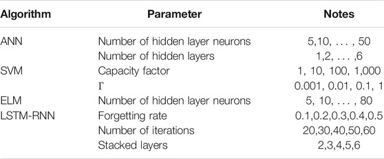
Based on the correlation analysis results, the parameters that are more relevant to the permeability are selected as the input to the machine learning algorithm and then used to predict the permeability. In this study, four algorithms, which are widely used in many fields, were selected to build: ANN, SVM, ELM, and LSTM-RNN. The algorithm principle (Table 1) and operation steps are as follows:

1) ANN

An ANN is a network composed of several neurons, which can process system information by simulating the structure and operating mechanism of the human brain (Das et al., 2014). This algorithm has strong nonlinear approximation ability and fault tolerance and is often used to deal with regression and clustering problems.

The excitation function of the neural network model for permeability prediction constructed in this study selects the sigmoid equation, which is shown in Eq. 5. The model loss function is the mean square error equation, as shown in Eq. 6.

$\text{S}=\frac{1}{1+e^{-t}}(5)$

$\text{C}\left(\text{w},\text{b}\right)\equiv \frac{1}{2n}{{\displaystyle \sum }}_x||\overline{y}-y^2||(6)$

where y is the real permeability, $\overline{y}$ is the permeability generated by the ANN, and w and b are the weights and biases of the algorithm’s hidden layer. In the model training process, the number of hidden layers was set to 1, 2… 6, and the number of neurons was set to 5, 10… 50. The optimal number of hidden layers and the number of neurons in the algorithm were verified using 10-fold cross-validation to determine the best performance.

2) SVM

The purpose of SVM modeling is to find a hyperplane based on the principle of maximum spacing, divide all samples, and simplify the solution to a convex quadratic programming problem. Since the advent of this algorithm (Cortes and Vapnik, 1995), it has shown strong performance in text classification and high-dimensional data processing, which makes it the most widely used machine learning algorithm in many fields (Abdi and Giveki, 2013; Ouyang et al., 2017; Ouyang et al., 2018). The kernel function of the SVM selects the Gaussian radial basis equation:

$\text{K}\left(\text{X},X^{\prime }\right)=\text{exp}\left(\frac{||-\text{X}-X^{\prime }||}{2{\sigma }^2}\right)(7)$

where X is the input data vector, and σ is the standard deviation of the input data. During model training, the algorithm capacity coefficient C is set to 1, 10, 100, and 1,000, and the parameter $\text{γ}=\frac{1}{2{\sigma }^2}$ is set to 0.001,001, 0.1, and 1, and then the optimal parameter combination is determined by 10-fold cross-validation. The model loss function is the mean square error Eq.6.

3) ELM

ELM is a type of single hidden layer feedforward neural network (SLFN). During model training, the algorithm can eliminate the iterative optimization of the input layer weights to the hidden layer and only randomly assign values (Huang et al., 2004; Huang et al., 2006). Therefore, the algorithm has the advantages of a simple mathematical model, fast learning speed, strong generalization ability, and global optimal solutions. At present, the algorithm has been widely used in many fields and has achieved good application results (Li et al., 2018). The solving function of ELM is expressed as follows:

$\text{f}\left(\text{X}\right)={{\displaystyle \sum }}_1^L{\beta }_{l}G\left(a,b,X\right)(8)$

where L is the number of hidden layers of the extreme training machine, a and b are hidden layer node parameters $, {\beta }_l$ is the hidden layer outer weight parameter, and G(∙) is the algorithm excitation function, as shown in Eq. 8. During ELM training, only the number of neurons in the hidden layer must be determined. This parameter was set to 5,10, … ,80, and the optimal parameter was determined by 10-fold cross-validation. The model loss function is the mean square error Eq. 6.

4) LSTM-RNN

LSTM-RNN is a time recursive algorithm based on a recurrent neural network (RNN). Through an in-depth understanding of the global characteristics of the data, it provides the algorithm with more powerful generalization capabilities than other models. Compared with RNN, this algorithm adds a structure of information availability judgment in the training process: the LSTM network (Hochreiter and Schmidhuber, 1997), which consists of input, forgetting, and output gates. When the information flow enters the algorithm network, the redundant information that does not meet the algorithm rules is placed in the forget gate and removed (Li et al., 2021c). In practice, the LSTM-RNN algorithm can be expressed by Eqs 9–13 (Irie et al., 2018):

$i_t=\sigma \left(W_{xi}{x}_t+W_{hi}{h}_{t-1}+W_{ci}{c}_{t-1}+b_i\right)(9)$

$f_t=s\left(W_{xf}{x}_t+W_{hf}{h}_{t-1}+W_{cf}{c}_{t-1}+b_f\right)(10)$

$c_t=f_t{c}_{t-1}+i_t\text{tanh}\left(W_{xc}{x}_t+W_{hc}{h}_{t-1}+b_c\right)(11)$

$o_t=s\left(W_{xo}{x}_t+W_{ho}{h}_{t-1}+W_{co}{c}_{t-1}+b_o\right)(12)$

${\overline{y}}_t=o_t\text{tanh}\left(c_t\right)(13)$

where Wxi, Whi, Wci, Wxf, Whf, Wcf, Wxc, Whc, Wxo, Who, and Wco are the weight parameters of the algorithm excitation function; i_t, f_t, c_t, and o_t are the input gates, forgetting gates, and information judgment status, respectively; and s(∙) is the sigmoid excitation function. In the algorithm training process, the forgetting rate parameter was set to 0.1, 0.2, 0.3, 0.4, and 0.5; the number of iterations parameter was set to 20, 30, 40, 50, 60; and the number of stacking layers was set to 2, 3, 4, 5, and 6. The optimal parameter combination was determined by 10-fold cross-validation. The model loss function is the mean square error Eq. 6.

Error Evaluation Function

To quantitatively evaluate the simulation of the permeability by the selected machine learning algorithm, it is important to analyze the model to predict its performance. Four evaluation functions were chosen in this study: MAE (mean absolute error), MAPE (mean absolute percentage error), RMSE (root mean square error), and MER (max error rate). The evaluation function equations are as follows:

$MAE=\frac{1}{n}{{\displaystyle \sum }}_{t=1}^n\left|{\overline{y}}_t-y_t\right|(14)$

$MAPE=\frac{1}{n}{{\displaystyle \sum }}_{t=1}^n\left|\frac{{\overline{y}}_t-y_t}{y_t}\right|(15)$

$RMSE=\sqrt{\frac{1}{n}{{\displaystyle \sum }}_{t=1}^n{\left({\overline{y}}_t-y_t\right)}^2}(16)$

$MER=\frac{\max \left({\overline{y}}_t-y_t\right)}{y_{MER}}(17)$

where $y_t$ is the real permeability data, ${\overline{y}}_t$ is the calculated permeability data, and $y_{MER}$ is the real permeability data where the maximum error occurs.

By analyzing the four evaluation function equations, MAE can reflect the actual deviation between the real permeability and the calculated value, which can evaluate the dispersion of the algorithm error. MAPE reflects the ratio between the real data and the calculated value, which can evaluate the percentage accuracy of the algorithm, because of the square term. RMSE is more sensitive to large algorithm errors than other evaluations functions. Finally, MER reflects the maximum error ratio, which can be used to evaluate the ability of the algorithm to control the maximum error. It can be seen that the four types of evaluation indicators can evaluate the overall algorithm performance.

Interval Prediction of Permeability

To make the calculated results of permeability prediction more reliable, this study introduces the concept of interval prediction. Interval prediction can reflect the inherent prediction uncertainty and has a high fault-tolerance rate Table 1. The interval prediction in this study is divided into the following three steps.

1) Obtain the absolute value of the true error returned by the optimal algorithm based on the prediction results of the machine learning algorithm.

2) Determine the most suitable probability distribution function type for the error dataset using probability analysis methods.

3) Obtain prediction intervals with different reliabilities based on the point prediction results and probability density function.

TABLE 1

TABLE 1. Parameter selection range in the training process of machine learning algorithms.

Because the permeability error data set is a vector, the process of determining its probability distribution function can be simplified to a fitting problem, in which the data set is substituted into different probability distribution functions, the log likelihood estimation test is used to quantitatively evaluate the fitting effect, and then the fitting function is obtained. In this study, four classical parameter distribution functions were selected: gamma (Eq. 18), lognormal (Eq. 19), exponential (Eq. 20), and Weibull (Eq. 21). Their equations are as follows:

$f\left(\text{x}\right)=\frac{{\left(x/\theta \right)}^{\alpha }{e}^{-x/\theta }}{x\text{τ}\left(\text{α}\right)}(18)$

$f\left(\text{x}\right)=\frac{1}{x\sigma \sqrt{2\pi }}\text{exp}\left(-{\text{z}}^2/2\right)(19)$

$f\left(\text{x}\right)=\frac{e^{-x/\theta }}{\theta }(20)$

$f\left(\text{x}\right)=\frac{\tau {\left(x/\theta \right)}^{\tau }{e}^{-\left(x/{\theta }^{\tau }\right)}}{x}(21)$

where α and θ are the fitting parameters of the gamma distribution, z and σ are the fitting parameters of the lognormal distribution, θ is the fitting parameter of the exponential distribution, and τ and θ are the fitting parameters of the Weibull distribution. Selecting the reliability p to obtain the prediction result of the permeability interval, the equation is as follows:

$\overline{y}\in \left[\text{y}-Va{R}_P\left(y\right),\text{y}+Va{R}_P\left(y\right)\right](22)$

$Va{R}_P\left(X\right)=F_X^{-1}\left(p\right)(23)$

where $F_X^{-1}\left(p\right)$ is the inverse of the cumulative distribution function (CDF) of the probability distribution function and VaR is the threshold corresponding to the distribution function.

Data Collection

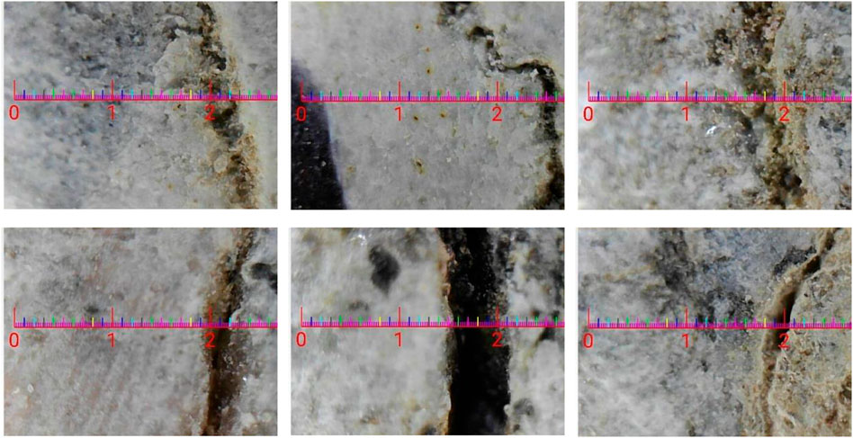
The rock sample was from an actual radioactive waste disposal site in Beishan District, Gansu Province (Figures 1A,B), with no perennial rivers on the surface of the study area, no permanent surface water, and all surface waters formed by seasonal valley flows following intermittent floods. The study area is located in the middle section of the Liuyuan–Tiancang fold belt in the northern Tianshan–Yinshan zonal structural system, which belongs to the Erdaojing–Xiananluzi–Jiusidun north fault fold belt (Figure 2). The chemical composition of major dissolved components of the groundwater in the area is mainly composed of Na-Cl·SO₄, and the groundwater is divided into three main types: bedrock fissure water, basin pore-fissure water, and valley depression fissure-pore water. The lithology of the strata in the area is mainly magmatic rock, mostly granite, which is dominated by medium-fine grained granodiorite, medium-fine grained monzonitic granite, and biotite diorite, all the rockmass are joint developed (Figure 3). As illustrated in Figure 1C, the trend of joints in the study area is mostly northeast to southwest.

FIGURE 1

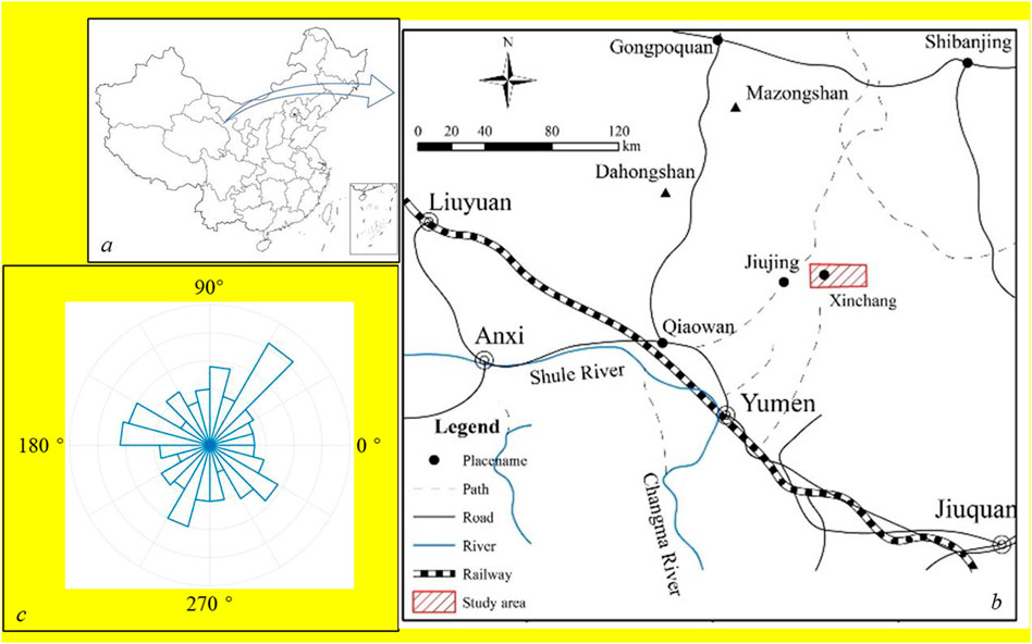
FIGURE 1. Location map of the case study area. (A,B): Location description of study area; (C): The rose diagram of the joins trend.

FIGURE 2

FIGURE 2. Typical fractured rock mass in the study area.

FIGURE 3

FIGURE 3. Width measurement map of partial rock samples (units: mm).

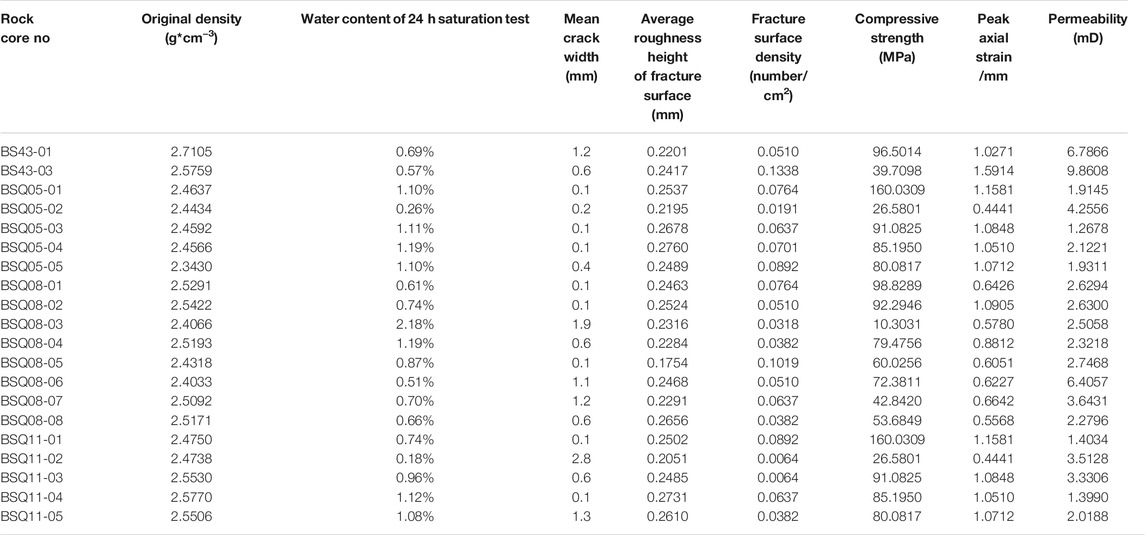
Through on-site sampling, three-dimensional laser scanning, and indoor physical and mechanical tests, the modeling data were obtained, including the original density of the rock sample, average fracture width, average fracture surface roughness height, fracture surface density (the number of cracks per unit area), water content of 24 h saturation test, compressive strength, peak axial strain, and rock sample permeability (Table 2). Additionally, the sample is a standard cylinder with a bottom circle diameter of 50 mm and a height of 100 mm.

TABLE 2

TABLE 2. Modeling data.

Computational Results

Correlation Analysis Results

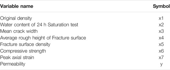
To determine the internal correlation between the case data, it is necessary to obtain the optimal input parameters of the simulation model. First, we performed a correlation analysis on the selected data. To facilitate the description, the variable data were assigned mathematical symbols, and the corresponding relationship is shown in Table 3.

TABLE 3

TABLE 3. Correspondence between variable data and symbols.

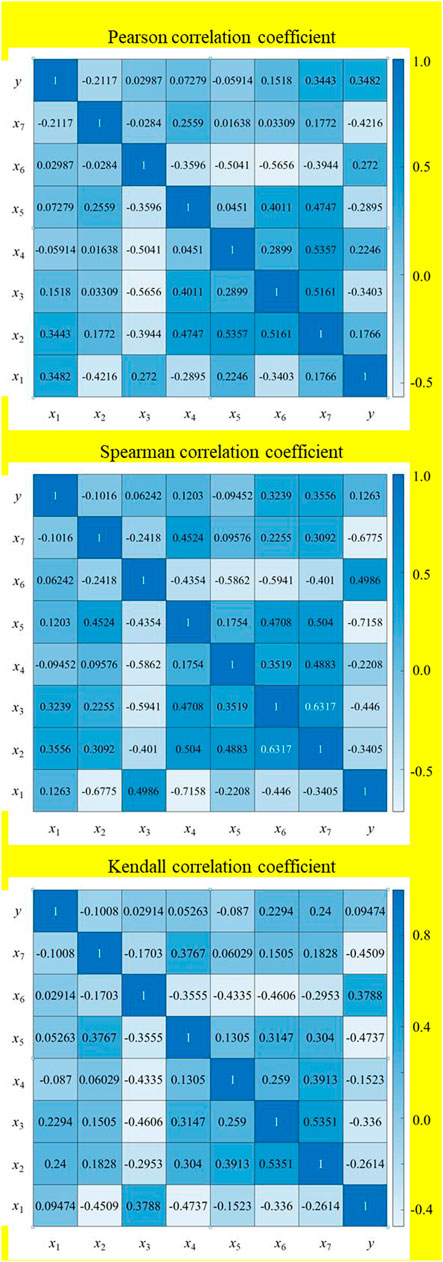
Then, the following parameters were calculated separately: permeability (y), original density (x1), water content of a 24 h water tent saturation test (x2), mean crack width (x3), average rough height of fracture surface (x4), fracture surface density (x5), Pearson correlation coefficient between compressive strength (x6) and peak axial strain (x7), Spearman correlation coefficient, and Kendall correlation coefficient. Among them, the correlation coefficient between permeability and other parameters is used to evaluate the correlation closeness, and the correlation coefficient between other parameters (excluding permeability data) is to eliminate redundant input to simplify the calculation. The results are presented in Figure 4.

FIGURE 4

FIGURE 4. Correlation coefficient results.

It can be seen from Figure 4 that the permeability has the strongest correlation with the water content of the 24 h saturation test, with correlation coefficients of -0.4216, −0.6775, and −0.4509, respectively, which shows the weakest correlation with the original density and the fracture surface density, with correlation coefficients between permeability and original density of 0.3482, 0.1263, and 0.0947, respectively. The ratios of the correlation coefficients between the permeability and fracture surface density were 0.2246, −0.22208, and −0.1523, respectively. Four sets of input parameters were selected to construct the permeability simulation model to reflect the influence of the input parameters scientifically and quantitatively on the simulation results. The parameter combination details are presented in Table 4.

TABLE 4

TABLE 4. Combination of input and output parameters.

Prediction Results

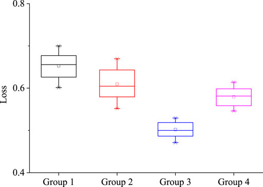
Before building the simulation model, a simple neural network was used to test the fitting performance of the four combinations. The hidden layer of this simple neural network was set to two layers, with twenty neurons in each layer. The obtained data were divided into a training set and a test set according to the ratio of 70 and 30%, and then simulation experiments were conducted on the four combinations, respectively, finally obtaining the loss value when the different combinations converged. To clearly compare the algorithm fitment under different input conditions, this study grouped the loss values once the operation stabilized, and then drew a box diagram, as shown in Figure 5.

FIGURE 5

FIGURE 5. Fitting performance of different input parameters.

Figure 5 shows the returned loss value when the algorithm is stable under different combinations. Among them, the loss value obtained by Group 1 was (0.6001, 0.6969), Group 2 was (0.5534, 0.6697), Group 3 was (0.4705, 0.5282), and Group 4 was (0.5479, 0.6149). The loss value obtained in Group 2 had the largest fluctuation range, up to 0.1166. The loss value obtained in Group 1 was the largest, as its fitting was the worst, while the obtained value in Group 3 was the smallest, and the fluctuation range is also the smallest, only 0.0585. Thus, when Group 3 was used as the input, the fitting effect was the best.

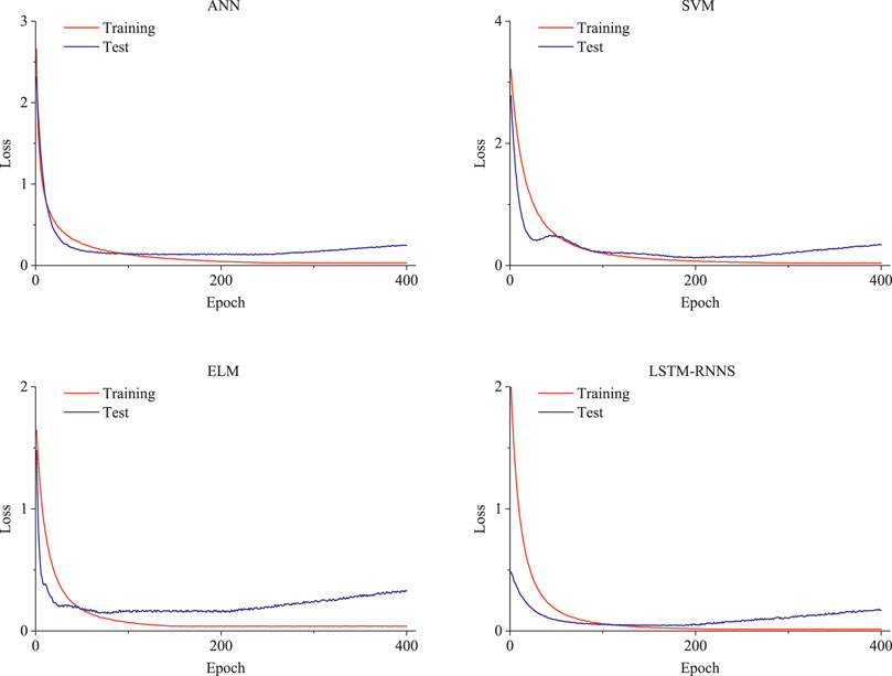
Subsequently, using Group 3 as the input, four methods were selected, including ANN, SVM, ELM, and LSTM-RNN, to construct a simulation model for permeability prediction. In the calculation, the hyper-parameters of all algorithms were adjusted and optimized by cross-validation. Therefore, the relevant connections in the dataset were better investigated. In the training process, the training data set was used to establish the connection between the input and target parameters, and then the test data were used to verify the connection. Figure 6 shows the computational performance of the four algorithms.

FIGURE 6

FIGURE 6. Calculation results of four algorithm loss curves.

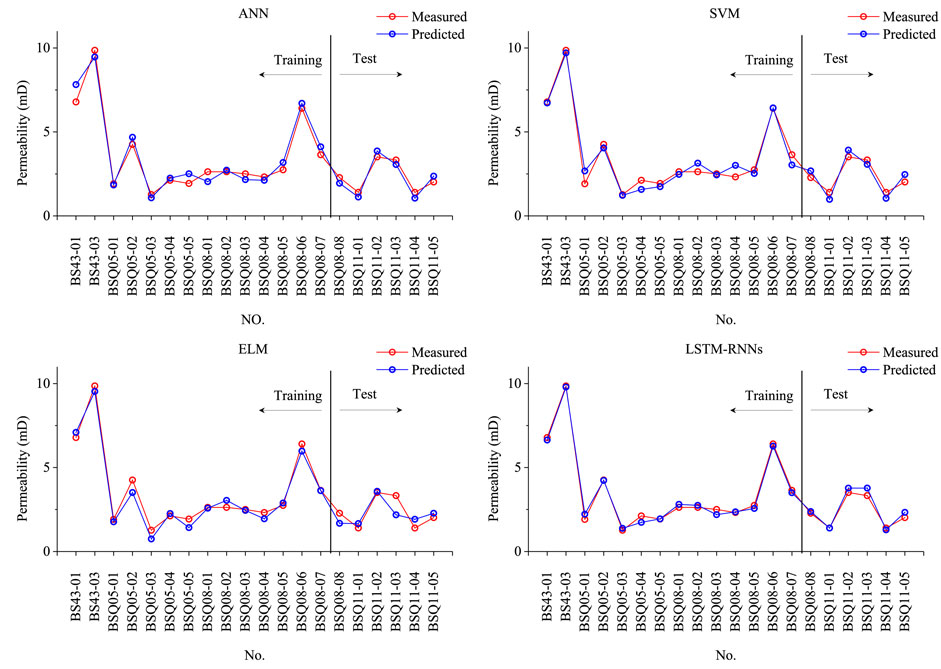
It can be seen from Figure 6 that during training, the algorithm loss decreases as the number of iterations increases. When the number of iterations reached 220, the loss of the ANN algorithm began to converge; for SVM, it was 200 times, for ELM, it was 150 times, and for LSTM-RNN, it was approximately 140 times. Observing the test process, the number of convergence iterations of the four algorithms was less than that of the training process. However, as the number of iterations increased, the training process loss tended to increase slightly. The analysis shows that there was an over-fitting situation at this time. To prevent errors caused by overfitting, this study chose the number of iterations corresponding to the smallest loss value during the test as the final model. That is, when the number of ANN iterations was 256, the loss value of 0.1334 was the smallest. When the number of SVM iterations was 221, its loss reached a minimum of 0.1276. For ELM, when the number of iterations was 191, the loss value was 0.1537. The results are similar for LSTM-RNNs; when the number of iterations was 158, the loss value was only 0.0453. Table 5 summarizes the evaluation indicators of all the algorithm test sets, and Figure 7 shows the final calculation results.

TABLE 5

TABLE 5. Evaluation of the calculation effect of the selected algorithm.

FIGURE 7

FIGURE 7. Summary of calculation results of the four algorithms.

According to Table 5, based on the calculated data, the MAE value obtained by the LSTM-RNN algorithm was only 0.1695, which is smaller than the 0.3337, 0.2962, and 0.3511 for ANN, SVM, and ELM. The MAPE values of the four algorithms were 11.79, 12.64, 14.30, and 6.70%, respectively; the RMSE values were 0.3986, 0.3718, 0.4427, and 0.2102, respectively; and the MER values were 28.19, 39.82, 34.36, and 13.37%, respectively. Thus, the simulation effect of the LSTM-RNN algorithm was the best, and its MAE, MAPE, and RMSE values were only half of those of the other algorithms. Most importantly, the LSTM-RNN algorithm was only 13.37% in the indicator of the largest error in the evaluation of the MER. This means that the difference between the simulated data and real data did not exceed 15%, which reflects the powerful stability and generalizability of the algorithm.

Interval Prediction Results

Based on the comparison calculation, the permeability simulation result was obtained based on the LSTM-RNN algorithm, and the calculation error was also obtained. To make the simulation results more reliable, this study introduced the concept of interval prediction, which increases the fault tolerance of the calculation results. To ensure the generalizability of the interval prediction model, this study first calculated the model training data error, analyzed the probability distribution type of the error generated during the training process, and then extracted the tail thresholds corresponding to different p-values. Finally, the prediction interval was obtained based on this threshold.

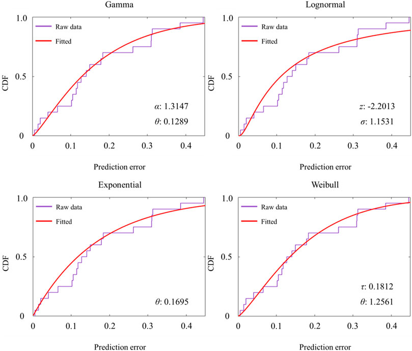
First, it was assumed that the error data in the training phase was normally distributed, and the K-S test was performed (Alexandrowicz and Gula, 2020); however, the calculation result negated this assumption. Subsequently, this study selected four types of widely used non-normal distribution functions to perform the fitting: gamma, lognormal, exponential, and Weibull distributions. The calculation results are shown in Figure 8. Log likelihood (Staude, 2001) was selected as the evaluation index of the fitting situation, which shows that the larger the value, the better the fitting effect. The evaluation results are presented in Table 6.

FIGURE 8

FIGURE 8. Fitting result of forecast error probability distribution.

TABLE 6

TABLE 6. Fitting effect evaluation.

Figure 8 shows the fitting results of the four probability density functions. Combining Eqs 18–21, the fitting parameters of the gamma, lognormal, exponential, and Weibull distributions were 1.3147 and 0.1289, −2.113 and 1.1531, 0.1695, and 0.1812 and 1.2561, respectively. The four probability distribution functions had the best fitting effect under a combination of the above parameters.

Table 6 shows the fitting conditions of the four probability density functions, and the evaluation indicators log likelihood were 15.9286, 13.2983, 15.5004, and 16.1979, respectively. By comparison, it was found that the evaluation index of the Weibull distribution was greater than that of the other three probability density functions, so it can be concluded that the prediction error of permeability is most consistent with the Weibull distribution.

Subsequently, based on the Weibull distribution probability density function and Eq. 23, the VaR values at p-values of 0.90, 0.95, and 0.99 were obtained. The calculation results are presented in Table 7. Finally, the interval simulation results of permeability were obtained based on the simulation results and thresholds of the LSTM-RNNs. The calculation results are shown in Figure 9.

TABLE 7

TABLE 7. Threshold calculation result.

FIGURE 9

FIGURE 9. Simulation results of permeability interval prediction.

It can be seen from Figure 9 that, regardless of the interval simulation under the threshold value, the reliability of the calculation result is better than that of the point value simulation, which gives the algorithm a stronger reliability. When the p-value was 0.90, the interval value was the smallest. As the value of p increased, the simulation interval increased. In summary, when p is 0.90, there are still five points that do not fall within the interval; when p is 0.95, only two points are outside the interval; when p is 0.99, all points fall into the interval, and the reliability reaches up to 100% at this time.

Conclusion

Considering the low-permeability granite body in the study area as the disposal site for high-level radioactive waste, this study focuses on the simulation method of its permeability. To improve the efficiency of permeability acquisition, this study proposed a model structure based on comparing and selecting different machine learning methods, which is different from traditional methods. This method simplifies the acquisition of basic data, optimizes the permeability data calculation steps, and strengthens the reliability of the permeability calculation results. Based on case studies, the main conclusions of this paper are as follows.

1) Based on the correlation analysis, it can be seen that the granite permeability in the case site has the strongest correlation with the water content of the 24 h saturation test, but the weakest correlation with the original density and fracture surface density. Based on this knowledge and machine learning pre-calculation, the input parameters of the permeability simulation model were selected as the original density, saturated water 24 h water content, average crack width, average roughness height of fracture surfaces, compressive strength, and peak axial strain.

2) Based on the ten-fold cross-validation, the computing power of the four machine learning algorithms was optimized, and the respective final calculation results were obtained. The comparison shows that the LSTM-RNN algorithm has the best computational performance, followed by SVM, and then ANN, while ELM has the worst computational performance. Finally, the calculation results of the LSTM-RNN were chosen to perform the interval prediction.

3) Based on the training error of LSTM-RNNs, the probability density function is fitted, and the Weibull distribution fitting effect is concluded to be the best. Therefore, thresholds with p-values of 0.90, 0.95, and 0.99, and the corresponding prediction intervals were obtained. Compared with point value prediction, interval prediction is more reliable.

Data Availability Statement

The original contributions presented in the study are included in the article/Supplementary Material, further inquiries can be directed to the corresponding author.

Author Contributions

NP conceptualized the study, contributed to the study methodology, and wrote the original draft. YW contributed to the study methodology, data curation and investigation. RS and XL contributed to data analysis and investigation. NP and ZW contributed to software and formal analysis. RL and HY contributed to investigation and writing-original draft. All authors have read and agreed to the published version of the manuscript.

Funding

This research is supported by the key program of Sichuan Province (2018JY0425; 2018SZ0290).

Conflict of Interest

The authors declare that the research was conducted in the absence of any commercial or financial relationships that could be construed as a potential conflict of interest.

Publisher’s Note

All claims expressed in this article are solely those of the authors and do not necessarily represent those of their affiliated organizations, or those of the publisher, the editors, and the reviewers. Any product that may be evaluated in this article, or claim that may be made by its manufacturer, is not guaranteed or endorsed by the publisher.

References

Abdi, M. J., and Giveki, D. (2013). Automatic Detection of Erythemato-Squamous Diseases Using PSO-SVM Based on Association Rules. Eng. Appl. Artif. Intell. 26 (1), 603–608. doi:10.1016/j.engappai.2012.01.017

CrossRef Full Text | Google Scholar

Alexandrowicz, R. W., and Gula, B. (2020). Comparing Eight Parameter Estimation Methods for the Ratcliff Diffusion Model Using Free Software. Front. Psychol. 11, 484737. doi:10.3389/fpsyg.2020.484737

PubMed Abstract | CrossRef Full Text | Google Scholar

Cao, R.-h., and Lin, H. (2017). Experimental and Numerical Study of Failure Behavior and Energy Mechanics of Rock-like Materials Containing Multiple Joints. Adv. Mater. Sci. Eng. 2017, 1–17. doi:10.1155/2017/6460150

CrossRef Full Text | Google Scholar

Chapman, N., and Hooper, A. (2012). The Disposal of Radioactive Wastes Underground. Proc. Geologists' Assoc. 123 (1), 46–63. doi:10.1016/j.pgeola.2011.10.001

CrossRef Full Text | Google Scholar

Cortes, C., and Vapnik, V. (1995). Support-vector Networks. Mach Learn. 20 (3), 273–297. doi:10.1007/bf00994018

CrossRef Full Text | Google Scholar

Das, G., Pattnaik, P. K., and Padhy, S. K. (2014). Artificial Neural Network Trained by Particle Swarm Optimization for Non-linear Channel Equalization. Expert Syst. Appl. 41 (7), 3491–3496. doi:10.1016/j.eswa.2013.10.053

CrossRef Full Text | Google Scholar

Deo, R. C. (2015). Machine Learning in Medicine. Circulation 132 (20), 1920–1930. doi:10.1161/circulationaha.115.001593

PubMed Abstract | CrossRef Full Text | Google Scholar

Esteves, J. T., de Souza Rolim, G., and Ferraudo, A. S. (2019). Rainfall Prediction Methodology with Binary Multilayer Perceptron Neural Networks. Clim. Dyn. 52 (3-4), 2319–2331. doi:10.1007/s00382-018-4252-x

CrossRef Full Text | Google Scholar

Gessulat, S., Schmidt, T., Zolg, D. P., Samaras, P., Schnatbaum, K., Zerweck, J., et al. (2019). Prosit: Proteome-wide Prediction of Peptide Tandem Mass Spectra by Deep Learning. Nat. Methods 16 (6), 509–518. doi:10.1038/s41592-019-0426-7

PubMed Abstract | CrossRef Full Text | Google Scholar

Hadgu, T., Karra, S., Kalinina, E., Makedonska, N., Hyman, J. D., Klise, K., et al. (2017). A Comparative Study of Discrete Fracture Network and Equivalent Continuum Models for Simulating Flow and Transport in the Far Field of a Hypothetical Nuclear Waste Repository in Crystalline Host Rock. J. Hydrol. 553, 59–70. doi:10.1016/j.jhydrol.2017.07.046

CrossRef Full Text | Google Scholar

He, Y., and Kusiak, A. (2018). Performance Assessment of Wind Turbines: Data-Derived Quantitative Metrics. IEEE Trans. Sustain. Energ. 9 (1), 65–73. doi:10.1109/tste.2017.2715061

CrossRef Full Text | Google Scholar

He, Y., Kusiak, A., Ouyang, T., and Teng, W. (2017). Data-driven Modeling of Truck Engine Exhaust Valve Failures: A Case Study. J. Mech. Sci. Technol. 31 (6), 2747–2757. doi:10.1007/s12206-017-0518-1

CrossRef Full Text | Google Scholar

Hochreiter, S., and Schmidhuber, J. (1997). Long Short-Term Memory. Neural Comput. 9 (8), 1735–1780. doi:10.1162/neco.1997.9.8.1735

PubMed Abstract | CrossRef Full Text | Google Scholar

Huang, G. B., Zhu, Q. Y., and Siew, C. K. (2004). Extreme Learning Machine: a New Learning Scheme of Feedforward Neural Networks. Neural Networks 2, 985–990. doi:10.1109/IJCNN.2004.1380068

CrossRef Full Text | Google Scholar

Huang, G. B., Zhu, Q. Y., and Siew, C. K. (2006). Extreme Learning Machine: Theory and Applications. Neurocomputing 70 (1-3), 489–501. doi:10.1016/j.neucom.2005.12.126

CrossRef Full Text | Google Scholar

Irie, K., Lei, Z., Schlüter, R., and Ney, H. (2018). “Prediction of LSTM-RNN Full Context States as a Subtask for N-Gram Feedforward Language Models,” in 2018 IEEE International Conference on Acoustics, Speech and Signal Processing (ICASSP), Calgary, AB, April 15–20, 2018 (IEEE), 6104–6108.

CrossRef Full Text | Google Scholar

Jiang, Q., Ye, Z., and Zhou, C. (2014). A Numerical Procedure for Transient Free Surface Seepage through Fracture Networks. J. Hydrol. 519, 881–891. doi:10.1016/j.jhydrol.2014.07.066

CrossRef Full Text | Google Scholar

Khoei, A. R., Hosseini, N., and Mohammadnejad, T. (2016). Numerical Modeling of Two-phase Fluid Flow in Deformable Fractured Porous media Using the Extended Finite Element Method and an Equivalent Continuum Model. Adv. Water Resour. 94, 510–528. doi:10.1016/j.advwatres.2016.02.017

CrossRef Full Text | Google Scholar

Lai, J., Wang, G., Fan, Z., Chen, J., Qin, Z., Xiao, C., et al. (2017). Three-dimensional Quantitative Fracture Analysis of Tight Gas Sandstones Using Industrial Computed Tomography. Sci. Rep. 7 (1), 1825. doi:10.1038/s41598-017-01996-7

PubMed Abstract | CrossRef Full Text | Google Scholar

Li, B., Wong, R. C. K., and Milnes, T. (2014). Anisotropy in Capillary Invasion and Fluid Flow through Induced sandstone and Shale Fractures. Int. J. Rock Mech. Mining Sci. 65, 129–140. doi:10.1016/j.ijrmms.2013.10.004

CrossRef Full Text | Google Scholar

Li, H., Xu, Q., He, Y., and Deng, J. (2018). Prediction of Landslide Displacement with an Ensemble-Based Extreme Learning Machine and Copula Models. Landslides 15 (10), 2047–2059. doi:10.1007/s10346-018-1020-2

CrossRef Full Text | Google Scholar

Li, H., Xu, Q., He, Y., Fan, X., and Li, S. (2020). Modeling and Predicting Reservoir Landslide Displacement with Deep Belief Network and EWMA Control Charts: a Case Study in Three Gorges Reservoir. Landslides 17 (3), 693–707. doi:10.1007/s10346-019-01312-6

CrossRef Full Text | Google Scholar

Li, H., Deng, J., Feng, P., Pu, C., Arachchige, D. D. K., and Cheng, Q. (2021a). Short-Term Nacelle Orientation Forecasting Using Bilinear Transformation and ICEEMDAN Framework. Front. Energ. Res. 9, 780928. doi:10.3389/fenrg.2021.780928

CrossRef Full Text | Google Scholar

Li, H., Deng, J., Yuan, S., Feng, P., and Arachchige, D. D. K. (2021b). Monitoring and Identifying Wind Turbine Generator Bearing Faults Using Deep Belief Network and EWMA Control Charts. Front. Energ. Res. 9, 799039. doi:10.3389/fenrg.2021.799039

CrossRef Full Text | Google Scholar

Li, H., Xu, Q., He, Y., Fan, X., Yang, H., and Li, S. (2021c). Temporal Detection of Sharp Landslide Deformation with Ensemble-Based LSTM-RNNs and Hurst Exponent. Geomatics, Nat. Hazards Risk 12 (1), 3089–3113. doi:10.1080/19475705.2021.1994474

CrossRef Full Text | Google Scholar

Longoni, L., Arosio, D., Scaioni, M., Papini, M., Zanzi, L., Roncella, R., et al. (2012). Surface and Subsurface Non-invasive Investigations to Improve the Characterization of a Fractured Rock Mass. J. Geophys. Eng. 9 (5), 461–472. doi:10.1088/1742-2132/9/5/461

CrossRef Full Text | Google Scholar

Ning, Y., Yang, J., An, X., and Ma, G. (2011). Modelling Rock Fracturing and Blast-Induced Rock Mass Failure via Advanced Discretisation within the Discontinuous Deformation Analysis Framework. Comput. Geotechn. 38 (1), 40–49. doi:10.1016/j.compgeo.2010.09.003

CrossRef Full Text | Google Scholar

Ouyang, T., Kusiak, A., and He, Y. (2017). Predictive Model of Yaw Error in a Wind Turbine. Energy 123, 119–130. doi:10.1016/j.energy.2017.01.150

CrossRef Full Text | Google Scholar

Ouyang, T., He, Y., and Huang, H. (2018). Monitoring Wind Turbines’ Unhealthy Status: a Data-Driven Approach. IEEE Trans. Emerging Top. Comput. Intell. 3 (2), 163–172. doi:10.1109/TETCI.2018.2872036

CrossRef Full Text | Google Scholar

Ouyang, T., He, Y., Li, H., Sun, Z., and Baek, S. (2019). Modeling and Forecasting Short-Term Power Load with Copula Model and Deep Belief Network. IEEE Trans. Emerg. Top. Comput. Intell. 3 (2), 127–136. doi:10.1109/tetci.2018.2880511

CrossRef Full Text | Google Scholar

Patterson, J. W., Driesner, T., Matthai, S., and Tomlinson, R. (2018). Heat and Fluid Transport Induced by Convective Fluid Circulation within a Fracture or Fault. J. Geophys. Res. Solid Earth 123 (4), 2658–2673. doi:10.1002/2017jb015363

CrossRef Full Text | Google Scholar

Ren, F., Ma, G., Fu, G., and Zhang, K. (2015). Investigation of the Permeability Anisotropy of 2d Fractured Rock Masses. Eng. Geol. 196, 171–182. doi:10.1016/j.enggeo.2015.07.021

CrossRef Full Text | Google Scholar

Staude, G. H. (2001). Precise Onset Detection of Human Motor Responses Using a Whitening Filter and the Log-Likelihood-Ratio Test. IEEE Trans. Biomed. Eng. 48 (11), 1292–1305. doi:10.1109/10.959325

PubMed Abstract | CrossRef Full Text | Google Scholar

Xu, Q., Li, H., He, Y., Liu, F., and Peng, D. (2019). Comparison of Data-Driven Models of Loess Landslide Runout Distance Estimation. Bull. Eng. Geol. Environ. 78 (2), 1281–1294. doi:10.1007/s10064-017-1176-3

CrossRef Full Text | Google Scholar

Yao, Y. (2012). Linear Elastic and Cohesive Fracture Analysis to Model Hydraulic Fracture in Brittle and Ductile Rocks. Rock Mech. Rock Eng. 45 (3), 375–387. doi:10.1007/s00603-011-0211-0

CrossRef Full Text | Google Scholar

Zhang, Y., Xu, M., Li, X., Qi, J., Zhang, Q., Guo, J., et al. (2018). Hydrochemical Characteristics and Multivariate Statistical Analysis of Natural Water System: A Case Study in Kangding County, Southwestern China. Water 10 (1), 80. doi:10.3390/w10010080

CrossRef Full Text | Google Scholar

Zhang, Y., Dai, Y., Wang, Y., HuangXiao, X. Y., Xiao, Y., and Pei, Q. (2021a). Hydrochemistry, Quality and Potential Health Risk Appraisal of Nitrate Enriched Groundwater in the Nanchong Area, Southwestern China. Sci. Total Environ. 784, 147186. doi:10.1016/j.scitotenv.2021.147186

PubMed Abstract | CrossRef Full Text | Google Scholar

Zhang, Y., He, Z., Tian, H., Huang, X., Zhang, Z., Liu, Y., et al. (2021b). Hydrochemistry Appraisal, Quality Assessment and Health Risk Evaluation of Shallow Groundwater in the Mianyang Area of Sichuan Basin, Southwestern China. Environ. Earth Sci. 80 (17), 576. doi:10.1007/s12665-021-09894-y

CrossRef Full Text | Google Scholar

Zhou, Q., Salve, R., Liu, H. H., Wang, J. S., and Hudson, D. (2006). Analysis of a Mesoscale Infiltration and Water Seepage Test in Unsaturated Fractured Rock: Spatial Variabilities and Discrete Fracture Patterns. J. Contam. Hydrol. 87 (1-2), 96–122. doi:10.1016/j.jconhyd.2006.05.001

CrossRef Full Text | Google Scholar