A New Fluid Mobility Calculation Method Based on Frequency-Dependent AVO Inversion

Fluid mobility (i.e., permeability to viscosity ratio) is a key parameter that can evaluate the reservoir permeability and delineate the fluid characteristic in hydrocarbon-saturated reservoirs. Based on the asymptotic representation for the frequency-dependent reflections in the fluid-saturated pore-elastic media and frequency-dependent AVO inversion, we propose a novel method for estimating fluid mobility from poststack seismic data. First, we establish the relationship between fluid mobility and frequency-dependent AVO analysis. Then, the fluid mobility is estimated using the theory of frequency-dependent AVO inversion. Tests on synthetic data reveal that the fluid mobility shows excellent imageability for the fluid-saturated reservoirs and can accurately delineate the spatial distribution shape of the gas-saturated reservoir. The application of field data examples demonstrates that the fluid mobility calculated by the proposed method produces less background interferences caused by elastic layers compared with the conventional frequency-dependent fluid indicator. The frequency-dependent fluid mobility takes into account the dispersion features associated with hydrocarbon reservoirs, and it provides a new way to detect the location of hydrocarbon reservoirs and characterize their spatial distribution.

Introduction

The reservoir permeability is a key parameter for measuring the capacity of fluid flow in porous rock and it is commonly measured through laboratory experiments. The poroelasticity theory indicates that permeability is significantly related to the seismic attenuation induced by the fluid flow when seismic waves penetrate the hydrocarbon-bearing reservoirs (Biot, 1956a; Biot, 1956b). Many studies have demonstrated that the seismic response of reservoirs is closely dependent on permeability (Pride et al., 2003; Kozlov, 2007; Goloshubin et al., 2008; Rubino et al., 2012). However, estimating permeability from real seismic data is a challenge for reservoir geophysicists until now, especially for the data without well data constraints. Fluid mobility (i.e., permeability to viscosity ratio) can reflect the reservoir permeability and fluid flow behaviors in a porous rock simultaneously and can be extracted from the surface seismic data, which provides an indirect factor to evaluate the percolation properties of a porous media (Rusakov et al., 2016). The measurement and numerical simulation illustrate that fluid mobility is a key parameter that can directly affect the seismic responses associated with the hydrocarbon-saturated reservoirs (Batzle et al., 2006; Goloshubin et al., 2008; Chen et al., 2013a; Ren et al., 2013). The seismic reflection coefficient obtained by the theory of asymptotic representation for the reflection of a seismic wave from a fluid-saturated porous medium provides a basic theory for estimating fluid mobility (Silin et al., 2006; Silin and Goloshubin, 2010). Based on this asymptotic analysis theory, the fluid mobility calculation method using the low-frequency information of the seismic spectrum is proposed by Chen et al. (2012). Further, Chen et al. (2013a) delineated the gas reservoirs and their spatial distribution by integrating the low-frequency shadow and fluid mobility, which greatly reduced the uncertainty of reservoir prediction. In recent years this technology has emerged as a particularly attractive candidate for reservoir prediction. Luo et al. (2018) proposed an integrated prediction strategy for reservoir prediction using the seismic inversion and fluid mobility attribute. Because the fluid mobility calculation is dependent on the time-frequency analysis method, the arrival of new time-frequency transform methods has shown an improvement in spatial resolution of the fluid mobility. Xue et al. (2018) employed the synchrosqueezed wavelet transforms to improve the estimation precision of fluid mobility. Zhang et al. (2020) further use fluid mobility to predict the high-quality reservoir based on a modified high-precision time-frequency transform. These studies illustrate that reservoir-related fluid mobility is a key attribute for reservoir delineation. However, the calculation of these methods mentioned above only uses the seismic information of a single frequency in a low-frequency range and ignores frequency-dependent behaviors associated with the hydrocarbon reservoirs. In the paper, these methods that use the low-frequency information of seismic data for calculating fluid mobility are uniformly defined as the LF-FM. The fluid mobility extracted by the LF-FM commonly indicates the location of the reservoir interface. Therefore, this study is focused on further extracting the fluid mobility from frequency-dependent seismic data to obtain the fluid mobility between the reservoir interfaces.

It is commonly known that the calculation formula of fluid mobility proposed by Chen et al. (2012) is frequency-dependent. So extracting the fluid mobility using frequency-dependent information of seismic data is of great importance for reservoir delineation. Evidence from several studies indicated that the frequency-dependent seismic responses induced by the velocity dispersion and amplitude attenuation occur when the seismic waves pass through the hydrocarbon saturated porous rocks (Chapman et al., 2003; Batzle et al., 2006; Chapman et al., 2006; Gurevich et al., 2010; Dupuy and Stovas, 2013; Chen et al., 2016; Qin et al., 2018). Frequency-dependent effects associated with hydrocarbon-bearing reservoirs provide theoretical supports for computing reservoir-related attributes using seismic data. The frequency-dependent AVO (FDAVO) inversion method provides an approach to estimate the dispersion attribute for reservoir delineation (Wilson et al., 2009; Wu et al., 2012; Chen et al., 2014; Liu et al., 2019; Wang et al., 2019; Luo et al., 2020; Jin et al., 2021). Therefore, the FDAVO inversion is being explored to extract fluid mobility using the frequency-dependent information of seismic data.

In this paper, based on the theory of asymptotic representation of frequency-dependent reflection in the fluid-saturated medium and FDAVO inversion method, we first established the relationship between fluid mobility and FDAVO. And then, the fluid mobility calculation method using frequency-dependent information of post-stack seismic data is proposed. Next, a synthetic data test is used to verify the effectiveness of the proposed approach. Finally, field data examples are further analyzed to illustrate the feasibility of the proposed method.

Theory and Method

Based on the low-frequency asymptotic analysis theory, Chen et al. (2012) derived the expression of reservoir fluid mobility:

$F=\frac{\kappa }{\eta }=\frac{1}{C^2}{\left(\frac{dR}{d\omega }\right)}^2\omega (1)$

where k is the reservoir permeability, η denotes the fluid viscosity, R is the reflection coefficient of a planar compression wave from the interface between elastic and fluid-saturated porous media, ω denotes the angular frequency, parameter C is a function of the bulk density and can be regarded as a constant.

Wilson et al. (2009) and Wu et al. 2010, Wu et al., 2012) extended the two-term AVO linear approximation proposed by Smith and Gidlow (1987) to frequency domain. The frequency-dependent reflection coefficient has the following form

$R\left(\theta ,\omega \right)\approx A\left(\theta \right)\frac{\Delta v_p}{v_p}\left(\omega \right)+B\left(\theta \right)\frac{\Delta v_s}{v_s}\left(\omega \right)(2)$

where θ is incident angle, v_p and v_s with the units of m/s represent P-wave velocity and S-wave velocity, respectively. The expressions of $A\left(\theta \right)$ and $B\left(\theta \right)$ are as follows:

$A\left(\theta \right)=\frac{5}{8}-\frac{1}{2}\frac{v_s^2}{v_p^2}{\sin }^2\theta +\frac{1}{2}{\tan }^2\theta ,B\left(\theta \right)=-4\frac{v_s^2}{v_p^2}{\sin }^2\theta (3)$

Due to the reflection coefficient R in Eq. 1 is the normal reflection of a compression wave, we let $\theta =0$ to pursue a simplified version of Eq. 2 that is an approximation of the normal reflection coefficient. Then, we obtain

$R\left(\omega \right)\approx \frac{5}{8}\frac{\Delta v_p}{v_p}\left(\omega \right)(4)$

Taking the derivative of Eq. 4 with respect to the angular frequency ω, we obtain

$\frac{dR}{d\omega }\approx \frac{5}{8}\frac{d}{d\omega }\left(\frac{\Delta v_p}{v_p}\right)(5)$

By virtue of Eqs 1, 5, we can get the new frequency-dependent expression of the fluid mobility:

$F\left(\omega \right)\approx P^2{\left[\frac{d}{d\omega }\left(\frac{\Delta v_p}{v_p}\right)\right]}^2\omega (6)$

where P is a new constant with $P=\frac{5}{8C}$. Here, the parameter P can be regarded as a scale factor. Therefore, the Eq. 6 can be further rewritten as:

$F\left(\omega \right)\approx \omega {\left[\frac{d}{d\omega }\left(\frac{\mathrm{\Delta }{v}_p}{v_p}\right)\right]}^2(7)$

Expanding Eq. 4 as first-order Taylor series at a reference frequency ω₀ without considering the higher-order terms, we can get:

$R\left(\omega \right)\approx \frac{5}{8}\frac{\mathrm{\Delta }{v}_p}{v_p}\left({\omega }_0\right)+\left(\omega -{\omega }_0\right)\frac{5}{8}\frac{d}{d\omega }\left(\frac{\mathrm{\Delta }{v}_p}{v_p}\right)(8)$

In general, the value of ω₀ is determined by the spectral decomposition and the dominant frequency of the seismic signal is usually selected as the reference frequency.

By virtue of Eqs 7, 8, we can obtain a new expression of frequency-dependent reflection coefficient relating to the fluid mobility, that is:

$R\left(\omega \right)\approx \frac{5}{8}\frac{\mathrm{\Delta }{v}_p}{v_p}\left({\omega }_0\right)+\frac{5}{8}\frac{\left(\omega -{\omega }_0\right)}{\omega }\frac{1}{D_p}F\left(\omega \right)(9)$

where, D_p represents the derivatives of frequency-dependent velocity of P-wave and its expression is $D_p=\frac{d}{d\omega }\left(\frac{\mathrm{\Delta }{v}_p}{v_p}\right)$.

Eq. 8 can be further rewritten as:

$R\left(\omega \right)-\frac{5}{8}\frac{\mathrm{\Delta }{v}_p}{v_p}\left({\omega }_0\right)\approx \frac{5}{8}\frac{\left(\omega -{\omega }_0\right)}{\omega }\frac{1}{D_p}F\left(\omega \right)(10)$

Considering m angular frequencies [ω₁, ω₂, …, ω_m], the vectors r and e can be expressed in matrix form:

$\mathbf{r}=\left[\begin{array}{c}R\left(t,{\omega }_1\right)-\frac{5}{8}\frac{\mathrm{\Delta }{v}_p}{v_p}\left({\omega }_0\right)\\ ⋮\\ R\left(t,{\omega }_m\right)-\frac{5}{8}\frac{\mathrm{\Delta }{v}_p}{v_p}\left({\omega }_0\right)\end{array}\right](11)$

$\mathbf{e}=\left[\begin{array}{c}\frac{5}{8}\frac{\left({\omega }_1-{\omega }_0\right)}{{\omega }_1}\frac{1}{D_p}\\ ⋮\\ \frac{5}{8}\frac{\left({\omega }_m-{\omega }_0\right)}{{\omega }_m}\frac{1}{D_p}\end{array}\right](12)$

Then, we obtain:

$\mathbf{r}=\mathbf{e}F(13)$

At last, the least-squares inversion method can be used to estimate the frequency-dependent fluid mobility F:

$F={\left({\mathbf{e}}^{{\rm T}}\mathbf{e}\right)}^{-1}{\mathbf{e}}^{{\rm T}}\mathbf{r}(14)$

where the T indicates the transpose of the matrix.

In the Eq. 10, the D_p is also calculated by the least-squares inversion method:

$D_p={\left({\mathbf{d}}^{{\rm T}}\mathbf{d}\right)}^{-1}{\mathbf{d}}^{{\rm T}}\mathbf{r}(15)$

where, the form of vector d is:

$\mathbf{d}=\left[\begin{array}{c}\frac{5}{8}\left({\omega }_1-{\omega }_0\right)\\ ⋮\\ \frac{5}{8}\left({\omega }_m-{\omega }_0\right)\end{array}\right](16)$

To extract the frequency-dependent information from the reflected seismic waves, the time-frequency decomposition method is used in the fluid mobility inversion. The seismic reflection amplitude $R\left(t\right)$ can be transformed into data sets $S\left(t,f\right)$ at different frequencies using generalized S-transform (GST) (Chen et al., 2009), that is

$R\left(t\right)\stackrel{GST}{\to }S\left(t,f\right)(17)$

where, the expression of GST is:

$S\left(f,\tau \right)={\displaystyle {\int }_{-\infty }^{+\infty }x\left(t\right)\frac{\left|\lambda \right|{\left|f\right|}^p}{\sqrt{2\pi }}\exp \left[-\frac{{\lambda }^2{\left(t-\tau \right)}^2{f}^{2p}}{2}\right]}\exp \left(-i2\pi ft\right)dt(18)$

where x(t) is the original seismic signal, τ is the time shift parameter, λ and p are the adjustable parameters and control the Gaussian window, S(f, τ) is the expression of a 2D time-frequency variable with regard to f and τ.

The Application to Synthetic and Field Data Examples

Synthetic Data Test

To illustrate the effectiveness of the proposed method, we design a simple gas-saturated permeable reservoir model (Figure 1A) to test the feasibility of the frequency-dependent fluid mobility to delineate reservoirs. In the model, the gas-saturated reservoir is marked with ③, and other layers are dry strata. The black curve indicates the reservoir location. The model parameters are given in Table 1. We perform the forward modeling and migration to produce the synthetic seismic records (Figure 1B) by employing the DVWE (diffusive and viscous wave equation)-based method (He et al., 2008; Chen et al., 2013b; Chen et al., 2016). In the modeling, the frequency-dependent velocity of the gas-saturated reservoir is calculated by the theory proposed by Chapman et al. (2003). The synthetic seismic records were generated using a Ricker wavelet with the dominant frequency of 40 Hz. The seismic records shown in Figure 1B indicate that the top interface of gas-saturated reservoir show strong seismic reflection anomalies. However, the seismic reflections of the reservoir bottom interface show obviously time delay and phase distortion. Besides, the seismic reflections at the bottom of the gas-saturated sand reservoir show noticeable amplitude attenuation and phase delay due to the seismic effects of velocity dispersion.

FIGURE 1

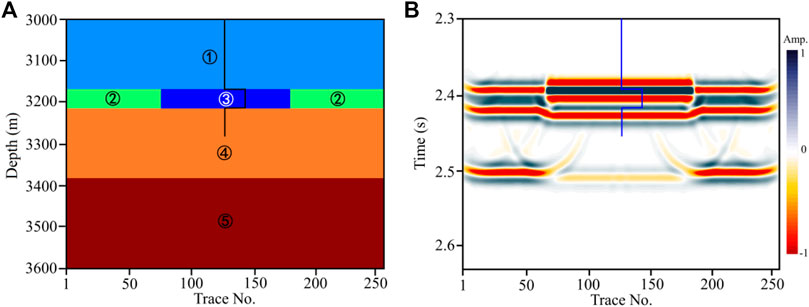
FIGURE 1. (A) The gas-saturated permeable sand reservoir model and (B) its synthetic seismic section.

TABLE 1

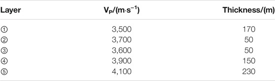
TABLE 1. Physical parameters used in the modeling.

Then, we calculate the frequency-dependent fluid mobility of the model using the proposed method and compare it with the result of LF-FM, and the estimation results are shown in Figure 2. As shown in Figure 2A, the high value of fluid mobility calculated by the LF-FM indicates the top interface rather than the actual spatial distribution shape of the gas-saturated reservoir. However, in Figure 2B, the fluid mobility estimated using our method shows clear anomalies in the reservoir region and the gas storage space correlates well with the reservoir shape. The test for the synthetic data illustrates that the fluid mobility calculated by the frequency-dependent inversion method can accurately delineate the location of the gas-saturated reservoir.

FIGURE 2

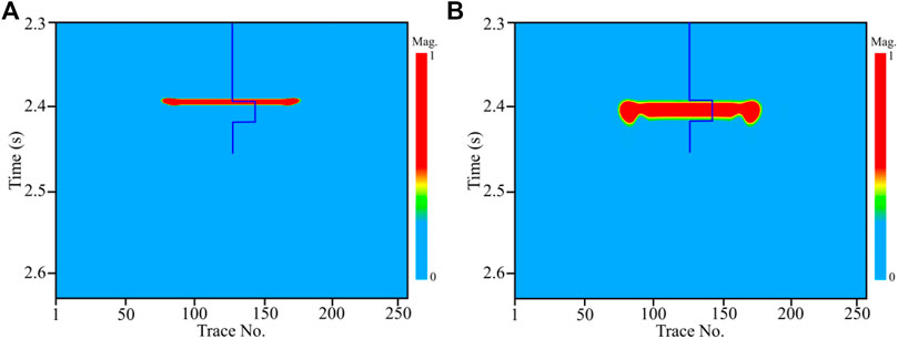
FIGURE 2. The fluid mobility sections calculated by (A) the LF-FM method and (B) our method.

To further analyze the influence of the tuning effect on the fluid mobility calculation, we also make a model (Figure 3A) with thickness of the gas-saturated reservoir less than a quarter wavelength. In the new model, the reservoir thickness is 20 m, and other parameters are the same to the model shown in Figure 1A. The synthetic seismic record (Figure 3B) indicates that the reflection interfaces of the thin reservoir are difficult to distinguish from the seismic events due to the tuning effect. As can be seen in Figures 3C,D, the fluid mobility calculated by the LF-FM and our method can both accurately delineate the reservoir location and its shape.

FIGURE 3

FIGURE 3. (A) The gas-saturated reservoir model with the reservoir thickness is 20 m and (B) its synthetic seismic record. The fluid mobility calculated by (C) LF-FM and (D) our method.

Field Data Applications

In this section, we apply the proposed method to field seismic data to further demonstrate the performance of the proposed method. The reservoirs in the study area are mainly marine sandstone reservoirs with different gas saturations. Figure 4 shows the two well-logs through the sandstone reservoirs, including water saturation (S_w), P-wave, S-wave, density and porosity curves. As shown in Figure 4, the velocities of S-wave show high values in the third column and the porosity in the reservoir zones is about 18%. However, compared to the non-reservoir zones, the velocity curves of P-wave in the second column and the density curves in the fourth column are both show a change to lower values. The reservoirs with high gas saturation are outlined by cyan rectangles. We choose two seismic profiles across the two wells for analysis. The seismic profile shown in Figure 5A intersecting well-1 is extracted from the line marked with M to M’ in a three-dimensional (3D) area. Figure 5B is the seismic trace extracted at the well-1 location (CDP No.178) and Figure 5C is its time-frequency spectrum after the GST. In the Figure 5C, we can observe strong energy at the reservoir zone. The section shown in Figure 5D intersecting well-2 is extracted from the line marked with N to N’. Figure 5E is the seismic trace extracted at the well-2 location (CDP No.146) and Figure 5F is its time-frequency spectrum after the GST. In Figure 5F, there are two strong energy clusters in the reservoir zone. The amplitude spectra shown in Figures 5G,H of the two seismic traces (Figures 5B,E) illustrate that the frequency band is approximately 5–50 Hz, and the dominant frequency is about 20 Hz.

FIGURE 4

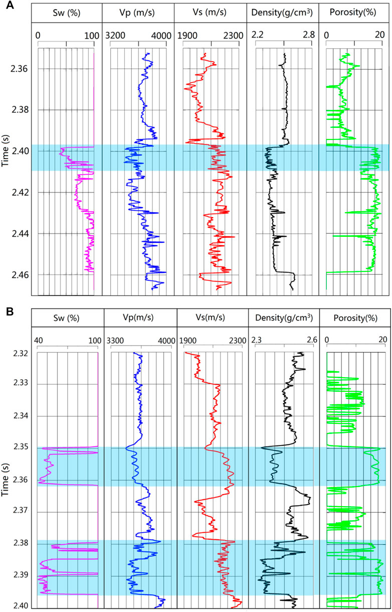
FIGURE 4. Well logs of the sandstone reservoir for (A) well-1 and (B) well-2. The reservoir in the study area is gas-saturated sandstone and the cyan rectangle outlines the fluid-saturated reservoirs saturated with high gas saturation (Sg ≥ 0.4).

FIGURE 5

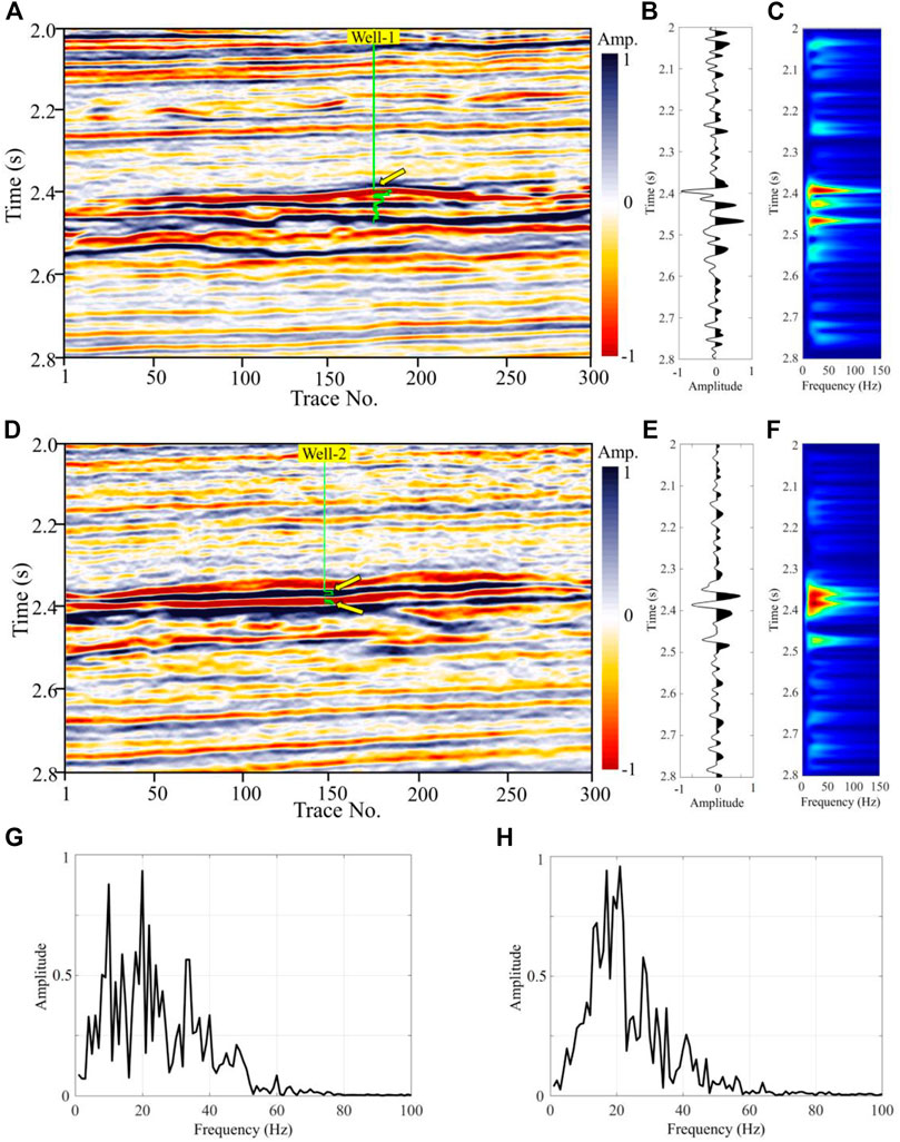
FIGURE 5. (A) The stacked section across the Well-1. (B) The seismic trace extracted at the Well-1 location and (C) its time-frequency spectrum calculated by GST. (D) The stacked section across the Well-2. (E) The seismic trace extracted at the Well-2 location and (F) its time-frequency spectrum calculated by GST. (G) and (H) are the amplitude spectra of Figures 5B,E, respectively. In the two sections, the reservoir zones are indicated with the yellow arrows.

To evaluate the ability for imaging the reservoirs, we calculated the fluid mobility of the two seismic sections and compared it with the dispersion attribute of P-wave obtained by frequency-dependent AVO inversion (Wilson et al., 2009; Wu et al., 2012; Chen et al., 2014; Luo et al., 2020). The comparison results are shown in Figure 6. For the results of the section across the Well-1, the dispersion attribute (Figure 6A) delineates the reservoir zone while the results are greatly affected by the other anomalies. However, the fluid mobility result in Figure 6B shows a high value at the location of the reservoir zone and the background interference unrelated to the reservoirs are very weak. For the results of the section across the Well-2, the result of dispersion attribute (Figure 6C) of P-wave is also affected by the other interference, which results in difficulty for accurately discriminating the reservoirs. As shown in Figure 6D, the fluid mobility calculated by our method can exhibit the location of the gas reservoirs and degrades the background interference of elastic layers to the most extent. Meanwhile, the result has a high resolution for delineating reservoirs. The two sets of reservoirs shown in Figure 4B are both identified from the fluid mobility section (Figure 6D).

FIGURE 6

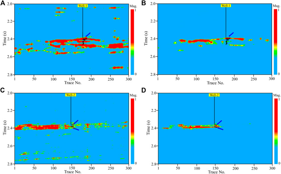
FIGURE 6. The comparison of the dispersion attribute section of P-wave and the fluid mobility. (A) and (C) are the dispersion attribute sections of P-wave. (B) and (D) are the fluid mobility sections calculated by the proposed method. The results of (A) and (B) correspond to the stacked section in Figure 5A, and the results of (C) and (D) correspond to the stacked section in Figure 5D.

To further illustrate the accuracy of the method, we choose the dispersion and fluid mobility curves at the location of the Well to compare with the log curve. Figure 7A is the seismic trace chosen from the location of Well-1. Figure 7B shows the water saturation curve, which can significantly distinguish the reservoir (outlined by the yellow shadow) with high gas saturation. Figures 7C,D show the comparison result of the dispersion curve and fluid mobility curve. Both the curves show significant anomalies in the gas-saturated reservoir. However, the dispersion curve is greatly affected by the other anomalies (indicated by black arrows) unrelated to reservoirs. The fluid mobility curve obtained by our method only shows significant anomalies in the gas-saturated zone, whereas the background interference of the other layers is very weak. Similarly, Figure 8 shows the analysis result of the curves chosen from the location of Well-2. The S_w curve in Figure 8B illustrates that there develop two sets of reservoirs with high gas saturation in the vertical direction. As shown in Figure 8C, the dispersion curve shows the strongest anomalies at the lower reservoir while the dispersion anomalies of the upper reservoir are not evident. Meanwhile, the dispersion curve is also affected by the other anomalies (indicated by the black arrows) unrelated to reservoirs. However, both reservoirs show strong anomalies in the fluid mobility curve (Figure 8D) and correlate well with the reservoir location. In addition, the anomalies of background interference are suppressed to the greatest extent. The analysis in Figure 7 and Figure 8 illustrates that the fluid mobility calculated by our method can accurately delineate the location of the reservoir and degrade the background interference of other layers unrelated to reservoirs to the most extent.

FIGURE 7

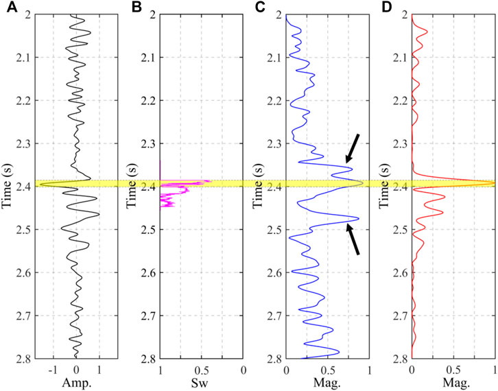
FIGURE 7. The analysis of the single trace at the location of well-1. (A) The seismic trace. (B) The log curve of water saturation. (C) The dispersion curve and (D) the fluid mobility curve correspond to the (A).

FIGURE 8

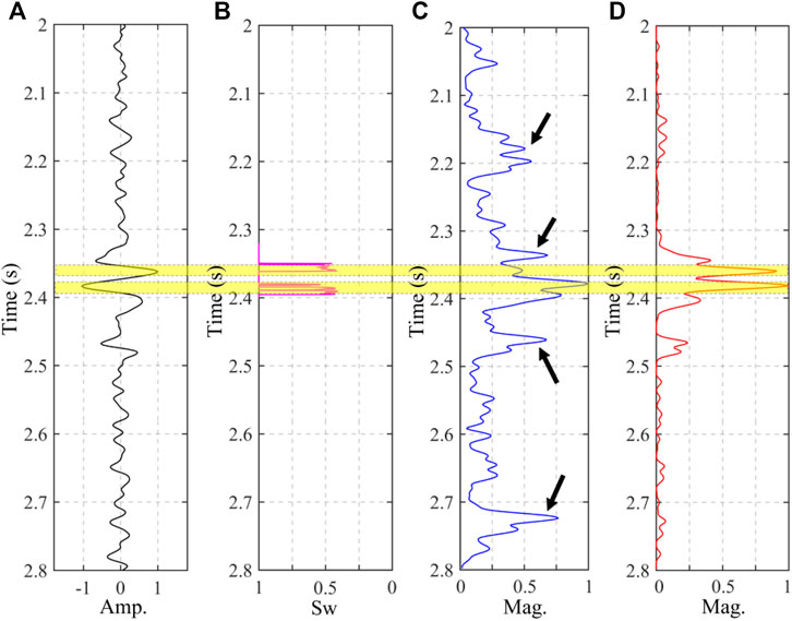
FIGURE 8. The analysis of the single trace at the location of well-2. (A) The seismic trace. (B) The log curve of water saturation. (C) The dispersion curve and (D) the fluid mobility curve correspond to the (A).

Finally, we use the proposed method to calculate the fluid mobility for 3D seismic data volume. The target interval slices extracted from the data volume are shown in Figure 9. Figure 9A is the seismic amplitude slice and Figure 9B is the fluid mobility slice corresponding to the Figure 9A. As shown in Figure 9B, both wells in the zone show strong anomalies that correlate well with the known production according to the logging interpretation results. Moreover, the fluid mobility slice clearly delineates the spatial distribution and the edge of the gas-saturated reservoirs.

FIGURE 9

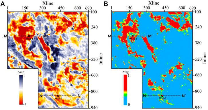
FIGURE 9. (A) Seismic slice extracted through the gas reservoir in the target interval and (B) its fluid mobility slice calculated by the proposed method. The M, M’, N and N’ donate the location of the seismic sections in the study.

Discussion and Conclusion

Based on the calculation formula of fluid mobility and frequency-dependent AVO inversion theory, a methodology for calculating frequency-dependent fluid mobility using post-stacked seismic data is proposed. In comparison with the LF-FM method, the fluid mobility calculated by the proposed method can better delineate the spatial distribution shape. Furthermore, compared with the prestack dispersion attribute inversion method (Wilson et al., 2009; Wu et al., 2012; Chen et al., 2014; Luo et al., 2020), the computation time is significantly reduced. For the seismic data corresponding to Figure 5A, it needs 41.28 s to get the results of dispersion parameters using prestack dispersion AVO inversion. However, the computation time only costs 5.92 s when obtaining the fluid mobility result. This illustrates that the proposed method is advantageous if we need to compute the large-scale seismic data volume to delineate reservoirs in a 3D area. In addition to significant computation time reductions, the fluid mobility calculated by the proposed method has a higher accuracy for reservoir characteristics compared with the dispersion attribute, which can better delineate the reservoir location. However, the prestack data contains more abundant information related to the reservoirs. If the frequency-dependent fluid mobility attribute can be extracted from the prestack seismic data, the accuracy of reservoir prediction and fluid identification will be further improved. It is worth further studying to deduce the AVO approximation related to reservoir fluid mobility from the theory of fluid-saturated porous media.

In addition, the time-frequency analysis method can directly affect the spatial resolution of the calculation result. In the proposed method, the time-frequency decomposition is conducted by the generalized S-transform proposed by Chen et al. (2009). Combining the high-precision time-frequency transform methods with the proposed method to improve the resolution and accuracy of calculation requires further investigations.

Synthetic and field data examples illustrate that the fluid mobility attribute calculated by the proposed method shows excellent imaging quality for gas-saturated reservoirs and is less affected by the anomalies unrelated to the reservoirs, which can accurately delineate the spatial distribution of hydrocarbon reservoirs. This methodology provides a new approach to extract frequency-dependent information related to the hydrocarbon reservoirs from seismic data. The calculation results can provide technical support for subsequent high-precision exploration such as fine reservoir evaluation and drilling deployment. It is noteworthy that the proposed method for calculating fluid mobility is not constrained by the well data, which also provides a new way for reservoir characterization in the case of no drilling.

Data Availability Statement

The modeling data that the findings of this study are based on are available from the corresponding author upon reasonable request. The authors do not have the legal right to release the real seismic data, and it is used for research purposes only.

Author Contributions

XL and XC contributed to the conception and design of the study. XL prepared the original draft. YD and SC prepared some Figures. YQ contributed to the data modeling. FH organized the study and modified the manuscript. All authors contributed to the article and approved the submitted version.

Funding

This work was supported by the Central Funds Guiding the Local Science and Technology Development (Grant No. 2021ZYD0037).

Conflict of Interest

Author YD is employed by No.2 Oil Production Plant, Petrochina Dagang Oilfield Company.

The remaining authors declare that the research was conducted in the absence of any commercial or financial relationships that could be construed as a potential conflict of interest.

Publisher’s Note

All claims expressed in this article are solely those of the authors and do not necessarily represent those of their affiliated organizations, or those of the publisher, the editors and the reviewers. Any product that may be evaluated in this article, or claim that may be made by its manufacturer, is not guaranteed or endorsed by the publisher.

References

Batzle, M. L., Han, D.-H., and Hofmann, R. (2006). Fluid Mobility and Frequency-dependent Seismic Velocity - Direct Measurements. Geophysics 71, N1–N9. doi:10.1190/1.2159053

CrossRef Full Text | Google Scholar

Biot, M. A. (1956b). Theory of Propagation of Elastic Waves in a Fluid‐Saturated Porous Solid. II. Higher Frequency Range. The J. Acoust. Soc. America 28, 179–191. doi:10.1121/1.1908241

CrossRef Full Text | Google Scholar

Biot, M. A. (1956a). Theory of Propagation of Elastic Waves in a Fluid‐Saturated Porous Solid. I. Low‐Frequency Range. J. Acoust. Soc. America 28, 168–178. doi:10.1121/1.1908239

CrossRef Full Text | Google Scholar

Chapman, M., Liu, E., and Li, X.-Y. (2006). The Influence of Fluid-Sensitive Dispersion and Attenuation on AVO Analysis. Geophys. J. Int. 167, 89–105. doi:10.1111/j.1365-246X.2006.02919.x

CrossRef Full Text | Google Scholar

Chapman, M., Maultzsch, S., Liu, E., and Li, X.-Y. (2003). The Effect of Fluid Saturation in an Anisotropic Multi-Scale Equant Porosity Model. J. Appl. Geophys. 54, 191–202. doi:10.1016/j.jappgeo.2003.01.003

CrossRef Full Text | Google Scholar

Chen, S., Li, X. Y., and Wu, X. (2014). Application of Frequency-dependent AVO Inversion to Hydrocarbon Detection. J. Seism. Explor. 23, 241–264.

Google Scholar

Chen, X.-H., He, Z.-H., Zhu, S.-X., Liu, W., and Zhong, W.-L. (2012). Seismic Low-Frequency-Based Calculation of Reservoir Fluid Mobility and its Applications. Appl. Geophys. 9, 326–332. doi:10.1007/s11770-012-0340-6

CrossRef Full Text | Google Scholar

Chen, X., He, Z., Gao, G., He, X., and Zou, W. (2013a). “A Fast Combined Method for Fluid Flow Related Frequency-Dependent AVO Modeling,” in 83th Annual International Meetting Expanded Abstracts. Houston, TX: SEG, 3454–3459. doi:10.1190/segam2013-0007.1

CrossRef Full Text | Google Scholar

Chen, X., He, Z., Pei, X., Zhong, W., and Yang, W. (2013b). Numerical Simulation of Frequency-dependent Seismic Response and Gas Reservoir Delineation in Turbidites: A Case Study from China. J. Appl. Geophys. 94, 22–30. doi:10.1016/j.jappgeo.2013.04.005

CrossRef Full Text | Google Scholar

Chen, X. H., He, Z. H., Huang, D. J., and Wen, X. T. (2009). Low Frequency Shadow Detection of Gas Reservoirs in Time-Frequency Domain. Chin. J. Geophys. 52, 215–221.

Google Scholar

Chen, X., Qi, Y., He, X., He, Z., and Chen, H. (2016). Phase-Shifted Based Numerical Method for Modeling Frequency-dependent Effects on Seismic Reflections. Pure Appl. Geophys. 173, 2899–2912. doi:10.1007/s00024-016-1290-3

CrossRef Full Text | Google Scholar

Dupuy, B., and Stovas, A. (2014). Influence of Frequency and Saturation on AVO Attributes for Patchy Saturated Rocks. Geophysics 79, B19–B36. doi:10.1190/geo2012-0518.1

CrossRef Full Text | Google Scholar

Goloshubin, G., Silin, D., Vingalov, V., Takkand, G., and Latfullin, M. (2008). Reservoir Permeability from Seismic Attribute Analysis. The Leading Edge 27, 376–381. doi:10.1190/1.2896629

CrossRef Full Text | Google Scholar

Gurevich, B., Makarynska, D., de Paula, O. B., and Pervukhina, M. (2010). A Simple Model for Squirt-Flow Dispersion and Attenuation in Fluid-Saturated Granular Rocks. Geophysics 75, N109–N120. doi:10.1190/1.3509782

CrossRef Full Text | Google Scholar

He, Z., Xiong, X., and Bian, L. (2008). Numerical Simulation of Seismic Low-Frequency Shadows and its Application. Appl. Geophys. 5, 301–306. doi:10.1007/s11770-008-0040-4

CrossRef Full Text | Google Scholar

Jin, H., Liu, C., Guo, Z., Zhang, Y., Niu, C., Wang, D., et al. (2021). Rock Physical Modeling and Seismic Dispersion Attribute Inversion for the Characterization of a Tight Gas Sandstone Reservoir. Front. Earth Sci. 9, 1–11. doi:10.3389/feart.2021.641651

CrossRef Full Text | Google Scholar

Kozlov, E. (2007). Seismic Signature of a Permeable, Dual-Porosity Layer. Geophysics 72, SM281–SM291. doi:10.1190/1.2763954

CrossRef Full Text | Google Scholar

Liu, J., He, Z.-L., Liu, X., Wu, H., Liu, X.-w., Huo, Z.-z., et al. (2019). Using Frequency-dependent AVO Inversion to Predict the "sweet Spots" of Shale Gas Reservoirs. Mar. Pet. Geology. 102, 283–291. doi:10.1016/j.marpetgeo.2018.12.039

CrossRef Full Text | Google Scholar

Luo, X., Chen, X., Sun, L., Zhang, J., and Jiang, W. (2020). Optimizing Schemes of Frequency-dependent Avo Inversion for Seismic Dispersion-Based High Gas-Saturation Reservoir Quantitative Delineation. J. Seism. Explor. 29, 173–199.

Google Scholar

Luo, Y., Huang, H., Yang, Y., Hao, Y., Zhang, S., and Li, Q. (2018). Integrated Prediction of deepwater Gas Reservoirs Using Bayesian Seismic Inversion and Fluid Mobility Attribute in the South China Sea. J. Nat. Gas Sci. Eng. 59, 56–66. doi:10.1016/j.jngse.2018.08.019

CrossRef Full Text | Google Scholar

Pride, S. R., Harris, J. M., Johnson, D. L., Mateeva, A., Nihel, K. T., Nowack, R. L., et al. (2003). Permeability Dependence of Seismic Amplitudes. The Leading Edge 22, 518–525. doi:10.1190/1.1587671

CrossRef Full Text | Google Scholar

Qin, X., Li, X.-y., Chen, S., and Liu, Y. (2018). The Modeling and Analysis of Frequency-dependent Characteristics in Fractured Porous media. J. Geophys. Eng. 15, 1943–1952. doi:10.1088/1742-2140/aac130

CrossRef Full Text | Google Scholar

Ren, Y., Chapman, M., Wu, X., Guo, Z., U, J., and Li, X. (2013). “Estimation of Fluid Mobility From Frequency Dependent Azimuthal AVO - A Modelling Study,” in 83th Annual International Meetting Expanded Abstracts. Houston, TX: SEG, 473–477. doi:10.1190/segam2013-1364.1

CrossRef Full Text | Google Scholar

Rubino, J. G., Velis, D. R., and Holliger, K. (2012). Permeability Effects on the Seismic Response of Gas Reservoirs. Geophys. J. Int. 189, 448–468. doi:10.1111/j.1365-246X.2011.05322.x

CrossRef Full Text | Google Scholar

Rusakov, P., Goloshubin, G., Tcimbaluk, Y., and Privalova, I. (2016). An Application of Fluid Mobility Attribute for Permeability Prognosis in the Crosswell Space with Compensation of the Reservoir Thickness Variations. Interpretation 4, T157–T165. doi:10.1190/INT-2015-0096.1

CrossRef Full Text | Google Scholar

Silin, D. B., Korneev, V. A., Goloshubin, G. M., and Patzek, T. W. (2006). Low-frequency Asymptotic Analysis of Seismic Reflection from a Fluid-Saturated Medium. Transp Porous Med. 62, 283–305. doi:10.1007/s11242-005-0881-8

CrossRef Full Text | Google Scholar

Silin, D., and Goloshubin, G. (2010). An Asymptotic Model of Seismic Reflection from a Permeable Layer. Transp Porous Med. 83, 233–256. doi:10.1007/s11242-010-9533-8

CrossRef Full Text | Google Scholar

Smith, G. C., and Gidlow, P. M. (1987). Weighted Stacking for Rock Property Estimation and Detection of Gas*. Geophys. Prospect. 35, 993–1014. doi:10.1111/j.1365-2478.1987.tb00856.x

CrossRef Full Text | Google Scholar

Wang, P., Li, J., Chen, X., Wang, K., and Wang, B. (2019). Fluid Discrimination Based on Frequency-dependent AVO Inversion with the Elastic Parameter Sensitivity Analysis. Geofluids 2019, 1–13. doi:10.1155/2019/8750127

CrossRef Full Text | Google Scholar

Wilson, A., Chapman, M., and Li, X. Y. (2009). Frequency-dependent AVO Inversion. 79th Annu. SEG Meet. Expand. Abstr.. Houston, TX: SEG 28, 341–346.

Google Scholar

Wu, X., Chapman, M., and Li, X.-Y. (2010). Estimating Seismic Dispersion from Pre-stack Data Using Frequency-Dependent AVO Inversion. 80th Annu. Int Meet. Expand. Abstr.. Denver, CO: SEG, 425–429. doi:10.1190/1.3513759

CrossRef Full Text | Google Scholar

Wu, X., Chapman, M., and Li, X.-Y. (2012). Frequency-dependent AVO Attribute: Theory and Example. First Break. Denver, CO: SEG 30, 67–72. doi:10.3997/1365-2397.2012008

CrossRef Full Text | Google Scholar

Xue, Y.-J., Cao, J.-X., Zhang, G.-L., Cheng, G.-H., and Chen, H. (2018). Application of Synchrosqueezed Wavelet Transforms to Estimate the Reservoir Fluid Mobility. Geophys. Prospecting 66, 1358–1371. doi:10.1111/1365-2478.12622

CrossRef Full Text | Google Scholar

Zhang, Y., Wen, X., Jiang, L., Liu, J., Yang, J., and Liu, S. (2020). Prediction of High-Quality Reservoirs Using the Reservoir Fluid Mobility Attribute Computed from Seismic Data. J. Pet. Sci. Eng. 190, 107007. doi:10.1016/j.petrol.2020.107007

CrossRef Full Text | Google Scholar