Grain-Size Analysis of Ancient Deep-Marine Sediments Using Laser Diffraction

Grain-size analysis of siliciclastic sedimentary rocks provides critical information for interpreting flow dynamics and depositional environments in sedimentary systems and for analysing reservoir quality of sandstone. Methods such as sieving and thin-section analysis are time consuming and unsuited for large sample numbers. Laser diffraction particle analysis is quick and reliable for analysing 100s of samples, assuming successful disaggregation. Here, we evaluate this method utilizing samples from three siliciclastic formations in Northern Italy: the Miocene Castagnola and Marnoso-Arenacea Formations, and the Cretaceous to Palaeocene Gottero Formation, which vary in degree of lithification. We focus on: 1) methods of whole-rock disaggregation; 2) methods of subsampling sediment for laser diffraction analysis; and 3) comparison of thin-section analysis with laser-diffraction particle size analysis. Using an ultrasonic bath and a SELFRAG (high voltage selective fragmentation) as disaggregation tools, this study evaluates separation of whole, undamaged grains subsequently measured by laser diffraction analysis. We show that it is possible to disaggregate ancient, well cemented rocks using an ultrasonic bath. When disaggregating samples with the SELFRAG method, grain-size measurements become less accurate and less precise with increasing sample lithification and increased presence of cement. This is likely a combination of incomplete grain disaggregation in the SELFRAG and heterogeneity within samples. Following disaggregation, we compare sub-sampling methods using a stirrer plate versus a pipette. Both produce accurate analyses, but the stirrer method is the most reliable and replicable. A comparative small subsample method, run as one whole sample with no need for subdivision into aliquots, is found to be reliable and replicable but is more susceptible to heterogeneity within field samples. When comparing laser diffraction results to grain-size volume methods estimated from thin-section analysis, thin-section sand grains are overestimated, and clay/silt grains are inaccurate. These results provide a framework for understanding potential biases introduced through various sample preparation and measurement methods.

Introduction

Grain-size analysis is ubiquitously employed by sedimentologists, geomorphologists, geographers and civil engineers working with outcrop and core datasets in clastic sedimentary systems. In detailed studies, where a description using a hand-lens is insufficient, further methods are required to build a more quantitative description of grain-size and sorting. Older methods for grain-size analysis are based on sedimentation rates for fine-grained (clay to silt) fractions and sieving for coarse-grained (silt and larger) fractions (Buller and McManus, 1972; Gee and Bauder, 1986). These methods have some drawbacks, such as they are time-consuming, very dependent on laboratory technique and operator error (Syvitski, 1991) and a large amount of material is needed (at least 10 g). These classic techniques are therefore not suitable for rapid, accurate analysis of many samples. Techniques such as thin-section analysis and laser particle-size analysis have become the norm when analysing cemented rock (Krumbein, 1935; Chayes, 1950; Greenman, 1951; Rosenfeld, et al., 1953; Friedman, 1958; Smith, 1966; Sahu, 1968; Harrell and Eriksson, 1979; Kong, et al., 2005) and unconsolidated sediment/soil (Konert and Vandenberghe, 1994; Blott, et al., 2004; Di Stefano, et al., 2010; Zihua, et al., 2009), respectively.

The time-consuming nature of thin-section point counting has been somewhat abated by newer image analysis techniques (Mazzullo and Kennedy, 1985; Francus, 1999; Persson, 1998; Van den Berg, et al., 2002; Van Den Berg, et al., 2003; Seelos and Sirocko, 2005; Fernlund, et al., 2007; Resentini, et al., 2018), but these methods can have their own technical issues, and beyond that, the time and money necessary to make thin-sections significantly limits the number of samples that can be processed. Within the last couple of decades, laser diffraction analysis has become more common, but is primarily utilized for unconsolidated sediment and soil (Konert and Vandenberghe, 1994; Sperazza, et al., 2004; Cheetham, et al., 2008; Di Stefano, et al., 2010) or in relatively young, Holocene/Pliocene-Pleistocene sedimentary rocks that are poorly lithified (Barrett and Anderson, 2000; Ito, 2008; Zihua, et al., 2009; Bralower, et al., 2010). In deepwater clastic systems, laser diffraction analysis has been effective at characterizing subtle changes in grain-size distributions in unconsolidated sediment (Stevenson et al., 2014), but the method has been under-utilized in ancient clastic systems because of challenges in disaggregating well-lithified samples (Loope, et al., 2012; Maithel, et al., 2019).

Recent studies have shown that disaggregation of lithified rocks and grain-size measurement of the sand-sized fraction through laser diffraction can be a useful tool in ancient sand-rich sedimentary systems (Maithel, et al., 2019), but the clay fraction can be altered or damaged by disaggregation methods, which commonly include crushing or chemical disaggregation. Crushing of aggregate grains (Barrett and Anderson, 2000; Jiang and Liu, 2011; Maithel, et al., 2019) can add uncertainties by fracturing or damaging grains and should therefore be avoided where possible. Chemical disaggregation has often been applied to well-lithified samples (Suczek, 1983; Triplehorn, et al., 2002; Maithel, et al., 2019). This is a useful method, but it may dissolve or abrade some minerals and can be time consuming, taking hours or days. Sodium hexametaphosphate (Na₆ [(PO₃)₆]/NaHMP) is a relatively gentle chemical method of disaggregation which is used to deflocculate clays within a sample (Sridharan, et al., 1991; Andreola, et al., 2004; Andreola, 2006) and therefore is useful as a complimentary method after other disaggregation techniques are used on the larger grains (Zihua, et al., 2009).

High-voltage selective fragmentation (SELFRAG) can be an effective tool in rock disaggregation (van der Wielen, et al., 2013). This method is most commonly used for mineral analysis in the mining industry (Andres, 2010; Wang, et al., 2011; Wang, et al., 2012; Zuo, et al., 2015), but in this study the SELFRAG method is used for siliciclastic sedimentary rocks in order to establish whether it is a reliable method for disaggregation prior to laser diffraction grain-size analysis.

Aims/Objectives

The aim of this study is to create a replicable and relatively quick method for disaggregating ancient clastic sediments and preparing them for laser diffraction grain-size analysis. This will therefore allow quicker and more accurate processing of multiple samples from the ancient rock record. Objectives are: i) to produce a reliable and repeatable workflow for disaggregating ancient mudstone and sandstone utilizing an ultrasonic bath and/or a SELFRAG machine; ii) Evaluate the reliability and potential biases associated with various subsampling methods for laser diffraction grain-size analysis; and iii) to compare the results to thin-section analysis of the same samples.

Methods

Sampling

The samples used in this study were collected from deepwater turbidites and hybrid event beds/linked debrites (Haughton, et al., 2003; Hodgson, 2009; Sumner, et al., 2009; Talling, 2013) from three basins located in north-west and central Italy with ages spanning from the Cretaceous to Miocene (Figure 1A). In total, 338 samples were collected and processed for grain-size analysis. Results from nine field samples are presented in this paper as examples for method development.

FIGURE 1

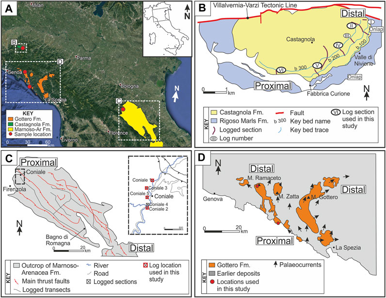
FIGURE 1. (A) Locations of three basins in Northern Italy, the Castagnola Formation, the Marnoso-Arenacea Formation and the Gottero Formation, inset map of Italy in the top right corner. (B) Outline of the Castagnola Formation outcrops (deepwater sandstone and mudstone succession) stratigraphically above the Rigoso Marls Formation, South of the Villalvernia—Varzi tectonic line (modified from Patacci et al., 2020). (C) Outline of outcrops of the Marnoso-Arenacea Formation in the Northern subbasin of the Marnoso-Arenacea foredeep, with the location of the main thrust faults through the section and logged tracts from Amy and Talling (2006). Inset map of key proximal locations in the village of Coniale (modified from Amy and Talling, 2006). (D) Location of Gottero Formation outcrops with proximal locations on the coast and distal location at Mount Ramaceto, modified from Fonnesu et al., 2018.

Castagnola Formation

The Castagnola Formation is a deep-marine unit of the Aquitanian-Burdigalian sedimentary fill of the eastern part of the Tertiary Piedmont Basin of north-west Italy (Andreoni, et al., 1981; Cavanna, et al., 1989; Di Giulio and Galbiati, 1993). The sandstone composition of the Castagnola Formation varies throughout the sections from Arkosic to Mixed to Litharenite (Figure 7 of Patacci et al., 2020). The sandstone composition of the studied interval (Beds 208, 209 and 210 sensu Southern et al., 2015) is arkosic with calcite cementation (on average Q60, F30, L10) and is interpreted to be sourced from continental basement units with limited Permian cover (Patacci, et al., 2020). Samples were taken vertically through these three beds from four logged locations (VI, V, IV and II; Southern et al., 2015; Figure 1B) in a dip to oblique section to overall palaeoflow. Bed thicknesses range from 1.5—5 m and samples were selected vertically through beds at 20 cm intervals. This formation is poorly lithified. Sandstone was easily sampled with a hammer and chisel and mudstone-rich samples were broken by hand.

In this methodological analysis, we present results from the following samples (naming convention is log—bed—sample; Figure 1B and Southern et al., 2015 for log locations and bed details):

- IV B210 S5 is from the sand-rich lower division (H1) of a hybrid event bed.

- II B209 S9 is from a dewatered/soft-sediment deformed, clast-rich lower division (H1b) of a hybrid event bed.

- V B209 S22 is from an argillaceous upper division (H5) of a hybrid event bed.

- VI 208 S2 is from sand-rich lower division (H1) of a hybrid event bed.

Marnoso- Arenacea Formation

The Miocene Marnoso-Arenacea Formation was deposited in a deepwater basin plain environment of a foreland basin (Lucchi and Valmori, 1980; Argnani and Lucchi, 2001; Amy and Talling, 2006; Muzzi Magalhaes and and Tinterri, 2010) and is now exposed in the Apennine fold-and-thrust belt within Central Italy. The samples were collected from a section that is Serravillian in age, directly above the marker Contessa megabed (Lucchi and Valmori, 1980; Amy and Talling, 2006). The sandstone is a calcite cemented quartz arenite with subordinate feldspar, biotite and lithic grains (Amy, et al., 2016), with an estimated 54% Quartz, 28% Feldspar and 18% lithic fragments (Valloni and Zuffa, 1984).

Samples were collected at 20 cm stratigraphic intervals through four beds (Bed 0, 0.4, one and two sensu Amy and Talling, 2006) from four logged locations (Coniale 1, 2, 4 and 5; locations 1, 81, 27 and 82 from Figure 9 of Amy and Talling, 2006) in a oriented perpendicular to the overall palaeoflow (Figure 1C). Bed thicknesses range from 0.3 to 1.8 m. This formation has “moderate” lithification. Sandstone samples was easily sampled with a hammer and chisel, while finer, mudstone-rich sections were more cemented and difficult to sample, with one sample uncollectable with the tools at hand.

Analysed samples come from two sections in the Coniale area—Coniale 1 (C1), which corresponds to log one of Amy and Talling (2006) and Coniale 2 (C2), which corresponds to log 80 of Amy and Talling (2006). Naming convention is Log—Bed—Sample:

- C1 B2 S1 is in the lower sand-rich division of a turbidite bed (Ta/b).

- C1 B2 S4 is in the mud-rich division of a turbidite bed (Te).

- C2 B0.4 S7 is from the argillaceous upper division (H5) of a hybrid event bed.

- C2 B1 S5B is from the argillaceous upper division (H5) of a hybrid event bed.

Gottero Formation

The Gottero deepwater turbidite system is Maastrichtian to early Palaeocene in age (Passerini and Pirini, 1964; Marroni, 1990; Marroni, et al., 2004) and was deposited onto oceanic crust in a trench basin (Abbate and Sagri, 1970; Nilsen and Abbate, 1984). The Gottero sandstone is a feldspathic wackestone, with an estimated 51% Quartz, 39% Feldspar and 10% lithic fragments (Valloni and Zuffa, 1984). Grains contain fragments of metamorphic, volcanic and sedimentary rocks (Malesani, 1966; Pandolfi, 1997) derived from the Sardo-Corso massif, where large igneous crystalline masses were exposed (Parea, 1965; Valloni and Zuffa, 1981; van de Kamp and Leake, 1995). Samples are cemented with quartz and calcite (van de Kamp and Leake, 1995). Samples were collected through three beds in a proximal area (Figure 1D) and two beds in a distal area (Figure 1D) at 50 cm intervals or at major lithological changes. Beds in the proximal area are 0.3–1.6 m thick and beds in the distal area are 1.5–2.2 m thick. This formation is well lithified with sandstone samples very difficult to take with a hammer and chisel. Wider spacing in sampling was necessary due to the difficulty in removing samples and time constraints in the field.

From the distal area, Mount Ramaceto:

- GOT A B13 S3- Location ‘A’ is in the vicinity of Log F (Fonnesu et al., 2018), B13 is Bed 13 of (Fonnesu et al., 2016; Fonnesu et al., 2018), sample 3 is from a mud clast-rich section of the lower sand-rich division of a hybrid event bed (H1).

Nomenclature for Samples

The samples collected in the field were subsampled in various ways and using several methods. For clarity, we describe sample terminology for field samples, large and small subsamples, and aliquots below.

Field Samples

These are samples taken directly from the beds in the field at 20 cm intervals in the Castagnola and Marnoso-Arenacea Formations and at 50 cm intervals in the Gottero Formation. Due to the debritic nature of the deposits, some heterogeneity within field samples was unavoidable. Field samples weighed between 50 and 1,000 g.

Large or Small Subsamples

Subsamples are taken directly from field samples. A small (0.5–5 g) or large (5–10 g) piece is gently hammered from the field sample and then disaggregated for grain size analysis. Effort is made so that the piece chosen looks representative of the whole sample. Small subsamples (designated ‘S’ in Supplementary Table S1) can be directly introduced into a laser particle size analyser (LPSA) in one batch without the need for further subdivision (see obscuration limitations below for explanation on sample size). Large subsamples (designated ‘L’ in Supplementary Table S1) are over the obscuration limit and must be further split into aliquots before processing with the LPSA.

Aliquots

An aliquot is a subdivision of the larger subsamples that is sufficiently small to be introduced directly into the LPSA. These are sampled using the pipette or stirrer method (outlined below) for wet samples disaggregated with the ultrasonic bath method, or the riffle splitter for dry samples disaggregated with the SELFRAG method. Aliquots are placed directly into the laser diffraction grain-size analyser for measurement.

Equipment and Techniques Used

Samples were taken from the formations described above and disaggregated. The full method for disaggregation can be seen in Figure 2. Equipment used can be seen in Figure 3.

FIGURE 2

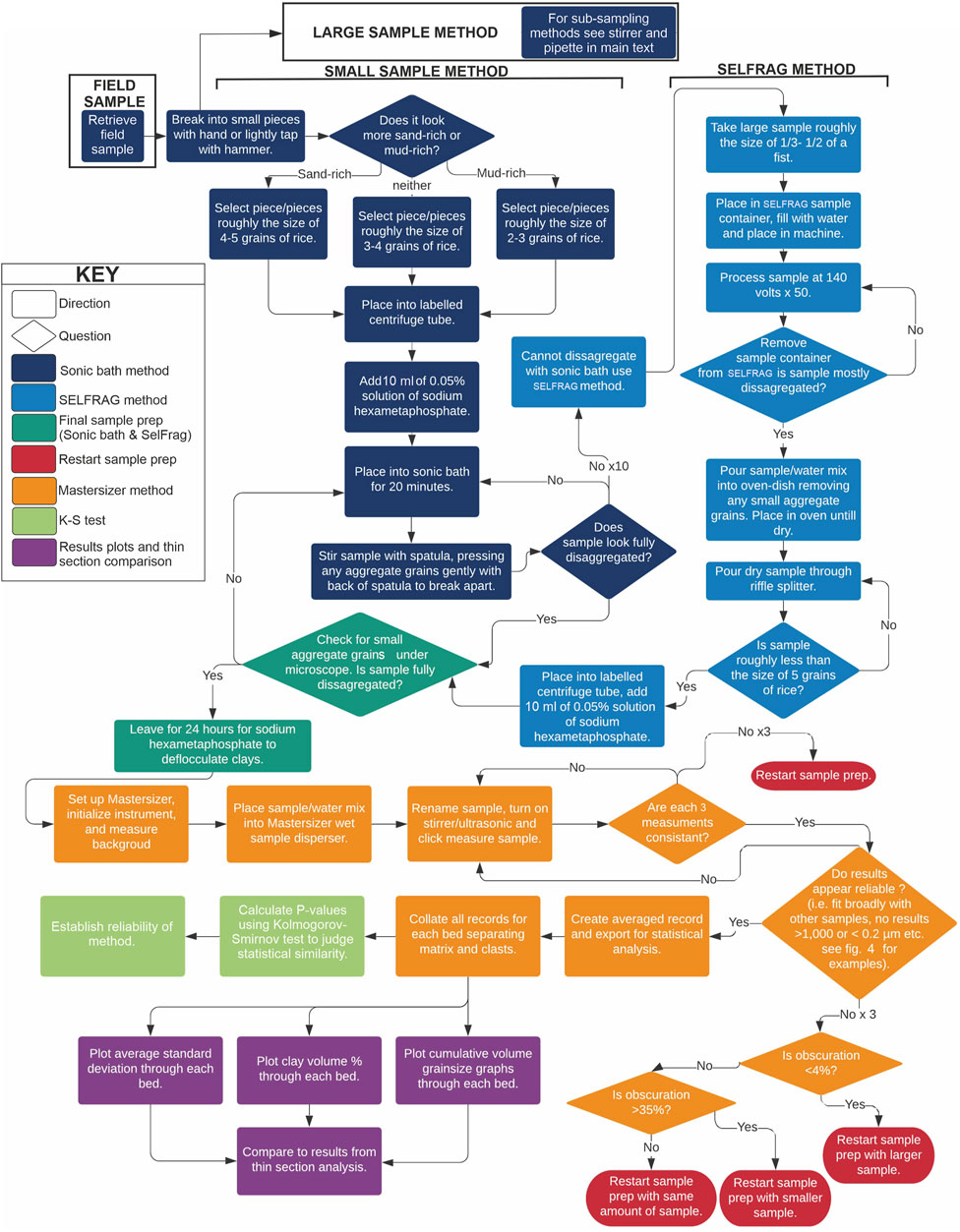
FIGURE 2. Flow chart depicting entire workflow of study, including sample disaggregation methods, grain-size analysis and data processing. Each method is further explained in the text.

FIGURE 3

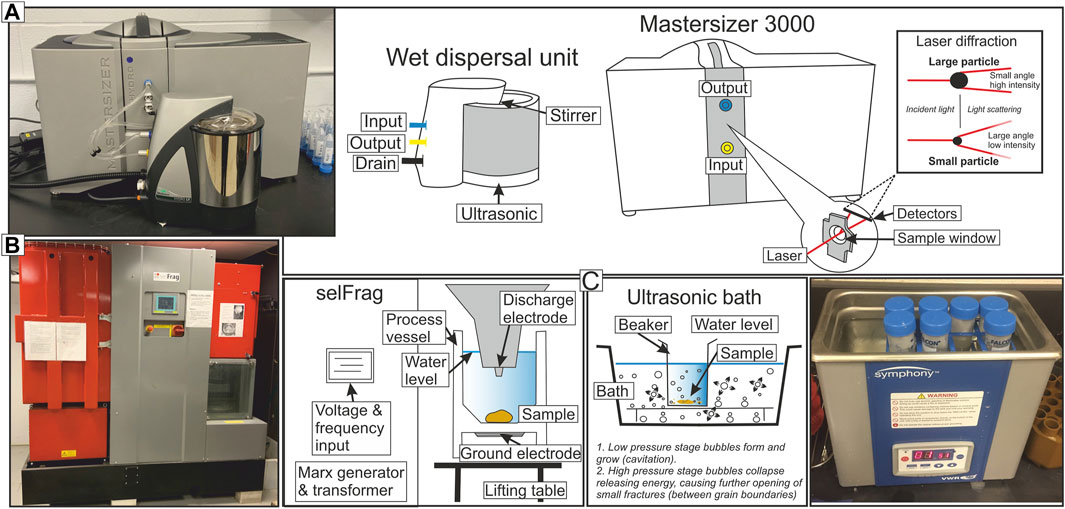
FIGURE 3. Key equipment used in this study (A) Mastersizer 3000 laser diffraction unit with wet dispersal system. (B) SELFRAG selective fragmentation machine and (C) ultrasonic bath. For use of equipment see methods flow chart in Figure 2.

Mechanical Disaggregation

Two mechanical disaggregation methods were used in this study: an ultrasonic bath and a SELFRAG machine (Figure 2).

Ultrasonic Bath

Ultrasonic baths (Figures 2, 3) use ultrasonic vibrations to break aggregate sediment apart along grain boundaries. Ultrasonic sound waves radiate through the water bath causing alternating higher and lower pressures (Figure 3C). During the low-pressure stage, microscopic bubbles form and grow, increasing cracks along grain boundaries until they eventually break apart. This has been used as a rapid and efficient sediment disaggregation method for many decades (Edwards and Bremner, 1967; Walker and Hutka, 1973; Rendigs and Commeau, 1987). There is very low risk of quartz grains being abraded and minor risk for feldspar and mica grains (Hayton, et al., 2001) and, overall, this is considered a gentle method of disaggregation with low risk of breaking sediments beyond grain-boundaries. This method is therefore used as the primary tool for disaggregation and only when unsuccessful should the SELFRAG be used. The steps for disaggregation in the ultrasonic bath method can be seen in the dark blue boxes in Figure 2. Samples took from 10 min to 1 h to be disaggregated in total. Despite this method being relatively mild, there is still the possibility that grains are broken down beyond natural grain boundaries and therefore made artificially ‘finer’ if it is overused (discussed further in “Sensitivity Test”below).

SELFRAG

A SELFRAG is a high-voltage-pulse fragmentation machine (Figures 2, 3B). This instrument can generate 90–200 kV with the number of pulses set by the user and is used on samples up to ∼1 kg. The sample is placed in a vessel and energy is discharged by electrodes with water used as a conductor. User-controlled settings are: number of pulses; discharge voltage (90–200 kV), i.e., energy per pulse; electrode gap (10–40 mm); and frequency of discharge (1–5 Hz). It works most efficiently on coarser grain-sizes (van der Wielen, et al., 2013) and was therefore used on sand-rich samples in this study. This method of disaggregation has traditionally been used on ore minerals (Wang, et al., 2011; van der Wielen, et al., 2013) and for fossil preparation (Saini-Eidukat and Weiblen, 1996). In this study we started with a lower number of pulses (e.g., 20–50) and discharge voltage (100–140 kV) and repeated as necessary to disaggregate.

Chemical Disaggregation

Sodium Hexametaphospate

Sodium hexametaphosphate (NaHMP) was added to samples after disaggregation in the ultrasonic bath or in the SELFRAG (Figure 2). This chemical is commonly used as a dispersant, not only in grain-size separation (Maithel, et al., 2019; Sperazza, et al., 2004) but in pigmenting and dyeing operations, in oil well drilling muds, and as a water softener (van Olphen, 1977; Andreola, 2006). The NaHMP solution separates clay particles, preventing them from bonding together to form ‘flocs’ through forming soluble undissociated complexes with many cations which prevents the flocculation effects (Wintermyer and Kinter, 1955). In this study we use a solution of 0.5% NaHMP in water, within the range of 0.025–0.06 g per 100 cc (Chilingar, 1952), with roughly 20 ml added to each sample. Samples are left in the NaHMP solution for 24 h before analysis.

Laser Diffraction Analysis

In this study, grain-size analysis was conducted using the Malvern Panalytical Mastersizer 3000 particle size analyser (Figures 2,3). Laser-diffraction size analysis is based on the principle that particles of a given size diffract light through a given angle, with the angle increasing as particle size decreases. The Mastersizer 3000 uses two different light sources to analyse the entire granulometric range light sources to analyse the entire granulometric range. In particular, there is a red laser with Ne-He source producing a radiation with 632.8 nm of wavelength and a blue laser emitted by a LED source with a characteristic wavelength of 470 nm. These light sources pass through a sample cell containing an upward moving suspension and the diffracted light is focused onto detectors (Figure 3A). The grain-size distribution is calculated from the light intensity reaching the array of detectors. The Mastersizer 3000 uses the full Mie theory to calculate grain-size, which completely solves the equations for interaction of light with matter. Mie theory requires the knowledge of the: Refractive Index (RI) of the grains—this value relates to the speed of light within the material, which in turn allows the degree of refraction (light bending) to be predicted when light passes from one medium to another—and the Absorption Index (AI)—a number that describes the amount of absorption that takes place as the light enters the particle. For this study the value of quartz was used with a RI of 1.54 and AI of 0.01. The size distribution is measured while the suspension is continuously pumped around, which ensures random orientation of most particles relative to the laser beam so that the equivalent spherical cross-sectional diameter is measured. The Mastersizer 3000 measures particles in the range of 10 nm–3,500 μm. This study used a wet-dispersion unit, which circulates the mixture of water and sample through the glass cell. Mie theory also assumes that the particle is spherical, therefore the grain-size results correspond to the equivalent diameter of the sphere of a grain. This means that the same grain-size will be given if two particles have the same volume but vary significantly in sphericity and roundness, allowing for more accurate comparison of grain size within and between samples. This also does not compare directly to sieving because sieving compares the b-axis of grains. The Mastersizer 3000 was set to measure each aliquot three times whilst it circulates through the glass cell, which is standard procedure to ensure that repeated measurements of the same aliquot are consistent. If these three measurements are consistent with each other, their average is used for analysis. Reasons for inconsistency could be flocculation of clays or dissolution of material during measurement. Dissolution is not relevant here because the sediment is stable, and to prevent clay flocculation during measurement an internal ultrasonic instrument was turned on during measurements. Deionized water was used for sample processing. Although the Mastersizer 3000 is used in this study, our results are broadly applicable to other brands of LPSA instruments.

Results and Method Development

The ideal grain-size analysis method is one that provides the ability to analyse several hundred samples within a reasonable timeframe, while remaining as accurate as possible. In order to establish the ideal sample preparation and measuring procedure, several different methods of sample preparation are compared. The steps investigated here focus on 1) disaggregation of lithified samples, and 2) subsampling of disaggregated sediment for laser particle size analysis. Disaggregation methods include an ultrasonic bath or high voltage electrical discharges (SELFRAG). Presumably, large samples (∼5–10 g when dry) would provide the most representative grain size distributions that span the full range of grain sizes within a given field sample, however, large subsamples typically exceed the obscuration limit (the level at which the lasers can no longer shine clearly through the sample and water mixture) of laser particle-size analysers. Division into aliquots is therefore necessary prior to running samples through the LPSA. Aliquot methods compared below include subdividing lithified samples prior to disaggregation or subdividing wet samples after disaggregation using either a) the stirrer method, or b) the pipette method, described below. A sub-sampling method for dry samples using the SELFRAG method is discussed later.

In order to compare results between various methods, and whether differences between methods is comparable to the natural variability within the samples themselves, we use the two-sample Kolmogorov-Smirnov test (KS test; Chakravarti et al., 1967) to test whether samples are statistically likely to come from the same distribution. In the KS test, the null hypothesis is that both samples come from a population with the same distribution. A high p-value therefore suggests that two distributions could be generated from the same population and a low p-value suggests the distributions are significantly different from each other. The typical significance threshold for p-values is taken as 0.05, however as illustrated by Supplementary Table S2 the p-values for all samples compared to other samples are quite high (rarely <0.1). This is likely because we are comparing samples with extremely similar distributions to one another, so statistically they are all similar. However, we can qualitatively take the p-values as an indication of how similar the distributions are to one another, with the understanding that small changes in p-value are not particularly meaningful but samples with very low p-values (e.g., p < 0.3) are likely less similar than those with very high p-values (e.g., p > 0.9).

Obscuration Limits

The suggested obscuration limits for the Mastersizer 3000 are roughly between 8 and 24% (Figure 4). The obscuration of the sample depends on the number of grains in the sample. Finer-grained samples therefore provide a higher obscuration for a given sample weight. During the measurements of this study, results were reliable with lower (3–8%) obscuration, especially with mud dominated samples, as well as with a much higher obscuration (up to 45%). Blott et al. (2004) also found that reproduceable results can be obtained with lower than recommended obscuration values. An obvious change within the grain size distribution was observed if obscuration values were too high (Figure 4), with results showing an additional smaller peak in grain sizes <0.1 µm, which is considered unreasonably small for these samples because it is not recorded in any reliable measurements. For samples with fewer grains or finer grain-sizes, increasing the measurement time for each sample may help to improve measurement accuracy, however for this study the standard measurement time of 10 s was kept throughout for consistency.

FIGURE 4

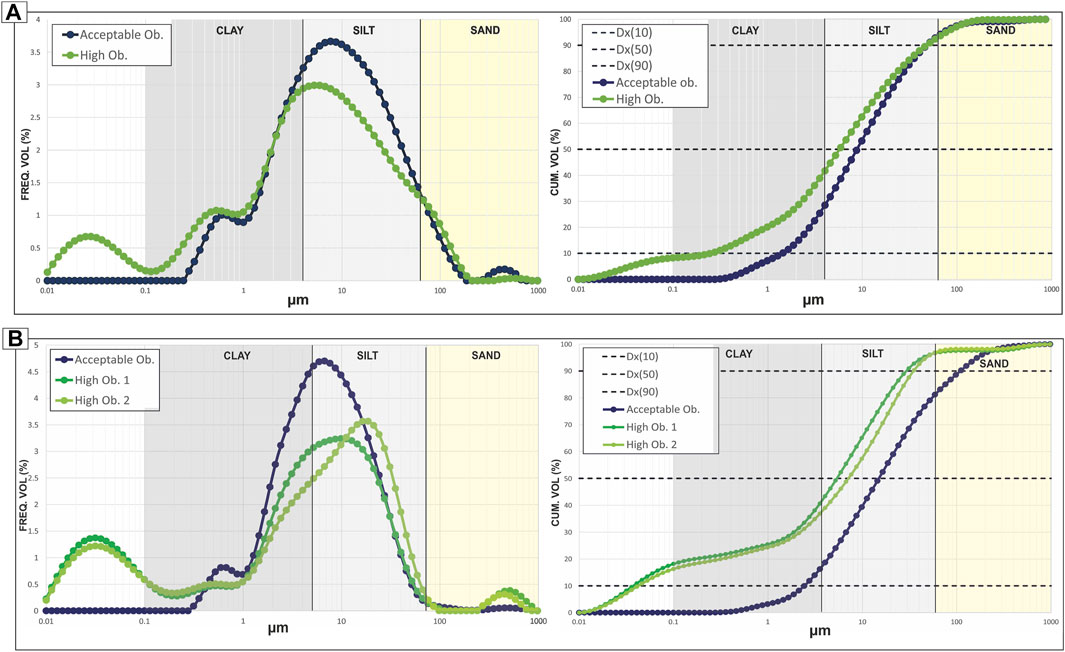
FIGURE 4. Volume frequency and cumulative frequency graphs showing two versions of the same subsample: the green with too much material added to the Mastersizer, resulting in obscuration that is above reliable measurement, and the blue showing a sample that is within obscuration limits. Data are from the Marnoso- Arenacea Formation. (A) Location Coniale 1, Bed 2 (Amy and Talling, 2006), Sample 4, interpreted as a turbidite. The acceptable obscuration in blue is 20.61%, the high obscuration in green is 26.46%. (B) Location Coniale 2, Bed 0.4 (Amy and Talling, 2006), Sample 7, interpreted as a hybrid event bed. The acceptable obscuration in blue is 19.74%, the high obscuration examples are 44.21 and 44.66%. For details Supplementary Table S1.

Sensitivity Test

In order to understand the efficacy of the ultrasonic bath in disaggregating sediments, a time trial was undertaken by measuring the grain size of the same sample after increasing intervals of time in the ultrasonic bath (Figure 5). This was also important to assess whether the ultrasonic bath was significantly breaking down grains beyond grain boundaries if left in the ultrasonic bath for a longer time period than necessary for disaggregation.

FIGURE 5

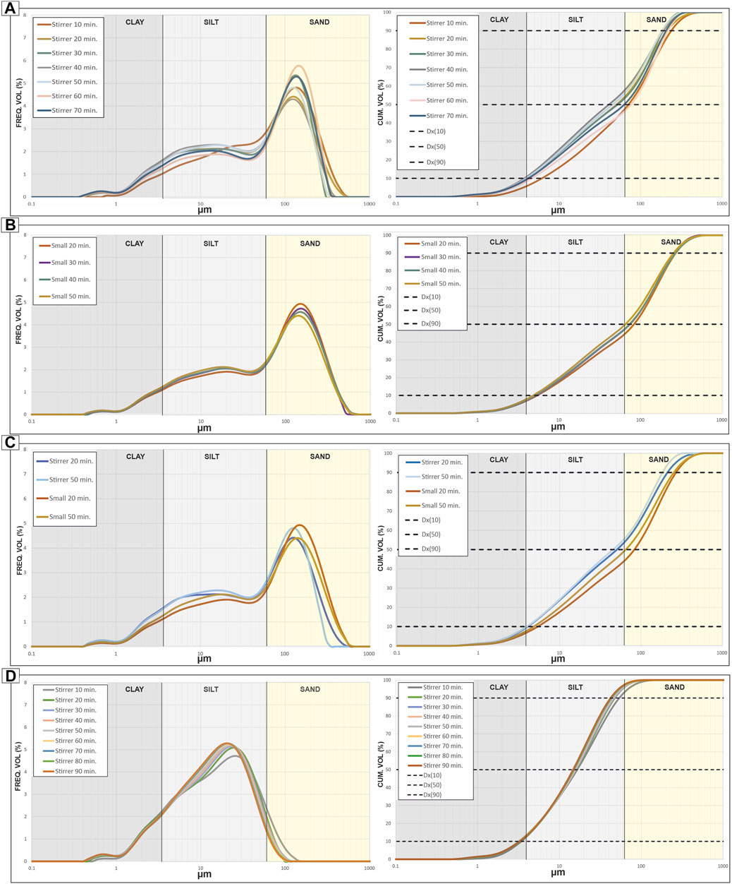
FIGURE 5. Volume frequency and cumulative frequency graphs showing timing tests for sub-samples and aliquots processed using the ultrasonic bath method. Supplementary Table S1 for full data results. (A) Field sample II B 209 S9, Large Subsample A- aliquots extracted using the stirrer method every 10 min to establish how the result changes with more time disaggregating in the ultrasonic bath. (B) Field sample II B209 S9, Subsample B,C,D,E - Small subsamples, sample tested every 10 min from 20 min to establish how result changes with more time in the ultrasonic bath disaggregating. (C) Comparison of results from (A,B) to demonstrate similarities and differences. (D) Field sample V B209 S22, Large Subample - aliquots extracted using the stirrer method, testing one sample every 10 min to establish how the result changes with more time disaggregating in the ultrasonic bath.

This trial was undertaken with two field samples (Figure 5): II B 209 S9 (Figures 5A–C), a sand-rich sample from the Castagnola Formation; and V B209 S22 (Figure 5D), a more silt-rich sample from the Castagnola Formation. Both samples were calcite cemented. For each of these field samples, a large subsample was put into a beaker with 50 ml of NaHMP solution and placed into the ultrasonic bath. Every 10 min, an aliquot was taken from the beaker and placed into the LPSA for analysis, allowing for comparison of how the grain-size distribution changed with increasing time in the ultrasonic bath. The grain-size curves initially get slightly finer through time, which we interpret as a record of larger grains disaggregating with more time in the ultrasonic bath. Eventually, around 70 min for V B209 S9 and 40 min for II B209 S9, the curves maintain similarity despite additional time in the ultrasonic bath, indicating that the samples are fully disaggregated and the distribution is remaining stable with any additional time in the ultrasonic bath. Moreover, after 20 min for V B209 S9 and 10 min for II B209 S9, the minimum grain size is stable, indicating that clay particles aren’t further broken down by further time in the ultrasonic bath and therefore no micro-fragmentation is occurring.

For Field sample II B209 S9, an additional timing test was conducted by taking 4 small subsamples (B—D in Supplementary Table S1) and each small subsample was given 20, 30, 40, and 50 min in the ultrasonic bath, respectively, and placed directly into the LPSA for analysis. This removed any potential bias tied to repeated aliquot sampling but increased potential uncertainty about whether changes in grain size were due to natural sample variability or degree of disaggregation. Overall, very little difference can be seen between the results of these subsamples (Supplementary Table S1; Figure 5B), showing that after 20 min in the ultrasonic bath the sample is well disaggregated. When the data is examined in detail (Supplementary Table S1) some evidence of further disaggregation can be noted; The d₅₀ decreases through time from 83 to 65 μm. This change in average appears to be mostly due to a decrease in the larger grains (d₉₀) change from 271 to 255 μm) and to a lesser extent by a slight increase in fines (d₁₀) changes from 5.38–4.8 μm, and increase in clay % from 7.03–8.01%). Despite this overall increase in clay and silt the minimum grain size is stable after 20 min for all samples, indicating that micro-fragmentation and breakdown along grain boundaries is not occurring.

Both sets of tests (A–C and B–D) indicate that the ultrasonic bath effectively disaggregates lithified siliciclastic rocks. Furthermore, there is no apparent concern in “over-sonicating” samples and damaging grains and the length of time needed to fully disaggregate samples will vary based on sample size, lithology, degree of cementation and modal composition. However, care should be taken with biogenic sediments because they may be at greater risk of ‘over-sonication’.

Aliquot Methods for Large Subsamples

Large subsamples weighing ∼ 5–10 g were used in order to get a representative grain size distribution for measurement. These large subsamples were placed into 50 ml centrifuge tubes with 20 ml of NaHMP solution, disaggregated with the ultrasonic bath method (Figure 2), and left for 24 h. These subsamples were too large to be processed in one pass with the Mastersizer 3000 because they would increase the obscuration beyond measurable levels (see above). Two aliquot sampling methods were therefore tested for wet dispersions and the average of all measured aliquots for a given large subsample were compared to one another in order to establish the reliability of each method.

The two aliquot sampling methods used were the stirrer method and the pipette method, outlined below.

Aliquot Sampling Method

The challenge of extracting representative aliquots from samples is not trivial, and a consistent methodology does not exist within the sedimentology community. Two common aliquot sampling methods are evaluated here: the pipette method, in which a pipette is used to agitate and then extract material from a centrifuge tube, and the stirrer method, in which the samples are placed in a beaker and a magnetic stirrer creates a suspension from which aliquots are extracted. These methods are explained in more detail below. In order to validate both the pipette and stirrer methods, two different forms of each method were evaluated using field sample V B209 S22 from the Castagnola Formation (Figure 6). This sample was collected from an argillaceous section at the top of a hybrid event bed (H5 of Haughton et al., 2009). Results are documented in Supplementary Table S1; Figures 6, 7. Three large subsamples (A, B, and C) were used for method comparison (Figure 7).

FIGURE 6

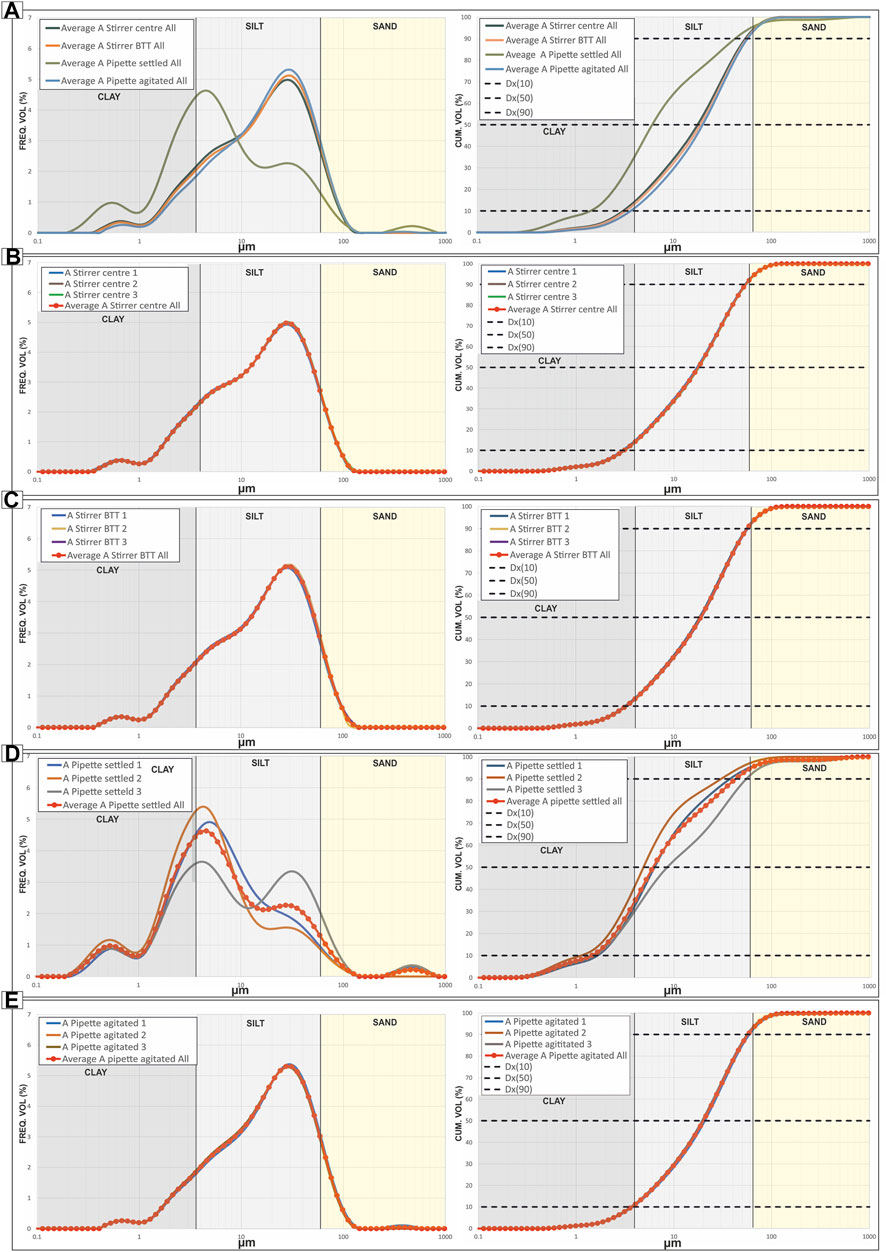
FIGURE 6. Volume frequency and cumulative frequency of aliquots for mud-rich field sample V B209 S22 using various trial methods. See text for full details. (A) Average results for all trial methods for comparison. (B) Individual results and average for the ‘Stirrer centre’ method. (C) individual results and average for “Stirrer base to top” method. (D) Individual results and average for ‘Pipette settled’ method. (E) Individual results and average for ‘Pipette agitated method’. For full data Supplementary Table S1, for corresponding p-values Supplementary Table S2.

FIGURE 7

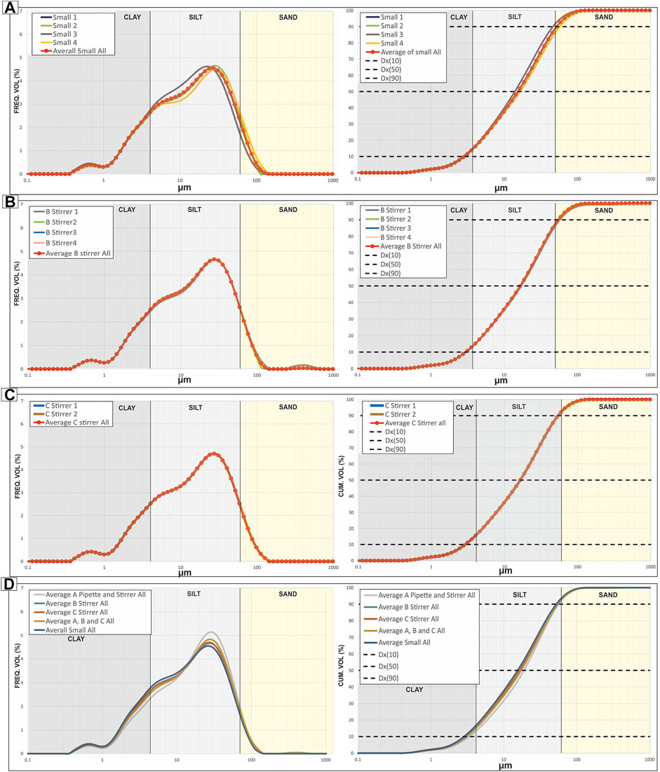
FIGURE 7. Volume frequency and cumulative frequency of aliquots for mud-rich field sample V B209 S22. These are further tests using the stirrer method and small samples to compare to subsample A results in Figure 6. (A) Small sub-samples D, E, F, G and average small sample result. (B) Sub-sample B, Stirrer aliquots 1-4 and average of aliquots. (C) Sub-sample C, Stirrer aliquots 1 and 2, and average of both aliquots (D) Averages of subsamples A, B and C, compared to an average of all of these sub-samples and an average of the small samples. For detailed results Supplementary Table S1, for p-values Supplementary Table S2.

Trial 1: Stirrer “Centre”

Subsample A was placed in a beaker with a NaHMP solution and mixed with a magnetic stir plate. The rotation of the stirrer was increased until all grains appeared to be in suspension. A 7 ml pipette with a 3 mm opening was used to extract an aliquot, approximately halfway up the sediment/water mixture and halfway between the centre and the outer edge of the beaker. Three aliquots were measured for comparison.

Results (Supplementary Table S1; Figure 6B): All recorded parameters for aliquots A Stirrer Centre 1, two and 3 are very similar. Calculated p values between the three aliquots (Supplementary Table S2) give values of 0.9999–1.0000 (at 4 decimal places), showing this method to be highly replicable.

Trial 2: Stirrer “Base to Top”

Stirring plates were set up as above, with the remaining subsample A prepared in a beaker and the rotation of the stirrer increased until all grains appeared to be in suspension. A 7 ml pipette with a 3 mm opening was then used to extract an aliquot by placing it halfway between the centre and outer edge of the beaker and sampling while moving it upwards from the base to the top of the beaker.

Results (Supplementary Table S1; Figure 6C): All recorded parameters for aliquots “A stirrer base to top” 1, 2 ,and 3 are very similar. Calculated p values (Supplementary Table S2) give values of 0.9999–1.0000. This shows this method to be highly replicable. When comparing between the “centre” and ‘base to top’ methods, p values are between 0.9956 and 1.0000, with a p value between the averages of each method of 1.0000. Therefore, little difference can be noted between these two methods for aliquot sampling, and both are replicable and representative of the subsample. This also suggests that potential grain-size stratification within the suspension was not significant.

Trial 3: Pipette “Settled”

Grains were left to fully settle to the base of the of the beaker, without any stirring. A 7 ml pipette with a 3 mm opening was inserted into the base of the mixture and whilst collecting the sample slowly moved upwards until the pipette was out of the sediment/water mixture.

Results (Supplementary Table S1; Figure 6D): Results from this method (‘A Pipette settled’ 1, 2 and 3, Supplementary Table S1; Figure 6D) were highly variable. The d₅₀ results were considerably lower when compared to both stirrer methods, with the clay content up to 28% higher than in the stirrer method. p values for comparisons between samples (Supplementary Table S2) are 0.2713–0.4938. This is still above the 0.05 range suggesting that these results are not statistically significantly different, but is less so than the other trialled methods. Therefore, this method is considered less reliable and replicable.

Trial 4: Pipette “Agitated”

For this trial, the remainder of subsample A was placed into a 50 ml centrifuge tube. A 7 ml pipette with a 3 mm opening was inserted into the mixture and pumped vigorously and continuously until all sediment was in suspension. An aliquot was then quickly taken by moving the pipette from the base of the centrifuge tube upwards through the mixture while sampling.

Results (Supplementary Table S1; Figure 6E): All parameters from aliquots ‘A pipette agitated’ 1, two and 3 are very similar. Calculated p values (Supplementary Table S2) between aliquots are 0.7695–1.0000. So, although this method is not as replicable as either stirrer method, it is still sufficiently replicable. When compared to the pipette settled method, p-values are 0.0219–0.1317 ranging below the 0.05 limit of statistical significance, again indicating that the Pipette settled method is less reliable.

Outcomes From Aliquot Trial Methods

Overall, the “centre” method for the stirrer and the ‘agitated’ method for the pipette are the most replicable methods for the stirrer and pipette, respectively (Figure 6A). These are therefore the methods used when “pipette” and “stirrer” methods are referred to hereafter. Because the stirrer method was the most replicable, additional subsamples (B & C) were used to re-test this method for comparison and to further interrogate its reliability.

Additional Stirrer Samples

Subsamples B and C (Supplementary Table S1) were taken from field sample V B209 S22 for further testing using the stirrer (centre) method (Table 1; Figures 7B–D).

Comparisons of aliquot results between subsamples A, B, and C show very little difference in d₅₀ or any other measured parameters (Supplementary Table S1). An anomaly is seen in the Average Standard Deviation (ASD) of B stirrer 1, which may be due to an anomalously large grain incorporated into this first pipette aliquot, but it does not seem to have significantly altered the d₉₀ (57.5 μm compared to average 54.9 μm values) or clay and silt percentages (92.00 compared to 93.12%). This is further distinguished by the p-values in B Stirrer one compared to all other B aliquots, which range from 0.3722–0.4938, whereas comparisons between B aliquots 2, 3 and 4 provide p-values of 1.000 (Supplementary Table S2). This indicates that averages of multiple aliquots are important to avoid any small anomalous results likely due to picking up one or two large grains.

p-values comparing “A stirrer (centre)ˮ average and “C stirrer (centre)ˮ average are 0.9999 (Supplementary Table S2). When A Stirrer and C Stirrer are compared to the B Stirrer average values the p-value is from 0.4938 to 0.6307 (Supplementary Table S2), due to the issue with the 1st aliquot in B. Overall, this stirrer method is still judged to be reliable, but care should be taken and multiple aliquots should be used and averaged to reduce risk of anomalous grains skewing results.

Small Subsample Comparison

Small Subsample Method

When evaluating aliquot sampling methods, it is important to understand natural variability within samples in order to ensure that changes are due to sampling methods and not real variability between subsamples. As discussed above, large subsamples (roughly 5–10 g) were used initially to get a representative sample that might account for slight heterogeneity within samples. Next, we investigate measurement differences between disaggregating smaller subsamples (0.2–2 g) that could be run in one batch and do not require aliquot subsampling, therefore speeding up the measurement process and potentially reducing bias introduced during the extraction of aliquots. Small subsamples ranging from 0.2 to 2.0 g were taken from field samples, with sandier samples on the large end of that range and muddier samples on the small end because mud and silt have a greater effect on obscuration and therefore require less material for measurement (Figure 2). These samples were placed in a small centrifuge tube (15 ml) along with 10 ml of NaHMP solution. The centrifuge tubes were placed in the ultrasonic bath until the samples were fully disaggregated (Figure 2). Disaggregation was determined by eye and by inspection under a microscope. The samples were then left for 24 h to ensure clays were deflocculated. Results for this method were compared to the average of subsamples for the “large subsample” methods above in order to compare natural variability between samples in the absence of any potential biases introduced through aliquot subsampling.

Small Subsample Results

Four small subsamples were taken from the same field sample used in previous trials, V B209 S22, designated D, E, F and G (Table 1; Figures 7A,D). These four small subsamples showed little variation from each other in d₅₀ (varying from 16.2 to 17.1 μm) or the clay percentage which varied from 15.48 to 16.48% (Supplementary Table S1). KS test comparisons between the small samples provided p-values ranging from 0.9956 to 1.000 (Supplementary Table S2).

The small samples have very similar d₅₀ values to the stirrer results from subsamples A, B and C. KS test comparisons between small subsamples (D–G) and stirrer samples A and C provide p-values greater than 0.9956. When compared to stirrer sample B, the p-values range from 0.2713 to 0.6307, again due to the issues with the first aliquot from the B sample. Overall, this indicates that the small subsample method is as reliable as the large subsample method, provided that the field samples are relatively homogenous. It also does not risk the inaccuracies incurred in the aliquot sampling for the stirrer method (i.e. B Stirrer 1).

Applicability to Sand-Rich Samples

Having validated the best methods for aliquot subsampling and compared these to the small sub-sample method, we now explore the utility of each method with a more sand-rich sample, which may be more susceptible to aliquot biases due to the difficulty in suspending coarser grains. Small and large subsamples were taken from the field sample II B209 S9 (Figure 8; Supplementary Table S1), which is from a dewatered, clast-rich lower division (H1b) of a hybrid event bed (Southern et al., 2015).

FIGURE 8

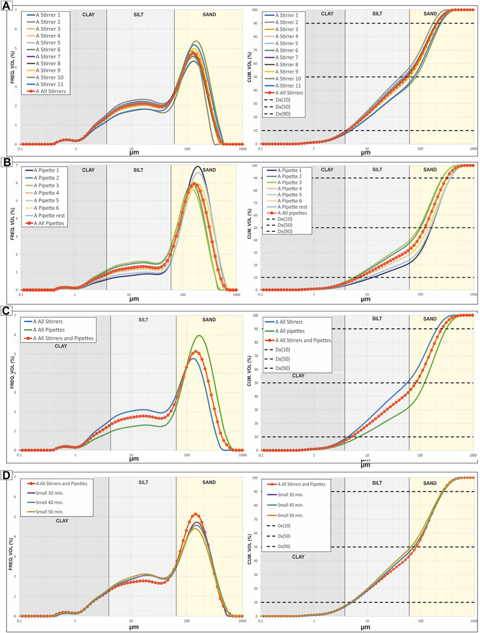
FIGURE 8. Volume frequency and cumulative frequency graphs showing aliquots for sand-rich field sample II B209 S 9, Sub-sample A, showing aliquots from the establish Pipette and Stirrer methods. (A) Stirrer aliquots 1–11 and average of all stirrer aliquots. (B) Pipette aliquots 1–7 and average of all pipette aliquots. (C) Comparison of stirrer and pipette averages and averages for all sub-sample A aliquots. (D) Average of all subsample A stirrers and pipettes compared to 3 small samples (taken from the time test in Figure 5). For detailed results Supplementary Table S1, for p-values Supplementary Table S2.

Three small samples were analysed to provide context for the natural variability within the field sample and to provide a baseline for comparing potential biases introduced with the stirrer and pipette aliquot methods. The small subsamples are overall consistent with one another (Supplementary Table S1; Figure 8D), with p-values ranging from 0.8887 to 0.9998 (Supplementary Table S2) and allow for comparison between pipette and stirrer aliquot methods extracted from a large sub-sample.

From a large subsample (subsample A), 11 aliquots were extracted using the stirrer method (Figure 8A) and seven aliquots using the pipette method (Figure 8B). Overall, the stirrer method slightly underestimates the grain size and the pipette method slightly overestimates the grain size (Figure 8C) when compared to the small samples, which we take here as a representative ‘true’ distribution of the field sample. A general increase in d₅₀ can be noted from the stirrer method aliquots 1–11, ranging from 42.7 to 75.6 μm, however these values are still much lower than the average d₅₀ value of 121 μm from the pipette method aliquots (Supplementary Table S1). The increasing trend in d₅₀ values with continued aliquot sampling is likely due to the tendency for this method to preferentially select finer grains that are more easily-suspended, meaning that continued sampling results in distributions becoming progressively coarser. However, this trend is subtle compared to the differences between the pipette and stirrer methods and the averages of all stirrer and pipette aliquots highlight the tendency for the stirrer method to preferentially select clay and silt while the pipette method preferentially selects sand-sized particles.

The stirrer method is slightly more replicable than the pipette method (Figures 8A–C), however both methods appear to be internally consistent; Grain-size distributions of aliquots sampled from sand-rich samples with the same method—either pipette or stirrer—come with their own biases. Pipette method aliquots are slightly coarser than the average of the whole sample and stirrer method aliquots are slightly finer (Figure 8C). Each method is potentially sufficient depending on whether the focus of the analysis is on fine- or coarse-grained constituents and results from different methods should be compared with caution.

p-values (Supplementary Table S2; Supplementary Material S1) are generally lower for the sand-rich sample (II B209 S9), particularly when compared to the average of all samples. However, many of the stirrer aliquots had high p-values (p > 0.6), particularly those that were sampled in close succession (Supplementary Table S2). The pipette aliquot comparisons show lower p-values, with most aliquot comparisons showing p < 0.2 and many with p < 0.05 (Supplementary Table S2).

A Note on Sample Heterogeneity

To further validate the comparisons between the stirrer, pipette and small subsample methods, analysis was undertaken using a mud-rich sample from the more lithified Marnoso-Arenacea Formation. Field sample C2 B0.4 S7 was taken from the upper mud-rich H5 division (Haughton et al., 2009) of a hybrid event bed. Importantly, this interval is also affected by bioturbation, with sand-filled burrows infilled during emplacement of the bed above. Burrows themselves were not sampled but some contamination was possible. From this field sample, two large subsamples were taken (A and B) and were analysed using both the stirrer and pipette aliquot methods, and 5 small subsamples were taken (C—G) in order to provide a baseline for natural variability within the field sample.

Small subsamples (placed directly into the LPSA with no aliquot subsampling) show significant variability between one another (Figure 9; Supplementary Table S1). With the exception of small samples E and F, which are very similar to each other, the small subsamples have very different distributions from one another. The mud content in these samples ranges from 67.7 to 97.5% and the d₅₀ values range from 8.3 to 34.1 μm. This natural variability within a single field sample highlights the extent to which small-scale heterogeneity can drastically affect grain-size results. Analysing several small subsamples can provide context for how much variability there may be within a single field sample, which in this case can be attributed to the fact that this sample comes from a debritic bed that is bioturbated. Debrites are inherently heterogeneous and bioturbation can add an additional level of variability within field samples. One way to account for sample heterogeneity is to disaggregate larger samples, which may span a wider range of grain sizes and may capture a broader picture of the outcrop itself.

FIGURE 9

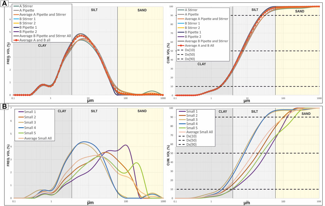
FIGURE 9. Volume frequency and cumulative frequency graphs for field sample C2 B0.4 S7. (A) Results from subsample A, pipette and stirrer, with average, and sub-sample B stirrer 1 and 2 as well as pipette 1 and 2, with average. An average for both sub-sample A and B combined is also shown. (B) Results for small sub-samples A, B, C, D, E, F, corresponding names small sample 1-5 and an average of all combined. For detailed results Supplementary Table S1, for p-values Supplementary Table S2.

Two large subsamples were disaggregated and analysed using the stirrer and pipette aliquot methods. Subsample A was processed as two aliquots: A stirrer and A pipette (Supplementary Table S1), all parameters measured were very similar except for the ASD which is significantly higher for the stirrer aliquot. Visual comparison of the stirrer and pipette aliquots from subsample A show very consistent results between the two methods (Figure 9) and the KS test provides a p-value of 0.6307 for these distributions. Four aliquots were extracted from subsample B: two stirrer aliquots and two pipettes. The parameters measured for this sub-sample are also very similar between aliquots. Accordingly, the P-vales are between 0.8888 and 1.000. Both subsample A and B are similar to the small samples E and F described above, and both aliquot sampling methods are consistent within each sample, again suggesting that either method can provide dependable results in mud-rich samples.

Comparison of Ultrasonic Bath to SELFRAG Disaggregation

Although the ultrasonic bath is a very useful method for disaggregating most samples, some well lithified samples with quartz cement (such as some from the Gottero Formation) were difficult or sometimes impossible to disaggregate through this method. A SELFRAG machine was utilized to disaggregate these more lithified samples. In order to establish how replicable the SELFRAG disaggregation method is, a sample from each of the 3 formations (Gottero, Marnoso-Arenacea and Castagnola), which vary in lithology and lithification, were compared to corresponding small subsamples disaggregated in the ultrasonic bath.

Method

In order to compare to the samples disaggregated using the ultrasonic bath method, three samples were disaggregated using the SELFRAG method (Figure 2). A significantly larger subsample was selected (roughly 25–100 g) and placed into the SELFRAG vessel and filled with water. The voltage (140 v) and number of discharges (50) was selected for the SELFRAG and the machine was activated. This was repeated until samples were sufficiently disaggregated, determined by feeling with a hand, and the sediment-water mixture was placed into the oven to dry. Dry samples were poured through a riffle splitter until they were deemed of sufficient size to be within obscuration limits for the Mastersizer 3000. This aliquot was then placed into a small centrifuge tube (15 ml) along with 10 ml of NaHMP and left for 24 h to deflocculate clays. Samples were checked under the microscope for disaggregation. These aliquots were then placed into the ultrasonic bath for a few minutes before measurement in the LPSA.

Results Castagnola Formation- VI 208 S2

Results from the three formations vary significantly. The poorly lithified formation (Castagnola Formation; Figures 10A, 11A), shows variable consistency between SELFRAG samples, with p values varying from 0.1317 to 1.0000. When compared to an average of small samples, SELFRAG samples S1-3 results are relatively similar in d_10, d₅₀ and d₉₀ values (Supplementary Table S1; Figure 11A). p-values between the small sample and SELFRAG samples range from 0.4938 to 0.6307 (Supplementary Table S2). These results suggest there is some inconsistency in the SELFRAG preparation method, but overall, they compare well to an average of small samples from the SELFRAG method (Figure 11A).

FIGURE 10

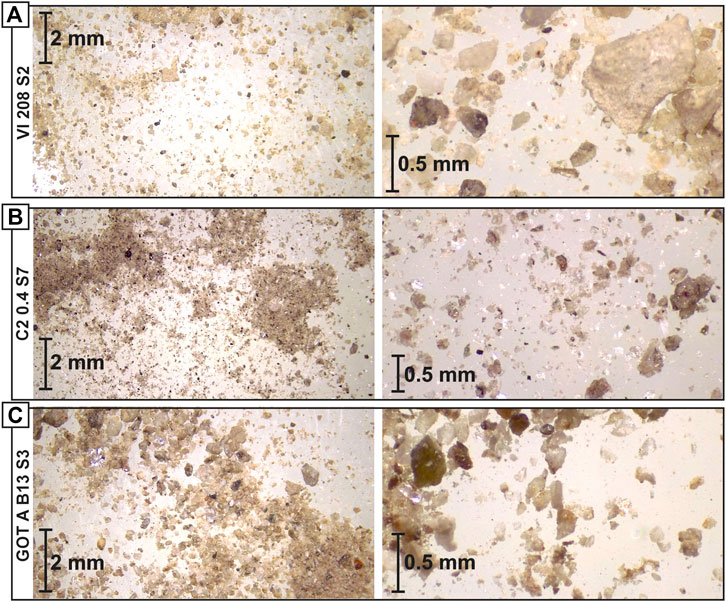
FIGURE 10. Photos taken under magnification of three samples disaggregated in SELFRAG, results shown in Figure 11. (A) Sample from Marnoso-Arenacea Formation (B) sample from Gottero Formation and (C) sample from Castagnola Formation. For data Supplementary Table S1.

FIGURE 11

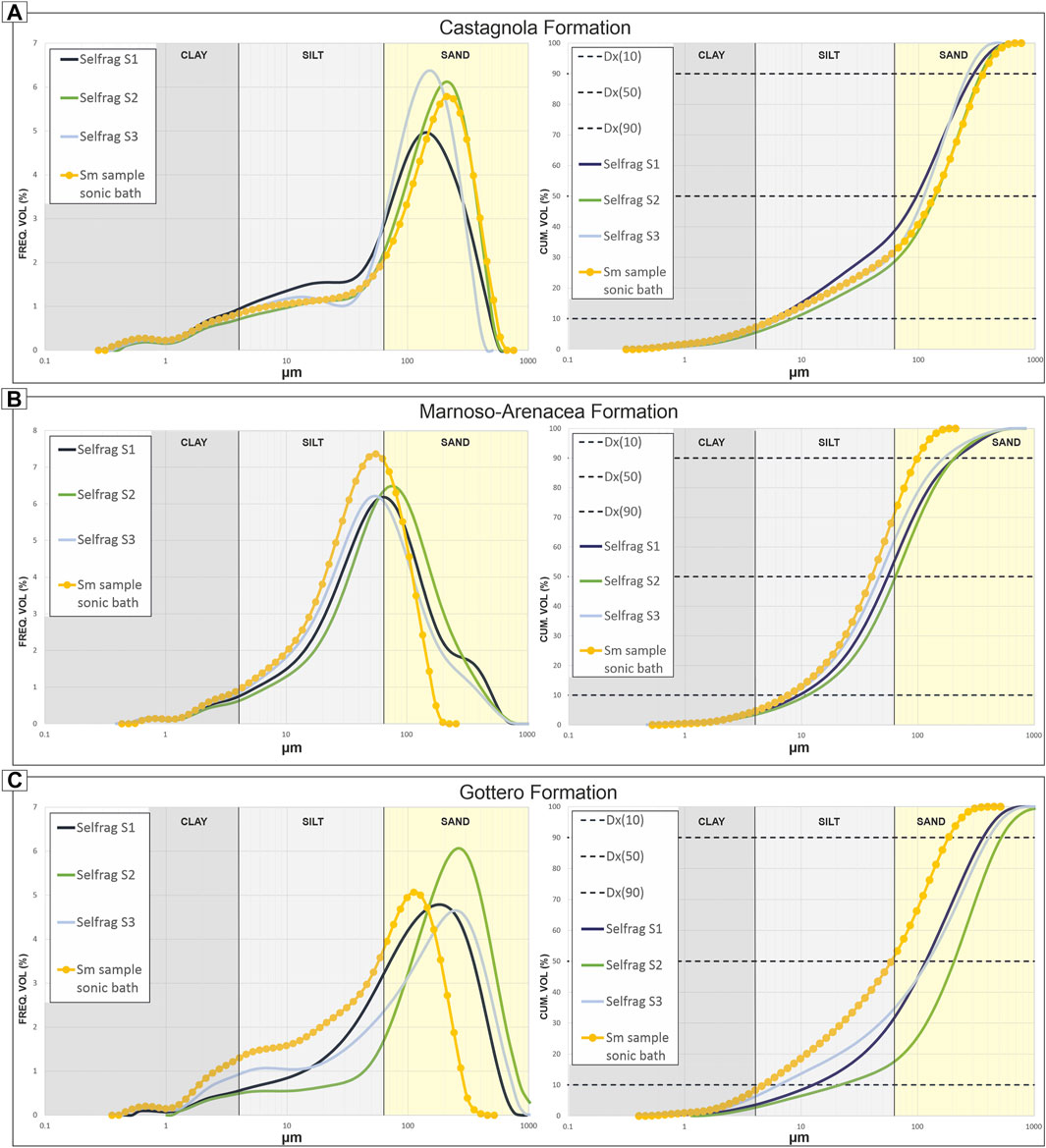
FIGURE 11. Volume frequency and cumulative frequency graphs for field sample showing comparison of samples disaggregated in SELFRAG and split with a riffle splitter (see text for details) and small subsample (yellow). (A) Example from the Castagnola formation, VI 208 S2 from the lower H1 division of a hybrid event bed. (B) Example from the Marnoso-Arenacea Formation, Location Coniale 2, Bed 0.4 (Amy and Talling, 2006), Sample 7, interpreted as part of the upper debritic portion of a hybrid event bed. (C) Example from the Gottero formation, GOT A B13 S3 from the matrix of a debritic portion, H3, of a hybrid event bed. For detailed results Supplementary Table S1, for p-values Supplementary Table S2.

Results Marnoso-Arenacea Formation- C2 B0.4 S7

The formation with an intermediate lithification (Marnoso-Arenacea Formation, Figures 10A, 11B), shows consistency between SELFRAG samples, with p-values between 0.8888 and 0.9999 (Supplementary Table S2).

When compared to an average of small sample, SELFRAG samples S1-3 shows more significant variation. The d₁₀ and d₅₀ values are relatively similar, particularly between the average small subsample and Selfrag S3 sample, but the d₉₀ values are significantly lower for the small sample as is the ASD (Figure 11B; Supplementary Table S1). Therefore, either the SELFRAG samples are not sufficiently disaggregated during processing, or the small subsample is not capturing the largest grain sizes in the field sample. p-values between the small sample and SELFRAG samples are 0.0878–0.3722.

Results Gottero Formation- GOT a B13 S3

The most lithified formation (Gottero Formation, Figures 10C, 11C), shows variability between SELFRAG samples 1–3, with p values varying from 0.0130 to 0.4938 (Supplementary Table S2). When comparing these SELFRAG samples to an average of small subsamples, d₅₀, d₉₀ and d₁₀ values for the SELFRAG samples are all significantly higher than for the small subsamples. Again, the higher d₉₀ value indicates that the SELFRAG samples are not sufficiently disaggregated during processing, or the small sample is not capturing the largest grain sizes in the field sample. The lower percentages of silt and clay volume for the SELFRAG samples, may be an indication that the SELFRAG is not sufficiently separating the finer portion from these well lithified samples. p-values between the small sample and SELFRAG samples show 0.0878–0.7695.

Recommendations

Overall, there is a general trend that the poorly lithified formation is efficiently disaggregated using the SELFRAG method, but the formation of intermediate lithification and the more lithified formation show more variability in statistical similarities. For the latter two formations, this trend is particularly noticeable in the d₉₀ values, which are significantly higher for the SELFRAG samples. This indicates that either the SELFRAG is not sufficiently disaggregating the most lithified samples or that the small samples from the most lithified formation are not accurately including the full range of grain sizes in the sample, particular the coarse grain-sizes. Further samples are needed to establish this. As this method could be highly beneficial for use with samples too cemented to be disaggregated in the sonic bath, this method is still recommended for use when necessary but must be used with caution and some trial for reproducibility.

Comparison to Thin Section Grain-Size Analysis

Method

Three samples are used to compare thin-section analysis with laser particle-size analysis: two from the Marnoso-Arenacea Formation and another from the Castagnola Formation (Figure 12). Three to five images were analysed for each thin section by measuring the long and short axes of individual grains. A grid was displayed over each image and each grain at the intersection of the vertical and horizontal lines was measured in order to assure grains were randomly selected. This measurement was undertaken manually by one single user for consistency of method.

FIGURE 12

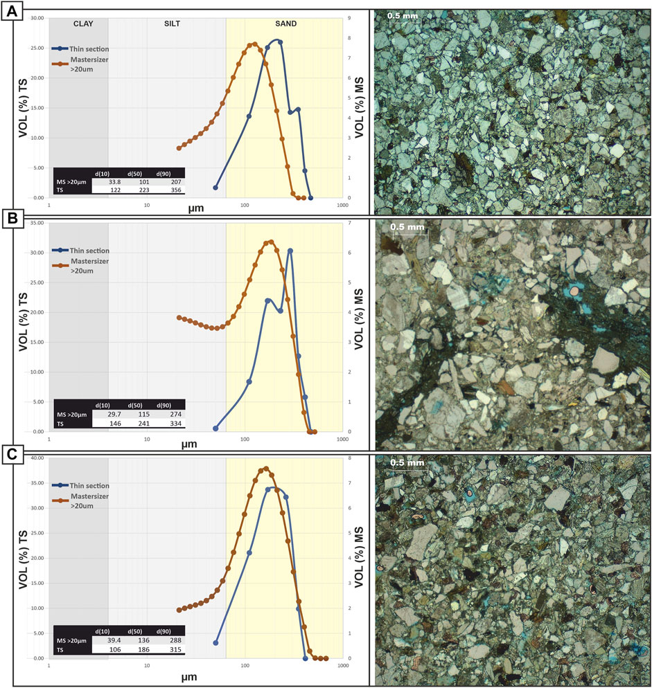
FIGURE 12. Volume frequency graphs from Mastersizer data compared to volume frequency graphs plotted from thin section measurement. The grain-size at the 10th, 50th and 90th percentile for the Mastersizer curve (MS) and from thin-section (TS) are shown in the inset graph. Data less than 20 µm were removed from the Mastersizer for more accurate comparison with thin section. Representative photos are shown for each thin section. (A) Example from the Marnoso-Arenacea Formation, location Coniale 1 (Figure 1B), bed 2, sample 1, collected from a sand-rich turbidite (Amy and Talling, 2006). (B) Example from the Marnoso-Arenacea Formation, location Coniale 2 (Figure 1), bed 1, sample 5B, collected from a clast within a hybrid event bed (Amy and Talling, 2006). (C) Example from the Castagnola Formation from log IV, bed 210 (Figure 1B), sample 5, collected from the sand-rich base of a hybrid event bed (Southern et al., 2015).

Grains from thin section are not a direct comparison to those from laser diffraction analysis because Mie theory gives results as volume equivalent spheres. Therefore, we can assume that a volume calculated from long and short axis measurement from the thin section will only show an approximation for any individual grain compared to the laser diffraction analysis. Due to the random cut of thin sections through grains, it is unlikely that the true long axis or short axis is captured. Long- and short-axes for 152–376 grains were measured for each thin section. To estimate the volume of each grain, the long axis was used as length, the short axis as the height and short axis again as the depth. The volumes were used to calculate a volume percentage of the whole for each grain in order to compare more directly with LPSA results. Grains were grouped into bins of 60 µm starting from 20 µm which was selected as the smallest reliable measurable value in thin-section. Results were then plotted at the midpoint for each distribution. There is some error involved in the comparison of volume distribution graphs between thin-section and LPSA results due to the large size of these bins.

Additionally, there is some human error involved in the manual measurement of grain-size in thin section. No grains under 20 µm were measured and grains under 100 µm are likely significantly underrepresented due to difficulty recognising and measuring these smaller grains. In order aid comparisons, LPSA results have been recalculated omitting grains <20 μm, therefore simulating measurements where finer grains are unmeasured. These LPSA curves are then compared to the thin section results (Figure 12). Unlike the LPSA samples, where calcite cement may have dissolved in the preparation process or be disaggregated, cement is still present in the thin sections. This cement is identified using cross-polarised light and therefore omitted from any measurement.

Results of Comparison

Thin Section 1- Marnoso-Arenacea Formation (Bed 2, Turbidite).

This section is the from the Marnoso-Arenacea Formation, location Coniale 1 (Figure 1B), bed 2, sample 1, collected from a sand-rich turbidite (Amy and Talling, 2006). Grain size curves and d₁₀, d₅₀ and d₉₀ values are shown in Figure 12A.

Description

Grain size curves are broadly similar for the coarser values, although a distinct finer tail can be shown in the LPSA data, which is not seen in the thin section data (Figure 12A). The thin section curve is shifted coarser by 60 µm for the silt to very fine sand component and 10 µm for the fine to coarse sand component, with the peak shifting 100 µm coarser for the thin section data (from very fine to fine sand). The d₁₀, d₅₀ and d₉₀ values are all significantly higher for the thin section compared to the LPSA (Figure 12A). The d₁₀ value varies from coarse silt in the LPSA results to very fine sand in thin section. The d₅₀ value varies from very fine sand in the LPSA results to fine sand in the thin section. The d₉₀ value varied from fine sand in the LPSA results to medium sand in the thin section.

Thin Section 2- Marnoso-Arencea Formation, Clast (Bed 1, Hybrid Event Bed).

This section is the from the Marnoso-Arenacea Formation, location Coniale 2 (Figure 1B), bed 1, sample 5B, collected from a rip-up clast within a hybrid event bed (Amy and Talling, 2006). Grain size curves and d₁₀, d₅₀ and d₉₀ values are shown in Figure 12B.

Description

The grain size curves are broadly similar shapes for the coarser grain-size fraction (>100 µm) but differ significantly for the finer fraction (<100 µm). The data from the LPSA and the thin section indicate that this sample has a larger portion of clay and silt grains compared to the previous sample (Figure 12A). The finer tail and significant silt portion shown in the LPSA curve are not seen in the thin section curve. The grain sizes greater than 300 µm are a similar volume distribution for both the LPSA and thin section curves. A double peak is seen in the thin section curve that is not apparent in the LPSA curve. The tallest peak is around 100 µm coarser for the thin-section curve (from fine to medium sand). The d₁₀, d₅₀ and d₉₀ values are all significantly higher for the thin section compared to the LPSA, with the d₁₀ value varying from medium silt in the LPSA to fine sand in thin section and the d₅₀ value varying from very fine sand in the LPSA to fine sand in the thin section. The d₉₀ is medium sand for both the LPSA and the thin section curves.

Thin Section 3- Castagnola Formation (Bed 210, Hybrid Event Bed).

This sample is from the Castagnola Formation from log IV, bed 210 (Figure 1B), sample 5, collected from the sand-rich base of a hybrid event bed (Southern et al., 2015). Graph of data and d₁₀, d₅₀ and d₉₀ values are shown in Figure 12C.

Description

The LPSA and thin-section curves are broadly similar shapes for the coarser portion, with the thin section missing the finer tail present in the LPSA curve (Figure 12C). Both curves have peaks at fine sand grain sizes. Like the previous examples, the d₁₀, d₅₀ and d₉₀ values are all higher in the thin section analysis, although they are most similar out of all three examples. The d₁₀ value varies from coarse silt in the LPSA to very fine sand in thin section. The d₅₀ value is fine sand for both the LPSA and thin section curve. The d₉₀ is medium sand for both the LPSA and the thin section curve.

Interpretation

Overall, there are significant differences between the LPSA and thin section grain-size distributions. Most importantly, the thin section curves are missing the finer tail present in the LPSA data and correspondingly all graphs show significantly coarser d₁₀, d₅₀ and d₉₀ values. Major differences between LPSA and thin section results could arise from difficulty in measuring small grains in thin section, volume approximation methods, spherical grain assumptions made by the LPSA, and error introduced by sample preparation prior to LPSA analysis. The higher d₁₀ values likely result from the difficulty in accurate measurement of silt-sized grains and the smaller sample size of grains measured in thin section. This is most notable in thin section 2 (Figure 12B), which is the most clay/silt-rich (according to the LPSA data and images). This in turn affects the d₅₀ and d₉₀ values, with distribution weighted more towards the coarser grains in the thin section. Additionally, the method used to create a volume approximation could be influencing the result. Using the long axis and the short axis twice is a best estimate and may not result in realistic volumes for each grain. The double peak apparent in the thin section 2 curve (Figure 12B) is likely a result of the lower number of grains counted (262) compared to thousands in the LPSA as well as the grouping of samples into 60 µm bins. The angularity of the grains is likely not a large factor, as all three samples appear to be of similar angularity (sub-angular to sub-rounded, Figure 12). There is a possibly that the finer-grained LPSA values, both the increased fine-grained component and the decreased maximum grain size, could result from sample breakdown beyond grain boundaries in the preparation process for the LPSA, but due to the replicability of samples in the LPSA this is unlikely.

Despite all effort being made to take field samples within proximity of each other, some natural variation between samples is possible, particularly from thin-section 2 (Figure 12B) which is from a clast within a hybrid event bed. Due to the large sample size needed to make a thin section, samples can be estimated as only being within the same 20 cm section of each bed. It is therefore possible that, like for the large and small subsamples described above, some differences between thin section and LPSA curves represent real variation between samples.

The comparison between thin section and LPSA results suggest that care should be taken when comparing grain-size analysis methods to one another. While trends within a given method may be meaningful, specific values of d₁₀, d₅₀, or d₉₀ may vary significantly between methods. Thin sections in this study underestimate the silt-sized fraction and were unable to measure clay fraction, which results in a coarse-grained shift in cumulative grain size values (e.g., d₅₀).

Discussion and Recommendations

Aliquot Methods

Overall, aliquots measured using the stirrer method were more replicable than the pipette method. This is likely due to the mechanisation of the stirrer being more consistent than manual pumping with the pipette when dispersing grains into suspension. However, individual aliquots can show inaccuracies due to a few anomalously large grains. One way to avoid this potential error is to take a large subsample and continue to extract aliquots until the entire sample has been measured. This is the most accurate representation of grain size available because using all of a large subsample allows for more individual grains to be measured. By averaging multiple subsamples there is also less risk of an anomalous aliquot or measurement error interfering with the dataset. However, using a very large number of aliquots (>6) will significantly increase processing time.

Large Subsamples or Small Subsamples?

Although larger subsamples give more representative data, smaller subsamples negate any aliquot sampling error and are accurate when compared to an average of large subsamples in most cases. Overall, small subsamples are significantly less time consuming and were sufficiently accurate for the samples in this study. However, it is advised that multiple small samples are measured for a given field sample to account for any potential heterogeneity.

Speed and Accuracy Ultrasonic Bath Method

Overall, samples were highly replicable and therefore the ultrasonic bath method is reliable. The speed at which samples could be processed was a few minutes for the sample preparation, 20 min to 1 h in the ultrasonic bath, 24 h for clay deflocculation, 3 min to run through the Mastersizer 3000 and 1 min for cleaning in between samples. As 10s of samples could be placed in the ultrasonic bath together and left to deflocculate overnight, it was possible to get through approximately 30 samples per day.

Speed and Accuracy SELFRAG Method

Disaggregating samples using the SELFRAG method was much more time consuming than the ultrasonic bath. Approximately 5 samples could be processed in the SELFRAG per day and left to dry overnight. These were then subsampled in the riffle splitter the following day and left in a 0.5% NaHMP solution over a second night before being measured in the LPSA (Figure 2). The results suggest that the SELFRAG method was not fully disaggregating clasts in the most lithified formations, and because the least lithified formations can be more easily disaggregated in the ultrasonic bath method, it is not recommended to use the SELFRAG method without further testing. The SELFRAG method could potentially be used in conjunction with the ultrasonic bath method, however further testing is required.

Comparison With Thin Section

There are many issues with the direct comparison between laser diffraction methods and thin section for grain-size analysis. Most thin section studies use the long axes measured in a 2D thin section, which does not represent the true longest axes of the original grains and will therefore likely underestimate the size of larger sand grains in most cases (Smith, 1966; Sahu, 1968; Johnson, 1994), but will also not accurately capture clay and silt grains. In this study, we attempted to offset this issue through calculating an artificial volume. Other methods for converting 2D to 3D grain-size distributions have been developed (e.g., Heilbronner and Barrett, 2014), but these are not straightforward. In general, results show an overestimation of grain size using thin section analysis, which could be due to using the short axis as both the height and depth, potentially overestimating the z-axis.

Recent work by Maithel et al. (2019) comparing laser diffraction and thin section analysis for sandstones found a good comparison between their results, with the laser diffraction being slightly coarser overall, which was expected because they used the long-axis method in thin section. The difference between the medians for thin-section and laser-diffraction data sets (based on average grain sizes for each sample) was 33.7 µm. They hypothesised the difference could be due to numerous variables such as natural sample variation and sources of error or potentially due to measurement of quartz overgrowths in disaggregated samples. The more consistent relationship between laser diffraction and thin-section methods by Maithel et al. (2019) compared to this study is likely to due to the removal of fines in their sample preparation stage. Silt particles are underrepresented in thin section measurements and clay was not measured at all. Despite this, Maithel et al. (2019) did also find issues relating to disaggregation quality and correspondence with thin section samples, like those demonstrated by the SELFRAG samples in this study. Overall Maithel et al. (2019) conclude that consistency between their laser diffraction and thin section results confirms the robustness of both methods for textural analysis, which may be the case when using only sand-sized grains, but which this study demonstrates is not the case when including silt and clay.

Issues With Clays

In comparison with thin-section analysis, the LPSA was more accurate in documenting the presence of silt and was able to measure clay particles. Although this is likely missing in the thin section analysis due to the limitations of the method, some studies (Buurman, et al., 1997; Buurman, et al., 2001) have shown that laser diffraction methods can inaccurately measure the size of clay and fine silt fractions of a sample. Work carried out using soil profiles (Bah, et al., 2009), suggested that the relationship between clay determined by settling method (e.g., sieve-hydrometer method) and clay determined by laser diffraction analysis may depend on the physical properties of the clay. This can be due to the heterogeneity of sediment particle density and the deviation of particle shapes from sphericity (Bah, et al., 2009). Therefore, in the LPSA, an irregular shaped soil particle reflects a cross-sectional area greater than that of a sphere having the same volume. Thus, particles are assigned to larger size fractions of the particle size distribution and the clay fraction is underestimated. Non-spherical particles in settling methods have longer settling times than their equivalent spheres, which results in an overestimation of the clay fraction. This is likely only a minor consideration when mixed sand, silt, clay samples are used, but should be taken into consideration when exact clay volumes are more pertinent to the study.

What Are the Limits of This Method Overall?

Overall, this study found that the laser diffraction grain size analysis with the Malvern Mastersizer 3000 is generally replicable and reliable for mixed sand-silt-clay samples of varying distributions. The small subsample method is the most time efficient sub-sampling method for analysing datasets with hundreds of field samples, but care needs to be taken to re-run samples that appear anomalous. Despite the accuracy and speed of the small subsample method, there are still some drawbacks. Natural samples will almost always vary spatially, which will add error to the dataset. Despite this drawback, sieving and thin section analysis will also have issues with subsampling and therefore this is a source of error that cannot be completely negated. There is a certain amount of specialist equipment required for laser diffraction grain-size analysis, but this method may be more cost effective when compared to thin section preparation in the long run or labour in processing sieved samples. Users can be trained in the methods described in this study (Figure 2) within a day. Ultrasonic baths are cheap and easily accessible. The SELFRAG on the other hand is a large, expensive, and specialised piece of equipment, which requires more training and has been shown in this study to give variable results. It is therefore not recommended unless access is already available.

Conclusion

This study demonstrated that it is possible to produce a reliable and repeatable workflow for disaggregating ancient mudstone and sandstone utilizing an ultrasonic bath for variably cemented samples. This study also demonstrates these techniques are possible on moderately-cemented rocks up to Cretaceous age, opening the opportunity for laser-diffraction grain size analysis on ancient sedimentary rocks. The most efficient samples to run were “small” (0.2–2 g) subsamples, which were found to be sufficiently accurate when compared to an average of “large” (5—10 g) subsamples. Multiple small samples can be run relatively quickly to rule out anomalous results. Alternatively, large subsamples, which are presumably more representative of the entire field sample, can be measured using aliquots obtained with either the pipette or stirrer method. In argillaceous samples, the “agitated” pipette method and “centre” stirrer method were found to be replicable, and the stirrer provided more consistent results in general. In sand-rich samples, the pipette method is slightly skewed towards coarser grain sizes and the stirrer method is slightly skewed towards finer grain sizes, however each method was internally precise.

The SELFRAG method for disaggregation was possible, but due to the large amount of sample needed for this method, drying and splitting the dry sample with a riffle-splitter was time consuming. This method is therefore only suitable with a small number of field samples. Moreover, there were potentially some remaining aggregate grains for the samples from moderately lithified and most lithified formations. Therefore, this method may need to be further developed or combined with the ultrasonic bath method to be fully reliable. However, the SELFRAG does have the potential to allow disaggregation of older and more well-cemented sedimentary rocks.

When compared to thin section analysis, laser diffraction results showed significant differences, including LPSA results being finer due to a more accurate measurement of the silt portion and inclusion of the clay portion of samples. Grain-size of the sand portion was over-estimated in the thin-section analysis, potentially due to the overestimation of the unmeasured z-axis of grains.

Despite some issues, the ultrasonic bath method of disaggregation and measurement using the Mastersizer 3000 has made it possible to measure accurate grain size distributions for hundreds of samples in a reasonable amount of time. Therefore, by following the workflow outlined in this study and using the processing techniques most suitable for the dataset, it is possible to greatly expand the amount of quantitative grain-size datasets for ancient siliciclastic sedimentary rocks.

Data Availability Statement

The original contributions presented in the study are included in the article/Supplementary Material, further inquiries can be directed to the corresponding author.

Author Contributions

HB and ES conceived and designed the study, underwent fieldwork and collected samples. HB, ES and MM ran the experiments in the laboratory. HB wrote the first draft of the manuscript, ES reviewed and redrafted manuscript. All authors contributed to manuscript revision, read and approved the submitted version.

Funding

This work was carried out with funding from the Queen’s University postdoctoral fund. Supportive funding was used from the Natural Sciences and Engineering Research Council of Canada (NSERC), RGPIN-2019-04760 and Research Initiation Grant awarded to ES from Queen’s University.

Conflict of Interest

The authors declare that the research was conducted in the absence of any commercial or financial relationships that could be construed as a potential conflict of interest.

Publisher’s Note

All claims expressed in this article are solely those of the authors and do not necessarily represent those of their affiliated organizations, or those of the publisher, the editors and the reviewers. Any product that may be evaluated in this article, or claim that may be made by its manufacturer, is not guaranteed or endorsed by the publisher.

Acknowledgments

The Authors would like to thank Marco Patacci for introducing us to the Castagnola and Gottero field areas where samples were collected, and Esther Sumner for providing data on the Marnoso-Arenacea field area. We would also like to thank Michele Malavolta, Yvonne Spychala and Sarah Cobain for assistance in the field, Gillian Ivey and Valentin Zuchuat for assistance in the Lab, Steve Beyer at Queens University for cutting thin sections and assistance with the SELFRAG and Pam Frail at Acadia University for preparation of thin section. A big thank you to Bob Dalrymple for providing the funds for the Mastersizer 3000. Thank you to Peir Pufahl for assistance and use of lab equipment. Finally, thank you to Megan Baker, Chris Stevenson, Assoc. Prof. Roberto Tinterri and RS for their insightful and helpful reviews. We acknowledge the support of the Natural Sciences and Engineering Research Council of Canada (NSERC), RGPIN-2019-04760.

Supplementary Material

The Supplementary Material for this article can be found online at: https://www.frontiersin.org/articles/10.3389/feart.2022.820866/full#supplementary-material

References

Abbate, E., and Sagri, M. (1970). The Eugeosynclinal Sequences. Sediment. Geology. 4, 251–340. doi:10.1016/0037-0738(70)90018-7

CrossRef Full Text | Google Scholar

Amy, L. A., and Talling, P. J. (2006). Anatomy of Turbidites and Linked Debrites Based on Long Distance (120 X 30 Km) Bed Correlation, Marnoso Arenacea Formation, Northern Apennines, Italy. Sedimentology 53 (1), 161–212. doi:10.1111/j.1365-3091.2005.00756.x

CrossRef Full Text | Google Scholar

Amy, L. A., Talling, P. J., Sumner, E. J., and Malgesini, G. (2016). Current-aligned Dewatering Sheets and 'enhanced' Primary Current Lineation in Turbidite Sandstones of the Marnoso-Arenacea Formation. Sedimentology 63 (5), 1260–1279. doi:10.1111/sed.12260

CrossRef Full Text | Google Scholar

Andreola, F., Castellini, E., Manfredini, T., and Romagnoli, M. (2004). The Role of Sodium Hexametaphosphate in the Dissolution Process of Kaolinite and Kaolin. J. Eur. Ceram. Soc. 24 (7), 2113–2124. doi:10.1016/s0955-2219(03)00366-2

CrossRef Full Text | Google Scholar

Andreola, F. (2006). Effect of Sodium Hexametaphosphate and Ageing on the Rheological Behaviour of Kaolin Dispersions. Appl. Clay Sci. 31 (1-2), 56–64. doi:10.1016/j.clay.2005.08.004

CrossRef Full Text | Google Scholar

Andreoni, G., Galbiati, B., Maccabruni, A., and Vercesi, P. (1981). Stratigrafia e paleogeografia deidepositi oligocenici sup. – miocenici inf. nell’estremita’ orientale del bacino ligure-piemontese. Riv. Ital. Paleontol. Stratigr. 87, 245–282.

Google Scholar

Andres, U. (2010). Development and Prospects of mineral Liberation by Electrical Pulses. Int. J. Mineral Process. 97 (1-4), 31–38. doi:10.1016/j.minpro.2010.07.004

CrossRef Full Text | Google Scholar

Argnani, A., and Lucchi, F. R. (2001). The Apennines and Adjacent Mediterranean Basins. Dordrecht: Springer.

Google Scholar

Bah, A. R., Kravchuk, O., and Kirchhof, G. (2009). Fitting Performance of Particle-Size Distribution Models on Data Derived by Conventional and Laser Diffraction Techniques. Soil Sci. Soc. Am. J. 73 (4), 1101–1107. doi:10.2136/sssaj2007.0433

CrossRef Full Text | Google Scholar

Barrett, P., and Anderson, J. (2000). Grain Size Analysis of Samples from CRP-2/2A. Terra Antarctica 7 (3), 373–378.

Google Scholar

Blott, S. J., Croft, D. J., Pye, K., Saye, S. E., and Wilson, H. E. (2004). “Particle Size Analysis by Laser Diffraction,” Geol. Soc. Lond. Spec. Publications in Forensic Geoscience: Principles, Techniques and Applications. Editors K. Pye, and D. J. Croft (London: The Geological Society of London), 232, 63–73. doi:10.1144/gsl.sp.2004.232.01.08

CrossRef Full Text | Google Scholar

Bralower, T., Eccles, L., Kutz, J., Yancey, T., Schueth, J., Arthur, M., et al. (2010). Grain Size of Cretaceous-Paleogene Boundary Sediments from Chicxulub to the Open Ocean: Implications for Interpretation of the Mass Extinction Event. Geology 38 (3), 199–202. doi:10.1130/g30513.1

CrossRef Full Text | Google Scholar

Buller, A. T., and McManus, J. (1972). Modes of Turbidite Deposition Deduced from Grain-Size Analyses. Geol. Magazine 109(6), 491–500.

CrossRef Full Text | Google Scholar

Buurman, P., Pape, T., and Muggler, C. C. (1997). Laser Grain-Size Determination in Soil Genetic Studies 1. Practical Problems. Soil Sci. 162 (3), 211–218. doi:10.1097/00010694-199703000-00007

CrossRef Full Text | Google Scholar

Buurman, P., Pape, T., Reijneveld, J. A., De Jong, F., and Van Gelder, E. (2001). Laser-diffraction and Pipette-Method Grain Sizing of Dutch Sediments: Correlations for fine Fractions of marine, Fluvial, and Loess Samples. Neth. J. Geosciences 80 (2), 49–57. doi:10.1017/s0016774600022319

CrossRef Full Text | Google Scholar

Cavanna, F., Di Giulio, A., Galbiati, B., Mosna, S., Perotti, C. R., and Pieri, M. (1989). Carta geologica dell'estremità orientale del Bacino Terziario Ligure Piemontese. Atti Ticinesi Sc. Terra, 32.

Chakravarti, I. M., Laha, R. G., and Roy, J. (1967). Handbook of Methods of Applied Statistics, Volume I John Wiley and Sons, Hoboken, pp. 392-394

Chayes, F. (1950). On the Bias of Grain-Size Measurements Made in Thin Section. J. Geology. 58 (2), 156–160. doi:10.1086/625716

CrossRef Full Text | Google Scholar

Cheetham, M. D., Keene, A. F., Bush, R. T., Sullivan, L. A., and Erskine, W. D. (2008). A Comparison of Grain-Size Analysis Methods for Sand-Dominated Fluvial Sediments. Sedimentology 55, 1905–1913. doi:10.1111/j.1365-3091.2008.00972.x

CrossRef Full Text | Google Scholar

Chilingar, G. V. (1952). Study of the Dispersing Agents. J. Sediment. Res. 22 (4), 229–233. doi:10.2110/jsr.22.229

CrossRef Full Text | Google Scholar

Di Giulio, A., and Galbiati, B. (1993). Escursione nell’estremitaorientale del Bacino Terziario Piemontese. Interazione tettonica-eustatismo nella sedimentazione di un bacino tardo-post orogenico. 3 Convegno del Gruppo Informale di Sedimentologia del CNR. Dip. di Scienza della Terra, Università di Pavia, Salica Term, 1–28.

Google Scholar

Di Stefano, C., Ferro, V., and Mirabile, S. (2010). Comparison between Grain-Size Analyses Using Laser Diffraction and Sedimentation Methods. Biosyst. Eng. 106, 205–215. doi:10.1016/j.biosystemseng.2010.03.013

CrossRef Full Text | Google Scholar

Edwards, A. P., and Bremner, J. M. (1967). Dispersion of Soil Particles by Sonic Vibration1. J. Soil Sci. 18, 47–63. doi:10.1111/j.1365-2389.1967.tb01487.x

CrossRef Full Text | Google Scholar

Fernlund, J., Zimmerman, R., and Kragic, D. (2007). Influence of Volume/mass on Grain-Size Curves and Conversion of Image-Analysis Size to Sieve Size. Eng. Geology. 90 (3-4), 124–137. doi:10.1016/j.enggeo.2006.12.007

CrossRef Full Text | Google Scholar

Fonnesu, M., Felletti, F., Haughton, P. D., Patacci, M., and McCaffrey, W. D. (2018). Hybrid event bed character and distribution linked to turbidite system sub‐environments: The North Apennine Gottero Sandstone (North‐West Italy). Sedimentology 65(1), 151–190.

CrossRef Full Text | Google Scholar

Fonnesu, M., Patacci, M., Haughton, P. D., Felletti, F., and McCaffrey, W. D. (2016). Hybrid Event Beds Generated by Local Substrate Delamination on a Confined-Basin Floor. J. Sediment. Res. 86(8), 929–943.

CrossRef Full Text | Google Scholar

Francus, P. (1999). Using Image Analysis to Estimate Quantitatively Some Microstructural Parameters of Detrital Sediments. Geologica Belgica 2, 173–180.

Google Scholar

Friedman, G. M. (1958). Determination of Sieve-Size Distribution from Thin-Section Data for Sedimentary Petrological Studies. J. Geology. 66 (4), 394–416. doi:10.1086/626525

CrossRef Full Text | Google Scholar

Gee, G. W., and Bauder, J. W. (1986). “Particle‐size Analysis,” in Methods of Soil Analysis: Part 1 Physical and Mineralogical Method. Editor A. Klute (Madison, Wisconsin, USA: the American Society of Agronomy, Inc. Soil Science Society of America, Inc.).

Google Scholar

Greenman, N. N. (1951). The Mechanical Analysis of Sediments from Thin-Section Data. J. Geology. 59 (5), 447–462. doi:10.1086/625889

CrossRef Full Text | Google Scholar

Harrell, J., and Eriksson, K. (1979). Empirical Conversion Equations for Thin-Section and Sieve Derived Size Distribution Parameters. J. Sediment. Petrology 49, 273–280. doi:10.1306/212f7711-2b24-11d7-8648000102c1865d

CrossRef Full Text | Google Scholar

Heilbronner, R., and Barrett, S. (2014). Spatial Distributions. Image Analysis in Earth Sciences eds. Heilbronner, R. and Barrett, S. Springer, Berlin, Heidelberg, 351–368. doi:10.1007/978-3-642-10343-8_18

CrossRef Full Text | Google Scholar

Haughton, P. D. W., Barker, S. P., and McCaffrey, W. D. (2003). 'Linked' Debrites in Sand-Rich Turbidite Systems - Origin and Significance. Sedimentology 50 (3), 459–482. doi:10.1046/j.1365-3091.2003.00560.x

CrossRef Full Text | Google Scholar

Haughton, P., Davis, C., McCaffrey, W., and Barker, S. (2009). Hybrid Sediment Gravity Flow Deposits‐Classification, Origin And Significance. Marine Petrol. Geol. 26(10), 1900–1918.

CrossRef Full Text | Google Scholar

Hayton, S., Nelson, C. S., Ricketts, B. D., Cooke, S., and Wedd, M. W. (2001). Effect of Mica on Particle-Size Analyses Using the Laser Diffraction Technique. J. Sediment. Res. 71 (3), 507–509. doi:10.1306/2dc4095b-0e47-11d7-8643000102c1865d

CrossRef Full Text | Google Scholar

Hodgson, D. M. (2009). Distribution and Origin of Hybrid Beds in Sand-Rich Submarine Fans of the Tanqua Depocentre, Karoo Basin, South Africa. Mar. Pet. Geology. 26 (10), 1940–1956. doi:10.1016/j.marpetgeo.2009.02.011

CrossRef Full Text | Google Scholar

Ito, M. (2008). Downfan Transformation from Turbidity Currents to Debris Flows at a Channel-To-Lobe Transitional Zone: the Lower Pleistocene Otadai Formation, Boso Peninsula, Japan. J. Sediment. Res. 78 (10), 668–682. doi:10.2110/jsr.2008.076

CrossRef Full Text | Google Scholar

Jiang, Z., and Liu, L. a. (2011). A Pretreatment Method for Grain Size Analysis of Red Mudstones. Sediment. Geology. 241, 13–21. doi:10.1016/j.sedgeo.2011.09.008

CrossRef Full Text | Google Scholar

Johnson, M. R. (1994). Thin Section Grain Size Analysis Revisited. Sedimentology 41, 985–999. doi:10.1111/j.1365-3091.1994.tb01436.x

CrossRef Full Text | Google Scholar

Konert, M., and Vandenberghe, J. (1994). Comparison of Laser Grain Size Analysis with Pipette and Sieve. Sedimentology 44, 523–535. doi:10.1046/j.1365-3091.1997.d01-38.x

CrossRef Full Text | Google Scholar

Kong, M., Bhattacharya, R. N., James, C., and Basu, A. (2005). A Statistical Approach to Estimate the 3D Size Distribution of Spheres from 2D Size Distributions. Geol. Soc. America Bull. 117, 244–249. doi:10.1130/b25000.1

CrossRef Full Text | Google Scholar

Krumbein, W. C. (1935). Thin-section Mechanical Analysis of Indurated Sediments. J. Geology. 43 (5), 482–496. doi:10.1086/624330

CrossRef Full Text | Google Scholar

Loope, D. B., Elder, J. F., and Sweeney, M. R. M. (2012). Downslope Coarsening in Aeolian Grainflows of the Navajo Sandstone. Sediment. Geology. 265-266, 156–162. doi:10.1016/j.sedgeo.2012.04.005

CrossRef Full Text | Google Scholar

Lucchi, F. R., and Valmori, E. (1980). Basin-wide Turbidites in a Miocene, Over-supplied Deep-Sea plain: a Geometrical Analysis. Sedimentology 27 (3), 241–270. doi:10.1111/j.1365-3091.1980.tb01177.x

CrossRef Full Text | Google Scholar

Maithel, S. A., Brand, L. R., and Whitmore, J. H. (2019). A Methodology for Disaggregation and Textural Analysis of Quartz-Cemented Sandstones. J. Sediment. Res. 89 (7), 599–609. doi:10.2110/jsr.2019.35

CrossRef Full Text | Google Scholar

Malesani, P. (1966). Ricerche Sulle Arenarie, XV; L’Arenaria Superiore. Rendiconti della Società Italiana di Mineralogia e Petrologia 22, 113–175.

Google Scholar

Marroni, M. a. P. N. (1990). The Age of the Ophiolite Sedimentary Cover from the Mt. Gottero Unit (Internal Ligurid Units, Northern Apennines): New Data from Calcareous Nannofossils. Ofioliti 15, 251–267.

Google Scholar

Marroni, M., Meneghini, F., and Pandolfi, L. (2004). From Accretion to Exhumation in a Fossil Accretionary Wedge: a Case History from Gottero Unit (Northern Apennines, Italy). Geodinamica Acta 17, 41–53. doi:10.3166/ga.17.41-53

CrossRef Full Text | Google Scholar

Mazzullo, J., and Kennedy, S. K. (1985). Automated Measurement of the Nominal Sectional Diameters of Individual Sedimentary Particles. J. Sediment. Res. 55 (4), 593–595. doi:10.2110/55.4.593

CrossRef Full Text | Google Scholar

Muzzi Magalhaes, P., and Tinterri, R. (2010). Stratigraphy and Depositional Setting of Slurry and Contained (Reflected) Beds in the Marnoso-Arenacea Formation (Langhian-Serravallian) Northern Apennines, Italy. Sedimentology 57 (7), 1685–1720. doi:10.1111/j.1365-3091.2010.01160.x

CrossRef Full Text | Google Scholar

Nilsen, T., and Abbate, E. (1984). Turbidite Facies and Facies Associations of Cretaceous and Paleocene Gottero sandstone, Northern Italy. AAPG Bull. 68 (4), 512–513. doi:10.1306/ad461061-16f7-11d7-8645000102c1865d

CrossRef Full Text | Google Scholar

Pandolfi, L. (1997). Stratigrafia ed Evoluzione Strutturale delle Succession Torbiditiche Cretacee della Liguria Orientale (Appennino Settentrionale). PhD thesis, Università di Pisa, 175 pp.

Parea, G. C. (1965). Evoluzione Della Parte Settentrionale Della Geosinclinale Appenninica dall'Albiano all'Eocene Superiore. Atti e Memorie della Accademia Nazionale di Scienze, Lettere, e Arti, Modena 6 (7), 97.

Google Scholar

Passerini, P., and Pirini, C. (1964). Microfaune paleoceniche nella formazione dell’Arenaria del M. Ramaceto e degli Argilloscisti di Cichero. Societa Geologica Italiana Bolletin 83, 211–218.

Google Scholar

Patacci, M., Marini, M., Felletti, F., Di Giulio, A., Setti, M., and McCaffrey, W. (2020). Rigin of Mud in Turbidites and Hybrid Event Beds: Insight from Ponded Mudstone Caps of the Castagnola Turbidite System (north‐west Italy). Sedimentology 67. doi:10.1111/sed.12713

CrossRef Full Text | Google Scholar

Persson, A.-L. (1998). Image Analysis of Shape and Size of fine Aggregates. Eng. Geology. 50, 177–186. doi:10.1016/s0013-7952(98)00009-x

CrossRef Full Text | Google Scholar

Rendigs, R. R., and Commeau, J. A. (1987). Effects of Disaggregation on a fine-grained marine Mud by Two Ultrasonic Devices. J. Sediment. Res. 57 (4), 786–787. doi:10.1306/212f8c51-2b24-11d7-8648000102c1865d

CrossRef Full Text | Google Scholar

Resentini, A., AndÒ, S., and Garzanti, E. (2018). Quantifying Roundness of Detrital Minerals by Image Analysis: Sediment Transport, Shape Effects, and Provenance Implications. J. Sediment. Res. 88 (2), 276–289. doi:10.2110/jsr.2018.12

CrossRef Full Text | Google Scholar

Rosenfeld, M. A., Jacobsen, L., and Ferm, J. C. (1953). A Comparison of Sieve and Thin-Section Technique for Size Analysis. J. Geology. 61 (2), 114–132. doi:10.1086/626060

CrossRef Full Text | Google Scholar

Sahu, B. (1968). The Determination of the Grain-Size Distribution of a Spherical Granular Material Embedded in Matrix. Sedimentology 10, 293–309. doi:10.1111/j.1365-3091.1968.tb01107.x

CrossRef Full Text | Google Scholar

Saini-Eidukat, B., and Weiblen, P. W. (1996). A New Method of Fossil Preparation, Using High-Voltage Electric Pulses. Curator 39, 139–144. doi:10.1111/j.2151-6952.1996.tb01085.x

CrossRef Full Text | Google Scholar

Seelos, K., and Sirocko, F. (2005). RADIUS - Rapid Particle Analysis of Digital Images by Ultra-high-resolution Scanning of Thin Sections. Sedimentology 52 (3), 669–681. doi:10.1111/j.1365-3091.2005.00715.x

CrossRef Full Text | Google Scholar

Smith, R. E. (1966). Grain Size Measurement in Thin Section and in Grain Mount. J. Sediment. Res. 36, 841–843. doi:10.1306/74d715aa-2b21-11d7-8648000102c1865d

CrossRef Full Text | Google Scholar

Southern, S. J., Patacci, M., Felletti, F., and McCaffrey, W. D. (2015). Influence of Flow Containment and Substrate Entrainment upon sandy Hybrid Event Beds Containing a Co-genetic Mud-Clast-Rich Division. Sediment. Geology. 321, 105–122. doi:10.1016/j.sedgeo.2015.03.006

CrossRef Full Text | Google Scholar

Sperazza, M., Moore, J. N., and Hendrix, M. S. (2004). High-Resolution Particle Size Analysis of Naturally Occurring Very Fine-Grained Sediment through Laser Diffractometry. J. Sediment. Res. 74 (5), 736–743. doi:10.1306/031104740736

CrossRef Full Text | Google Scholar

Sridharan, A., Jose, B., and Abraham, B. (1991). Determination of clay Size Fraction of marine Clays. Geotechnical Testing Journal. Geotechnical Test. J. 14 (1), 103–107.

Google Scholar

Stevenson, C. J., Talling, P. J., Masson, D. G., Sumner, E. J., Frenz, M., and Wynn, R. B. (2014). The Spatial and Temporal Distribution of Grain-Size Breaks in Turbidites. Sedimentology 61, 1120–1156. doi:10.1111/sed.12091

CrossRef Full Text | Google Scholar

Suczek, C. A. (1983). Disaggregation of Quartzites. J. Sediment. Res. 53 (2), 672–673. doi:10.1306/212f8279-2b24-11d7-8648000102c1865d

CrossRef Full Text | Google Scholar

Sumner, E. J., Talling, P. J., and Amy, L. A. (2009). Deposits of Flows Transitional between Turbidity Current and Debris Flow. Geology 37 (11), 991–994. doi:10.1130/g30059a.1

CrossRef Full Text | Google Scholar

Syvitski, J. M. P. (1991).Principles, Methods, and Application of Particle Size Analysis. Cambridge, UK: Cambridge University Press.

Google Scholar

Talling, P. J. (2013). Hybrid Submarine Flows Comprising Turbidity Current and Cohesive Debris Flow: Deposits, Theoretical and Experimental Analyses, and Generalized Models. Geosphere 9 (3), 460–488. doi:10.1130/ges00793.1

CrossRef Full Text | Google Scholar

Triplehorn, D. M., Bohor, B. F., and Betterton, W. J. (2002). Chemical Disaggregation of Kaolinitic Claystones (Tonsteins and Flint Clays). Clays and Clay Minerals 50 (6), 766–770. doi:10.1346/000986002762090164

CrossRef Full Text | Google Scholar

Valloni, R., and Zuffa, G. G. (1981). Detrital Modes of Arenaceous Formations of the Northern Apennines. Bologna, Italy: Second European Meeting of the International Association of Sedimentologists, Abstracts, 198–201.

Google Scholar

Valloni, R., and Zuffa, G. G. (1984). Provenance Changes for Arenaceous Formations of the Northern Apennines, Italy. Geol. Soc. Am. Bull. 95(9), 1035–1039.

CrossRef Full Text | Google Scholar

van de Kamp, P. C., and Leake, B. E. (1995). Petrology and Geochemistry of Siliciclastic Rocks of Mixed Feldspathic and Ophiolitic Provenance in the Northern Apennines, Italy. Chem. Geology. 122, 1–20. doi:10.1016/0009-2541(94)00162-2

CrossRef Full Text | Google Scholar

Van Den Berg, E. H., Bense, V. F., and Schlager, W. (2003). Assessing Textural Variation in Laminated Sands Using Digital Image Analysis of Thin Sections. J. Sediment. Res. 73 (1), 133–143. doi:10.1306/061502730133

CrossRef Full Text | Google Scholar

Van den Berg, E. H., Meesters, A. G. C. A., Kenter, J. A. M., and Schlager, W. (2002). Automated Separation of Touching Grains in Digital Images of Thin Sections. Comput. Geosciences 28 (2), 179–190. doi:10.1016/s0098-3004(01)00038-3

CrossRef Full Text | Google Scholar

van der Wielen, K. P., Pascoe, R., Weh, A., Wall, F., and Rollinson, G. (2013). The Influence of Equipment Settings and Rock Properties on High Voltage Breakage. Minerals Eng. 46-47, 100–111. doi:10.1016/j.mineng.2013.02.008

CrossRef Full Text | Google Scholar

van Olphen, H. (1977). An Introduction to clay Colloid Chemistry, for clay Technologists, Geologists, and Soil Scientists. 2 ed. New York: Wiley.

Google Scholar

Walker, P. H., and Hutka, J. (1973). Grain Fragmentation in Preparing Samples for Particle-Size Analysis. Soil Sci. Soc. America J. 37 (2), 278–280. doi:10.2136/sssaj1973.03615995003700020032x

CrossRef Full Text | Google Scholar

Wang, E., Shi, F., and Manlapig, E. (2012). Mineral Liberation by High Voltage Pulses and Conventional Comminution with Same Specific Energy Levels. Minerals Eng. 27-28, 28–36. doi:10.1016/j.mineng.2011.12.005

CrossRef Full Text | Google Scholar

Wang, E., Shi, F., and Manlapig, E. (2011). Pre-weakening of mineral Ores by High Voltage Pulses. Minerals Eng. 24 (5), 455–462. doi:10.1016/j.mineng.2010.12.011

CrossRef Full Text | Google Scholar

Wintermyer, A. B., and Kinter, E. B. (1955). Dispersing Agents for Partical-Size Analysis of Soils. Highw. Res. Board Bull. 95, 1–14.

Google Scholar

Zihua, T., Guijin, M., and Dongmei, C. (2009). Palaeoenvironment of Mid- to Late Holocene Loess deposit of the Southern Margin of the Tarim Basin, NW China. Environ. Geol. 58, 1703–1711. doi:10.1007/s00254-008-1670-9

CrossRef Full Text | Google Scholar

Zuo, W., Shi, F., van der Wielen, K. P., and Weh, A. (2015). Ore Particle Breakage Behaviour in a Pilot Scale High Voltage Pulse Machine. Minerals Eng. 84, 64–73. doi:10.1016/j.mineng.2015.09.025

CrossRef Full Text | Google Scholar