 Daniela Krampe
 Anselm Arndt
 Christoph Schneider
94% of researchers rate our articles as excellent or good
Learn more about the work of our research integrity team to safeguard the quality of each article we publish.
Find out more
ORIGINAL RESEARCH article
Front. Earth Sci., 12 October 2022
Sec. Cryospheric Sciences
Volume 10 - 2022 | https://doi.org/10.3389/feart.2022.814027
The energy and mass balance of mountain glaciers translate into volume changes that play out as area changes over time. From this, together with former moraines during maximum advances, information on past climate conditions and the climatic drivers behind during glacier advances can be obtained. Here, we use the distributed COupled Snowpack and Ice surface energy and mass balance model in PYthon (COSIPY) to simulate the present state of an Italian glacier, named Fürkeleferner, for the mass balance years 2013–2017. Next, we investigate the local climate during the time of the last “Little Ice Age” (LIA) maximum glacier advance using COSIPY together with the LIA glacier outline retrieved from moraine mapping and a digital elevation model (DEM) adapted for the glacier’s geometry at the time of the LIA as a benchmark. Furthermore, the glacier’s sensitivity to future air temperature increase of +1 K and +2 K is investigated using the same model. For all simulations, meteorological data of closely located climate stations are used to force the model. We show the individual monthly contribution of individual energy and mass balance components. Refreezing during the summer months is an important component of the energy and mass balance, on average about 9 % relative to total annual ablation. The results from simulating past climate show a 2.8 times larger glacier area for Fürkeleferner during the LIA than today. This further implies a 2.5 K colder climate, assuming that the amount of precipitation was 10 %–20 % in excess of today’s value. Concerning further temperature increase of 2 K, the glacier would only consist of the ablation area implying sustained mass loss and eventual total mass loss. Even under current climatic conditions, the glacier area would have to decrease to 17 % of its current area to be in a steady state. We discuss the reliability of the results by comparing simulated present mass balance to measured mass balances of neighboring glaciers in the European Alps and with short-term measurements on Fürkeleferner itself. In conclusion, we are able to show how the glacier responds to past and future climate change and determine the climatic drivers behind.
Mountain glaciers are key indicators of climate change due to their sensitivity to climate variations (Haeberli et al., 2007; Springer et al., 2013; Compagno et al., 2021). In the European Alps, glaciers are mostly temperate or polythermal. Therefore, even minor temperature changes have major effects on glacier mass balance leading to rapid adjustments in glacier area and volume (Haeberli, 1995; Beniston, 2006).
During the “Little Ice Age” (LIA), dated to 1300–1860 for the European Alps, there were three major maximum glacier front positions in the European Alps, around 1370, between 1670 and 1680, and around 1855 (Holzhauser et al., 2005; Ivy-Ochs et al., 2009). For the Ortles-Cevedale massif (German: Ortlergruppe), Northern Italy, Müller (2006) dated moraines for the last two LIA maxima 1680 and 1855. Furthermore, other authors found evidence for the last LIA maximum around 1855 in the Italian Alps (Pelfini, 1999; Lucchesi et al., 2014). After the third LIA maximum further maxima, for example 1920, reached only smaller glacier extents (Holzhauser et al., 2005). Following a period of glaciers being close to steady state from 1962 to 1982, continued overall glacier mass loss in the European Alps has occurred ever since (Haeberli et al., 2007; Vincent et al., 2017; Sommer et al., 2020).
In recent years, the glaciers of the Ortles-Cevedale massif have been subjected of several studies: Carturan et al. (2015) and Sauter and Galos (2016) analyzed the air temperature, wind regime, flow fields, and turbulence characteristics of different glaciers; Galos et al. (2015, 2017) and Carturan (2016) studied glacier changes, mass balance, and the contribution of glacier melt to runoff; Carturan et al. (2014) produced a 119-years record (1893–2012) of terminus change for La Mare Glacier. However, the energy and mass balance of the glacier studied here, the Fürkeleferner, over current, past and future periods have not yet been examined. Therefore, the temperature and precipitation regime during the LIA and the response to climate variability of such a typical valley glacier in this region remained unknown to date. With this study we aim to close this gap, as results for Fürkeleferner are also representative for other valley glaciers in the region providing an indication of how these glaciers might have reacted to changes in climatic drivers.
The trend of glacier mass, area, and volume loss evident for the entire European Alps was also observed for Italian glaciers (Carturan et al., 2013b, 2016). Since the last LIA maximum around 1850–2006 glacier area decreased by about 66 % in South Tyrol (Knoll et al., 2009). Between the 1980s and 2009 the area of glaciers larger than 1 km2 decreased by 20 % in the Ortles-Cevedale group, Italy’s region with the largest glaciated area. In addition, during that time an annual surface lowering of 0.71 m was found for the region (Carturan et al., 2013b). For 2100 in comparison to 2020, Compagno et al. (2021) projected a reduction of the glacier area in the Alps of 47±16 %, 65±10 %, and 77±8 % for higher temperatures of +1 K, +1.5 K, and +2 K, respectively.
Energy and mass exchanges at glacier surfaces are strongly related to air temperature. Air temperature controls accumulation and ablation processes in large parts and thus glacier mass balance (Cuffey and Paterson, 2010; Carturan et al., 2015). Temperature increase in the Alps in the 20th century was 1.2 K, about twice the global temperature increase of 0.74±0.18 K from 1906 to 2005 (Auer et al., 2007; IPCC, 2007; Giaccone et al., 2015). Mean global temperature during the LIA was about 0.7 K–0.8 K lower than during the late 20th century resulting in about 1.5 K cooler air temperatures in the European Alps (Mann, 2002; Hansen et al., 2010).
For the Italian Alps, increasing temperatures during the ablation season (June–September) of 0.35 K–0.40 K per decade were found for 1961–2013 (Carturan et al., 2016). For the 21st century, an overall positive trend in air temperature change for the entire Alps in all seasons is projected. More precisely, a temperature increase of 1.2 K in spring (MAM), 1.7 K in summer (JJA), and 1.6 K in autumn (SON) and winter (DJF) is expected for 2021–2050 and 2.7 K in spring and 3.8 K in summer for 2069–2098 (Heinrich et al., 2013), concerning the A1B emission scenario (Nakicenovic and Swart, 2000; IPCC, 2007).
Trends in precipitation are more difficult to generalize due to geographical heterogeneity over small distances (Fratianni et al., 2009; Terzago et al., 2010; Acquaotta and Fratianni, 2013; Gobiet et al., 2014; Giaccone et al., 2015). However, less snowfall and reduced duration in snow cover caused by increasing temperature were determined (Terzago et al., 2013; Acquaotta et al., 2014; Fratianni et al., 2015; Giaccone et al., 2015; Schlögel et al., 2020). For the time of the LIA, studies indicate a wetter climate for the greater European Alps with about 200 mm higher annual precipitation than the average between 1961 and 1990 (Casty et al., 2005; Marchese et al., 2017). Similar precipitation trends were found for the study area (Carturan et al., 2014).
The temperate valley glacier in this study, the Fürkeleferner, has an area of approximately 2.5 km2 and a northeastern aspect. These characteristics and its typical altitude range of both the accumulation and ablation areas (see Table 1) make Fürkeleferner a good representative for larger valley glaciers in the Ortles-Cevedale massif.
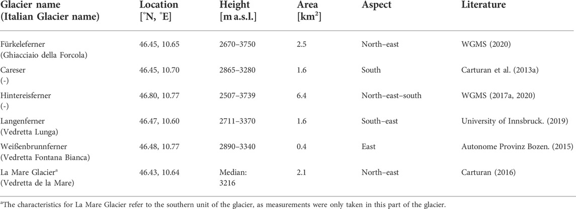
TABLE 1. Characteristics of Fürkeleferner and other glaciers in the wider study area (see comparison of mass balances of Fürkeleferner with neighboring glaciers in Section 5.3).
Glaciers with much smaller areas or southern aspects are expected to be more severely affected by climate change (D’Agata et al., 2014). This is because glaciers with a southerly orientation receive more solar radiation than glaciers with other orientations. Furthermore, small glaciers have a limited vertical extent.
The objective of this study is to investigate the current state of Fürkeleferner as a basis for understanding the glacier response to the climate during the last glacier advance of the LIA and in the 21st century. With this study we contribute to a better understanding of glacier response to past and future climate change by applying the model to a glacier representative for the region. We present simulated monthly mass and energy balances and are therefore able to analyze seasonal and annual differences in mass and energy balances. Thus, this study highlights the interplay of the energy and mass balance of glaciers with both the climatic drivers and the geometric response of the glacier and internal feedbacks as for example refreezing and albedo. This study is a step forward toward a full picture of the climate conditions during the LIA period in this region.
Fürkeleferner is a temperate valley glacier situated in the Eastern Alps (46.45° N, 10.64° E) at the head section of Martell Valley, Ortles-Cevedale massif, Northern Italy (Adler et al., 2015) (see Figure 1). Fürkeleferner has a median elevation of approximately 3,100 m a.s.l. and a glacier length of 3.5 km (WGMS, 2020). Table 1 and Figure 1 provide further details about Fürkeleferner and other glaciers in its vicinity.
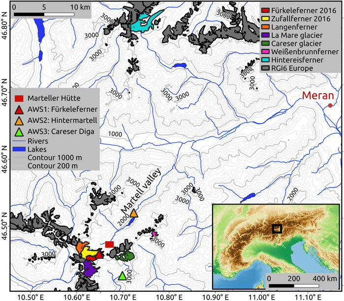
FIGURE 1. Study region Vinschgau showing Fürkeleferner and glaciers used for comparison in colors and any further glaciers in the region in dark gray. Glacier outlines are from Randolph Glacier Inventory 6.0 (RGI-Consortium, 2017). Colors in the inset map represent elevation (terrestris GmbH and Co. KG, 2021). Contour lines are derived from the Shuttle Radar Topography Mission digital elevation model post-processed data (Jarvis et al., 2008), and the surface water stem from European Environment Agency (EEA, 2020).
Most glaciers in the Ortles-Cevedale massif, Italy have a northern aspect (Carturan et al., 2013b; D’Agata et al., 2014). Fifty percent of the glaciers in the region are smaller than 0.5 km2, while 13 % of the glaciers cover an area larger than 1 km2. Mean elevations between 3,000 and 3,200 m a.s.l. are most common (D’Agata et al., 2014). Figure 2 shows a photograph from 2017 of the Fürkeleferner (left), its neighboring glacier Zufallferner (Italian glacier name: Vedretta del Cevedale; right) and the surrounding of the glaciers. During the LIA both glaciers were partly connected (see Figure 3).
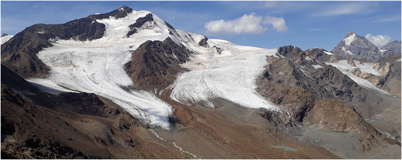
FIGURE 2. Fürkeleferner (left) and Zufallferner (middle) with middle moraine and Langenferner (right) (24 August 2017, photo by Christoph Schneider).
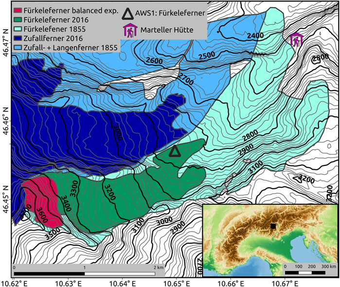
FIGURE 3. Outlines of Fürkeleferner, parts of Zufallferner, and location of the automatic weather station (AWS1) on Fürkeleferner. The outline denoted as “Fürkeleferner balanced exp.” represents the glacier area, resulting from the experiment of a present zero mass balance for current climate as described in Section 3.5.
Martell Valley is surrounded by high mountain ranges, which have a shielding effect against humidity. This makes the location one of the driest regions of the Alps (Adler et al., 2015; Galos et al., 2015; Carturan, 2016). Most annual precipitation is caused by airflow from the south mostly due to cyclonic conditions over the Mediterranean region (Galos et al., 2017). For an altitudinal range of 3,000–3,200 m a.s.l., annual precipitation is estimated to be 1,300–1,500 mm at the Careser Glacier, which is located close to Fürkeleferner, but in the adjacent catchment to the south of Fürkeleferner (Carturan et al., 2013a; Galos et al., 2017).
The mean annual 0 °C isotherm for the region is around 2,500 m a.s.l. (Carturan et al., 2013a; Galos et al., 2015). The mean annual air temperature for 2004–2013 measured at Langenferner is −3.5 °C at 3,000 m a.s.l., where July is the warmest month (+4.7 °C) and February the coldest month (−11.8 °C) (Galos and Covi, 2016).
We use the COupled Snowpack and Ice surface energy and mass balance model in PYthon (COSIPY, Sauter et al., 2020), which is based on the COupled Snowpack and Ice surface energy MAss balance model (COSIMA, Huintjes et al., 2015), to simulate glacier-wide mass balance and energy fluxes for Fürkeleferner. The source code is freely available (https://github.com/cryotools/cosipy, last access: 7 August 2021). In this study, we applied COSIPY v1.4 (http://doi.org/10.5281/zenodo.4439551, last access: 7 August 2021). COSIPY is a physically based one-dimensional model and combines the surface energy balance with a multi-layered adaptive sub-surface scheme. This type of model with physical parameterizations turns out to be a useful tool for understanding glacier mass change and its causes (Mölg and Scherer, 2012). In the distributed setup, all surface and subsurface processes are calculated at each glacier grid point. Ice dynamics, all lateral exchange between grid points and processes at the base of the glacier are neglected. Therefore, the calculated mass balance is referred to as climatic mass balance following Cogley et al. (2011). Here, we provide details on the climatic mass balance and energy balance equations solved by COSIPY. A more detailed description can be found in the work of Sauter et al. (2020).
The climatic mass balance is computed by concerning accumulation due to solid precipitation, deposition at the surface, and refreezing within the snow layers and ablation due to surface and subsurface melt and sublimation. The climatic mass balance (CMB) can be formulated as follows:
where QM is the energy available for surface melting, QE equals the turbulent latent heat flux, and csolid and cref refer to solid precipitation and refreezing of percolating water in the snowpack, respectively. Percolating water consists of surface melt and rain. A small proportion of shortwave radiation penetrates the upper layers and can result in subsurface melt amelt,sub if the layer temperature is at the melting point of water (0 °C). Latent heat of fusion LF is set to 3.34 × 10⁵ J kg−1, while 2.834 × 10⁶ J kg−1 is used as latent heat of sublimation LS (Huintjes et al., 2015; Sauter et al., 2020). If the surface temperature Ts is at the melting point of water and the energy flux F is positive, QM can occur. The energy balance equation is determined by the sum of energy fluxes:
with SWin incoming shortwave radiation, α surface albedo, LWin and LWout incoming and outgoing longwave radiations, respectively, and QH and QE turbulent sensible and latent heat fluxes, respectively. QG represents glacier heat flux and QR the sensible heat flux of rain. SWin is calculated for every grid cell using the model developed by Kumar et al. (1997). This model provides potential incoming shortwave radiation SWin,pot calculated for clear-sky conditions. A digital elevation model (DEM), geographic location, and a glacier mask serve as input variables for this approach. Following Kumar et al. (1997), altitude, shading, aspect, slope, season, and albedo are taken into account. Furthermore, the model corrects for diffuse and reflected radiation. Relief shading is not considered. To receive a corrected SWin where cloudiness is considered, SWin,pot is corrected for every grid cell using the cloud cover fraction N. Thereby, diffuse radiation during 100 % cloud cover is not taken into account. SWin is calculated as follows:
Albedo α is calculated after Oerlemans and Knap (1998) and depends on snow aging and snow depth, and constant albedo values for new snow (0.9), firn (0.55), and ice (0.2) (Oerlemans and Knap, 1998; Huintjes et al., 2015; Sauter et al., 2020). LWin is parameterized with N, air temperature, and atmospheric emissivity (Stefan–Boltzmann law). Atmospheric emissivity is parameterized with clear-sky emissivity, emissivity of clouds, and N (Klok and Oerlemans, 2002). All other terms on the right-hand side of Eq. (2) are dependent on Ts. Ts is solved iteratively with a Newton–Raphson optimization algorithm. LWout is parameterized with Ts, and surface emissivity via the Stefan–Boltzman law. A Bucket approach (Stull, 1988; Foken, 2008) is used to calculate the turbulent fluxes (QH and QE) based on the flux-gradient similarity (Prandtl, 1935; Sverdrup, 1936). The Bulk Richardson Number is used for stability correction (Stull, 1988). The surface roughness length is calculated following Mölg et al. (2012). For ice it is set to a constant value (1.7 mm), and for snow-covered areas it evolves from the surface roughness of new snow (0.24 mm) to the value of firn (4 mm) depending on time (Mölg et al., 2012). The roughness lengths for the transfer moisture and sensible heat are estimated to be one and two orders of magnitude smaller than the surface roughness (renewal theory for turbulent flow, Smeets and van den Broeke, 2008; Conway and Cullen, 2013). Energy fluxes are of positive (negative) algebraic sign toward (directed away from) the surface. Mass balance components are positive (negative) if they are a mass gain (loss).
A DEM from 2017 (Autonome Provinz Bozen, 2017) was used for topographic information of the glacier, which is important for local climatic conditions, for example, temperature, air pressure, and for the spatial distribution of solar radiation (Beniston, 2006). Model simulations were performed using the DEM with a resolution of 30 m. The glacier outline from September 2016 was obtained from a Landsat 8 satellite image (United States Geological Survey, 2016).
Meteorological variables (Table 2) are required to force COSIPY. During two summer field campaigns 2016 (15–18 August) and 2017 (21–25 August), we operated an automatic weather station (AWS) directly located on the ablation area of Fürkeleferner (hereafter AWS1). AWS1 was set up at an altitude of 2,864 m a.s.l. (2016) measuring air temperature, ice temperature, relative humidity, precipitation, wind speed, and radiation fluxes.
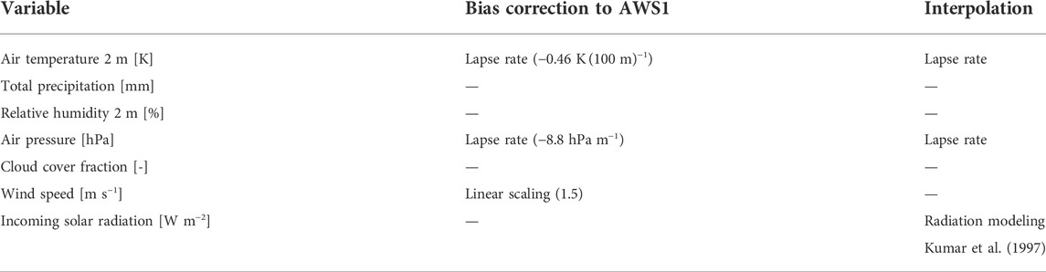
TABLE 2. COupled Snowpack and Ice surface energy and mass balance model in PYthon (COSIPY) forcing variables with required units, applied bias correction to correct data from the altitude of the automatic weather station (AWS2) to the altitude of AWS1 and approaches to create the distributed fields (interpolation) on the glacier. A dash stands for no correction.
Due to short observation periods, in situ data from AWS1 could not be used to force the model. Instead, data measured from October 2012 to September 2017 at AWS Hintermartell (AWS2) operated by the Weather and avalanche service of the Autonomous Province of Bozen (Weather and avalanche service Autonomous Province of Bozen, 2020) (46.5169° N, 10.7269° E, 1,720 m a.s.l.), which is about 9.4 km away from Fürkeleferner (Figure 1), was used to derive continuous meteorological forcing for the model (Table 2). Hereafter, we use the term mass balance year in accordance with the hydrological year starting with the approximated beginning of the accumulation season on 1 October.
The 5-year atmospheric forcing allows a trade-off between computational effort and a sufficiently long period to analyze the current state of the glacier. To ensure that the atmospheric forcing represents, on average, the climate of the first 2 decades of the 21st century, we compare temperature and precipitation of the nearest grid point of the atmospheric reanalysis ERA5 for both periods (see Supplementary Figures S1,S2). The ERA5 data for 2000–2020 and October 2012 to September 2017 are similar, which indeed justifies that the 5-year simulation period provides a good representation of the overall climate conditions of the first two decades of the 21st century in the area. Moreover, there is a reasonable agreement between the atmospheric forcing data used for glacier simulation and the ERA5 data in the same period.
From AWS2 sub-hourly meteorological data were used to calculate hourly means, respectively totals for precipitation, for all AWS2 data. For all model simulations sunshine duration from AWS2 was used to calculate cloud cover fraction N as
where SD is the sunshine duration within 10 min in seconds.
Precipitation usually increases with altitude while air temperature and absolute humidity decrease with altitude (Gerbaux et al., 2005; Beniston, 2006). Furthermore, wind speed and complexity of spatial snow distribution are higher with altitude (Carturan, 2016). Therefore, a correction of data from AWS2, located much lower than AWS1, was necessary.
For air pressure, we calculated a linear gradient of −8.8 hPa m−1 between AWS1 and the valley station AWS2. For relative humidity, no reasonable lapse rates could be obtained. Wind speed showed an underestimation of AWS2 compared to AWS1. In 2016, the mean wind speed at AWS1 was 1.9 times the mean wind speed at AWS2, and in 2017 it was 2.2 times the mean at AWS2. Therefore, we applied a scaling factor of 1.5 to the wind speed data of AWS2, which is a conservative estimate, but was chosen due to the small number of observation days at AWS1.
As already small variations in air temperature and precipitation impact mass balance (Carturan et al., 2015), we calculated lapse rates for air temperature and precipitation between AWS2 and AWS Careser Diga (hereafter AWS3). AWS3 (46.4226° N, 10.6989° E, 2,600 m a.s.l., Meteotrentino, 2020), is located about 5 km away from Fürkeleferner. Both, AWS2 and AWS3 provide data for air temperature and precipitation for the whole study period, which allows calculating reliable lapse rates. The hourly mean air temperature lapse rate is −0.46 K (100 m)−1 (r: 0.88) while the hourly mean precipitation lapse rate is 1.3 % (100 m)−1 (r: 0.36) and was therefore set to zero. The model set up using the described lapse rates is called “reference run.”
Temperature measurements from all three AWS during the short-term observation periods in 2016 and 2017 show a similar course. Temperature amplitudes are highest at the valley (AWS2). Precipitation measurements are different in time and amount. Highest precipitation is measured at AWS3, while precipitation events at AWS2 are scarcest in 2016. In 2017, precipitation is only present at AWS2. Minimum temperatures of the altitude-adjusted temperature from AWS2 to the altitude of AWS1 during those periods match well, while maximum temperatures differ to some extent. This is caused by distinct temperature amplitudes between day and night at the valley station AWS2. The altitude-adjusted data from AWS2 to the altitude of AWS1 show an annual mean air temperature of −0.7 °C and mean annual precipitation of 924 mm.
COSIPY separates total precipitation in solid and liquid using the approach after Möller et al. (2007) according to air temperature. The approaches listed in Table 2 were applied to receive meteorological distributed data over the whole glacier area from the point data of AWS2 after adjustments to compensate for the effects of altitude.
To assess the uncertainty of the glacier-wide climatic mass balance to the model parameters and the climate forcing variables, we used the package Statistical Parameter Optimization Tool for Python (Houska et al., 2015), which includes an opportunity for global sensitivity analysis based on the Fourier amplitude sensitivity test by Saltelli et al. (1999). Due to computational demand we split the experiments in three parts and had to limit the number of simulations. First, we varied 10 most sensitive model parameters by executing 1,000 simulations. Second, we varied the meteorological forcing variables with glacier-wide offsets and scaling factors (depending on the input variable) within another 1,000 simulations, and third, we varied the lapse rates of air temperature, precipitation, and relative humidity by executing 200 simulations. We had to reduce the spatial resolution from 30 to 100 m to speed up the simulations for the sensitivity experiments. The difference in the annual climatic mass balance between both simulations with 30 m and with 100 m spatial resolution is less than 0.2 m w.e.
Tested model parameters include the albedo of new snow, firn, and ice, albedo time scale, albedo depth scale, roughness new snow, firn, and ice, center temperature of the snow-to-rain transfer function, and spread of the snow-to-rain transfer function. Table 3 shows the ranges of the varied parameters and variables.
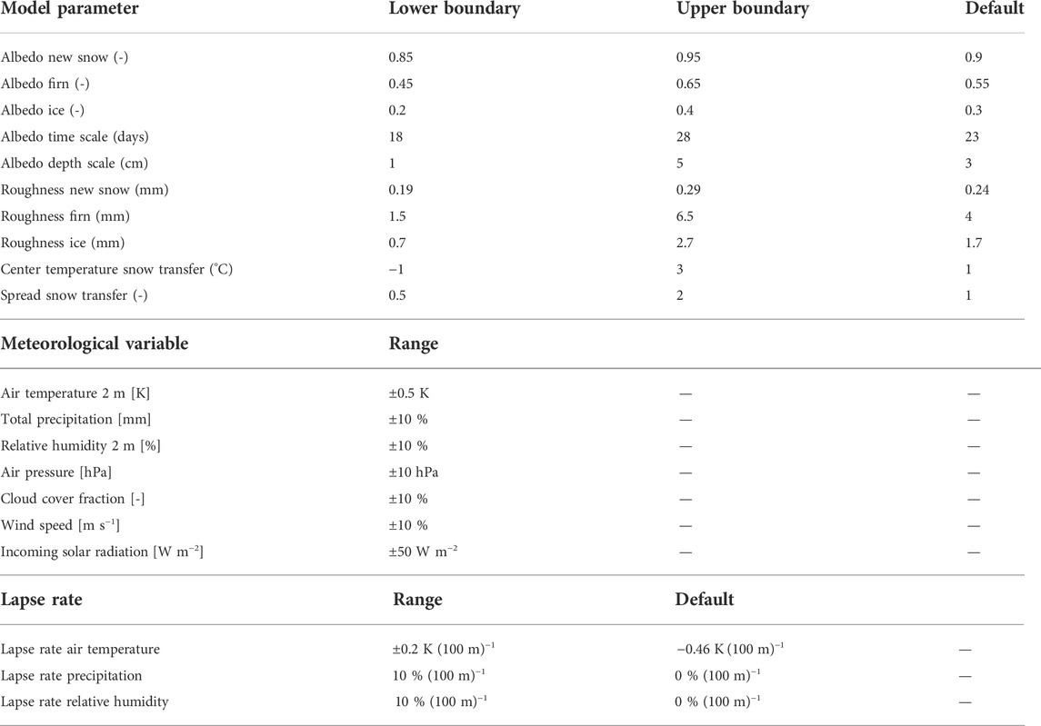
TABLE 3. Varied model parameters and meteorological forcing variables for the sensitivity experiments.
The frequency distributions of the climatic mass balances of the three experiments sorted into ranges is shown in Supplementary Figures S3–S5. The experiment with glacier-wide offsets or scaling factors, depending on the respective input variable, resulted in an annual standard deviation of 0.73 m w.e. This rather large uncertainty is a conservative estimate due to the large ranges of the perturbations for in particular temperature (±0.5 K), cloud cover (±10 %), and incoming solar radiation (±50 W m−2). The experiment regarding variable lapse rates resulted in an annual standard deviation of 0.31 m w.e. The sensitivity experiment regarding the model parameters resulted in an annual standard deviation of 0.25 m w.e. The total annual uncertainty of ±0.83 m w.e. is calculated from the root of the sum of the three squared standard deviations.
To assess the reliability of the simulations, we compare the averaged simulated and measured daily mass balance data for different altitude ranges from single day observations on Fürkeleferner in summer 2016 to 2019 and 2021. The measurement periods and number of stakes per year are presented in Supplementary Table S1. Results are shown in Figure 4. COSIPY shows less melt than the observations at ablation stakes (approximately 0.03 m per day averaged from about 20 days of observations). However, we assume that measured melt amounts are very high. The measurements were carried out by students who had no previous experience with ablation stake measurements. Therefore, the measurements were probably taken too close to the ablation stake hole and thus in the melting funnel. Furthermore, there was strong heat conduction at plastic stakes, especially in the first days after installation. This was actually the case, due to the short measurement periods. Further uncertainties were introduced by site specific features of ablation stakes, which in few cases were affected by small supraglacial melt water streams or by either smaller or higher than average ice albedo. To investigate whether COSIPY underestimates summer ablation, we calculate the annual winter mass balance assuming the overall annual mass balance is simulated correctly, and compare it with measured winter mass balances of neighboring glaciers (see Section 5.3). Unfortunately, long-term mass balance measurements from ablation stakes are not available since all stakes left behind for measuring annual mass balance in the lower part of the ablation zone had melted out until the following summer.
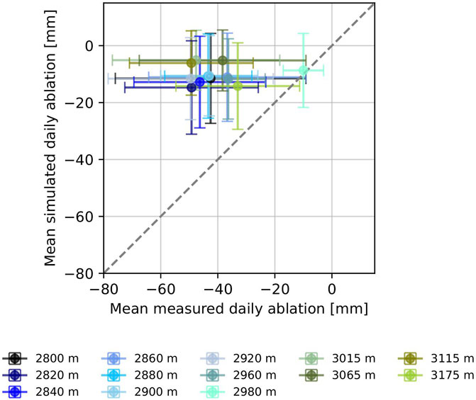
FIGURE 4. Simulated mass balance in comparison with observations at ablation stakes during consecutive days as measured during student field courses in summer 2016 to 2019 and 2021 (see Supplementary Table S1 for exact dates). Data are averaged over altitude ranges of 30 m for altitudes below 3,000 m and 50 m above 3,000 m. The standard deviation bars represent the spatial and temporal distribution of the measured and simulated mass balance each.
We assume high measurement biases due to measurements carried out as part of a student field course with these students measuring and installing ablation stakes for the first time and reading of the stakes only shortly after installation. Thus to investigate the validity of the observations, we calculated the degree-day factor (Hock, 2003; Carturan et al., 2012; Wake and Marshall, 2015) for each altitude range using the respective average air temperature of all days and the measured melt rates. Results are shown in Figure 5. The mean degree-day factor of 6.1±1.4 mm day−1 °C−1 is higher than degree-day factors reported in other studies for the region. Carturan et al. (2012) used a degree-day factor of 3.84 mm day−1 °C−1 for the neighboring glaciers Careser and La Mare. Bombelli et al. (2019) used a degree-day factor of 5.13 mm day−1 °C−1 for the Italian Alps. In conclusion, the degree-day factor obtained from summertime measurements on Fürkeleferner is higher than the degree-day factors reported elsewhere for the region. This backs our assumption that the observations may overestimate real melt rates. Therefore, these can only be used as an indication and for a rough comparison with simulations. In any case, observations and simulations clearly show high melt rates during the respective measurement periods.
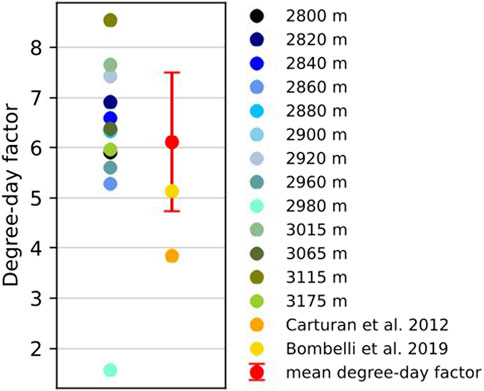
FIGURE 5. Degree-day factors for glacier Fürkeleferner averaged over the measurement periods presented in Supplementary Table S1 . Data are averaged over altitude ranges of 30 m for altitudes below 3,000 m and 50 m above 3,000 m. Furthermore, the mean degree-day factor and standard deviation and values from Carturan et al. (2012) and Bombelli et al. (2019) are presented.
To further validate the simulated mass balance results, we compared simulated mass balances with estimated geodetic mass balances by Davaze et al. (2020) between 2013 and 2016. The geodetic mass balances in Davaze et al. (2020) are only available for the joint area of Fürkeleferner and Zufallferner, since they are defined as one glacier in the Randolph Glacier Inventory 6.0 (RGI-Consortium, 2017). Zufallferner has large areas at high altitudes, resulting in less negative annual mass balance than if only Fürkeleferner is considered. Furthermore, both the annual geodetic data and the COSIPY runs include large ranges of uncertainty. Therefore, we only compare relative interannual variability. While simulated mass balance in 2014 (−1,203 mm w.e.) is considerably more negative than 2013; Davaze et al. (2020) found only slightly negative mass balances (‒220 mm w.e.) for both years. This underpins that the simulated mass balance in 2013 might be too negative. As we have not applied any spin-up time for the simulations, the time COSIPY needs to adjust to the surrounding boundary conditions possibly influences this result. The relative interannual variability of 2014, 2015, and 2016 is similar in both datasets with only slightly negative mass balances in 2014 and more negative mass balance in 2015 and 2016 with −1,669 mm w.e. (2015) and −1,883 mm w.e. (2016) simulated for Fürkeleferner, and −840 mm w.e. (2015 and 2016) derived by Davaze et al. (2020) for the joint area of Fürkeleferner and Zufallferner.
To assess the reliability of the results, we further compared measured mass balances of neighboring glaciers in the European Alps (Table 1), in particular in the Ortles-Cevedale massif, with the simulated mass balances of Fürkeleferner (see Section 5.3). Direct glaciological measurements provided annual mass balances for Langenferner (Autonome Provinz Bozen, 2015; Galos et al., 2017; University of Innsbruck, 2019), Careser (WGMS, 2017b), Hintereisferner (WGMS, 2017a), La Mare (Carturan, 2016), and Weißenbrunnferner (Autonome Provinz Bozen, 2015).
To study glacier sensitivity to temperature change, temperature was increased by +1 K and +2 K concerning the expected temperature rise for the European Alps in the 21st century (Heinrich et al., 2013) instead of using projected future climate forcing data. The influence of other forcing variables, which also may change in the future (e.g. precipitation, wind, cloud cover, and moisture), and the changing glacier hypsometry were not considered, although they are all complexly linked with each other. Lapse rates were maintained as in the reference run. A similar approach was also used by Gerbaux et al. (2005) and Möller et al. (2007). No seasonal variations were taken into account.
We then evaluated changes in climatic mass balance with altitude for an increase in air temperature of +1 K and +2 K in comparison to the present climate. In addition, we investigated differences in energy and mass fluxes for the present climate and a +2 K warmer climate to analyze the reasons for differences in the climatic mass balance. Glacier areas commonly decrease in the European Alps even without any additional temperature increase to reach steady state conditions, resulting in a projected glacier area decrease of about 50 % in the Ortles-Cevedale group (Carturan et al., 2013b; Galos et al., 2015; Smiraglia et al., 2015). Thus, to investigate if Fürkeleferner could remain under present climatic conditions with a smaller glacier area (see Figure 3 for outline), we studied the potential glacier climatic mass balance under present climatic conditions for a largely reduced glacier area.
To investigate temperature and precipitation differences between 1855 and today, the glacier was set in equilibrium by varying the forcing data of temperature and precipitation until the simulations resulted in a zero mass balance. For this experiment, we use the glacier outline from 1855 and an estimate of the glacier surface following similar approaches as Huintjes et al. (2016) and Weidemann et al. (2020). All other model settings were left unchanged.
To determine the glaciers’ past outlines, we used terrain structures, for example, lateral and terminal moraines visible in the DEM and aerial photographs (Microsoft, 2021). The results were compared with the findings of Müller (2006) who dated moraines in the wider study area, the Hinteres Martell Valley. For Fürkeleferner and Zufallferner, Müller (2006) found moraines from 1680, 1820, 1855, 1895, and 1920. Moraines that Müller (2006) dated to 1855 were used to support the reconstruction of the glacier extent of Zufallferner and Fürkeleferner for the last LIA maximum. Further reconstructions of LIA extents for South Tyrol are conducted for La Mare Glacier by Carturan et al. (2014), for the Rieserferner Group by Damm (1998), for Trentino by Zanoner et al. (2017), and for the Italian Autonomous Province of Bozen by Knoll et al. (2009). The reconstructed glacier outline from 1855 worked out from Müller (2006) corresponds with the findings from our field survey, during which we mapped the moraines between Fürkeleferner and Marteller Hütte, and also with the analyses of aerial photographs and the DEM, which we used as a basis for reconstructing the glacier outlines of Fürkeleferner and Zufallferner during the last LIA maximum.
We first used the same forcing and DEM as for the other simulations but the past glacier outline as reference simulation to investigate past mass balance. However, during 1855 the glacier surface was at a higher altitude than today due to a larger ice volume. Therefore, we adapted the present DEM to match presumably existing past conditions as of 1855 as was also performed for other studies (Carturan et al., 2019). By using the DEM from today and an adapted DEM for the time of the LIA we can estimate the effects of terrain elevation changes on the climatic mass balance.
To use a reference to how the glacier surface might have looked like in the past, we have developed the following approach for this manuscript to adapt the current DEM to 1855 conditions. The curvature of the glacier is presumed to be similar in the past and in the present. We can hence calculate a curvature factor b perpendicular to the flowline as
where wt0 is the present distance between left and right glacier margins, wt1 is the past distance between left and right glacier margins, ht0 is the present height difference between mean margin and flowline, and ht1 is the past height difference between mean margin and flowline. The curvature factor is used to calculate the altitude of the grid point amt1 along the past flowline by
where alt1 and art1 are the past altitude of the left and the right glacier margins, respectively. The same method was similarly used to calculate the altitude for additional grid points.
Particularly in the ablation area, glaciers usually have their highest elevation in the middle of the glacier. Since there are areas where Fürkeleferner and Zufallferner formed one glacier during the LIA (Figure 3), the maximum height presumably was approximately in the middle of the area that both glaciers together formed. Therefore, for this region, the horizontal extent of both glaciers was taken into account for the calculations of the curvature factor, the altitude of the grid point along the past center and additional points.
In the area where there is currently no glacier, existing nunataks on both sides of the LIA glacier area and parts of the former middle moraine between Fürkeleferner and Zufallferner served as reliable reference points for the former glacier height. In addition, bedrock formed the glacier margin on the right side of the glacier and presumably did not change in height so that the latter can also be used as reference height. The present-day heights of the lower glacier margin were taken as additional reference points, as we assume that the lower glacier margin had approximately the same elevation as the present-day terrain. Furthermore, terrain and vegetation observations in the field helped us to estimate ice-free areas during the LIA as well as the probable flow direction and gradient of the glacier. All new grid points with a lower altitude than the present DEM were set to the present DEM altitude as the past glacier surface presumably was not any lower than the present surface.
Using ARC GIS 10.7.1, a spline interpolation resulting in the typical curved glacier shape was used to interpolate a full 1855 glacier DEM with a resolution of 30 m from the point data created in the previous step (ESRI, 2020). Finally, the DEM of the past glacier area was embedded in the surroundings of the current DEM to ensure that no extreme values occur at the edges of the DEM due to the interpolation of supporting points exclusively within the glacier area.
Figure 6 shows simulated monthly mean energy and mass fluxes for the mass balance years 2013–2017, while Table 4 presents the average annual energy fluxes. The main energy source is QSWnet (22.4 W m−2). QSWnet shows a clear course over the year with maximum in summer. QM (−20.0 W m−2), which describes the energy surplus available for melting when Ts is at the melting point, is associated with high positive QSWnet. Melting (QM < 0) occurs on average from May to September. During the study period, QM is lowest in 2014 (−9.4 W m−2), implying less ablation than in other years. Highest ablation is simulated for 2017 (−25.1 W m−2). QH, as energy source, and QLWnet and QE, as energy sinks, have similar absolute numbers ranging from −4.1 to +5.3 W m−2. The remaining fluxes QG and QR contribute only marginally to the energy balance.
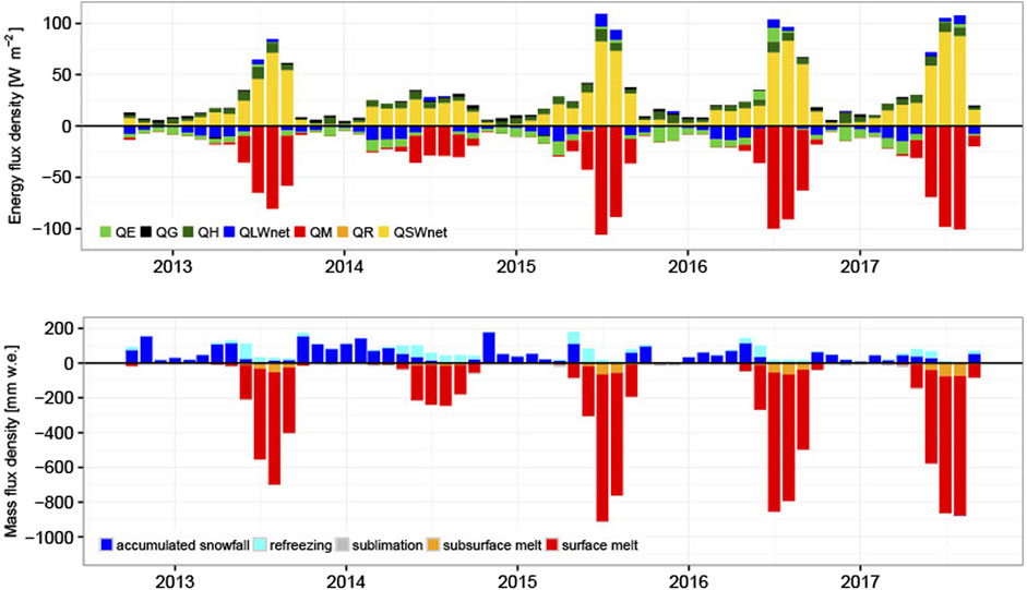
FIGURE 6. Monthly density fluxes October 2012–September 2017. Top: energy. Bottom: mass. QLWnet: longwave radiation, QE: turbulent latent heat flux, QR: heat flux from rain, QSWnet: shortwave radiation, QG: glacier heat flux, QM: energy available for surface melting, and QH: turbulent sensible heat flux.
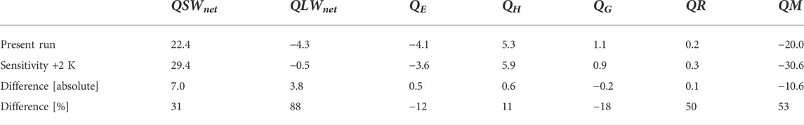
TABLE 4. Average glacier-wide energy fluxes [W m−2], 2013–2017.
Observed ice albedo during the field periods at AWS1 ranges from 0.34 to 0.40 (2016) and from 0.23 to 0.30 (2017), with no snow present at AWS1. COSIPY simulates an ice albedo of 0.3 for these periods, which is the constant set for bare ice. This seems to be a good approximation as the observed values for bare glacier ice are slightly below and above 0.3 (see Supplementary Figure S6).
As shown in Figure 6 and Table 5, accumulated snowfall (580 mm w.e.) is the main source of mass gain and contributes mostly in spring and autumn, while refreezing (195 mm w.e.) is important in summer. Surface melt (−1,906 mm w.e.) is the main driver of ablation and more than 2.4 times higher than total accumulation. Subsurface melt contributes to a small extent mainly between July and September, while about 10 % of yearly snowfall sublimates (Table 5).
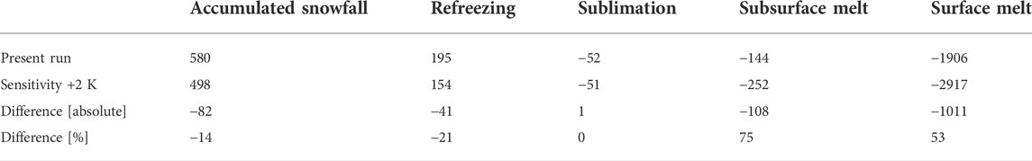
TABLE 5. Mean glacier-wide annual mass fluxes [mm w.e.], 2013–2017.
Simulated annual mean climatic mass balance from 2013 to 2017 for Fürkeleferner is clearly negative with −1,384±833 mm w.e. (see Section 3.3 for details on the uncertainty estimate). Table 6 presents simulated annual climatic mass balance for every mass balance year for Fürkeleferner. The glacier climatic mass balance shows a clear dependency with altitude (Figure 7). Maximum annual climatic mass balance for 2013–2017 shows a small accumulation area with mass gain of up to 503 mm w.e. However, annual climatic mass balance for major parts of the glacier is considerably negative with up to −3,021 mm w.e. in the lowest parts of the glacier.
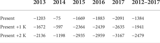
TABLE 6. Simulated mean annual glacier-wide climatic mass balance [mm w.e.] of Fürkeleferner from 2013 to 2017.
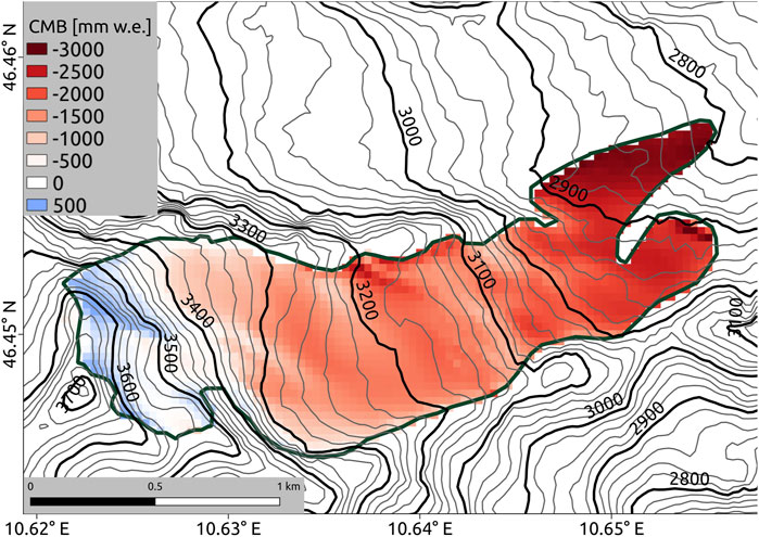
FIGURE 7. Spatially resolved simulated mean annual climatic mass balance (CMB), 2013–2017 [mm w.e.] for present climate.
Investigating single year accumulation areas (see Supplementary Figure S7), simulations only show a pronounced accumulation area for 2014. The mass balance years 2013 and 2015 show high annual mass losses, combined with only slightly positive mass balance for small areas in the uppermost part of the glacier. Moreover, during mass balance years 2016 and 2017 no accumulation areas were found but negative mass balances prevail throughout the whole glacier area. In general, the ablation area and ablation clearly exceed accumulation area and accumulation which is reflected in the considerably negative mean annual climatic mass balance of −1,384±833 mm w.e. Therefore, under meteorological conditions similar to those prevailing during the study period, the glacier loses mass over most of its area with only small areas of accumulation during some years.
For current climatic conditions we are able to simulate a zero climatic mass balance for a considerably reduced glacier area of 0.29 km2, 17 % of today’s area of Fürkeleferner (see “Fürkeleferner balanced exp.” in Figure 3). This indicates that Fürkeleferner would have to heavily reduce its area to a small cirque glacier in regions above 3,400 m a.s.l. to be under steady state conditions with the current climate.
To investigate the glacier sensitivity to increasing air temperature we increased present air temperature by +1 K and +2 K. This largely impacts mean annual mass balance of Fürkeleferner. Figure 8 shows the mean annual mass balance gradient for today’s temperature and increased temperature by +1 K and +2 K. Mass balance for simulations with higher air temperature become considerably more negative over the entire glacier than for the reference run. Cumulative mass balance is 1.4 times (+1 K) and 1.8 times (+2 K) more negative than for present air temperature. Furthermore, results in Figure 8 clearly show that there is no accumulation area left under such scenarios. This means that the glacier would eventually melt entirely in the future under scenarios with higher air temperature.
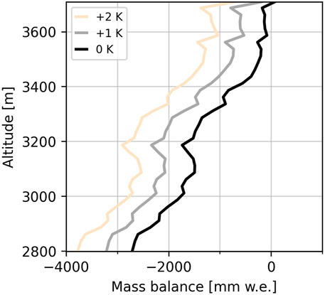
FIGURE 8. Sensitivity of the mean annual mass balance gradient [mm w.e.] to temperature changes.
We compare energy- and mass fluxes (Tables 4, 5) of the reference run with results for a temperature increase of +2 K as projected for the European Alps even under moderate climate scenarios (Heinrich et al., 2013; Gobiet et al., 2014) to attribute enhanced ablation to driving mechanisms. An increase of 31 % in QSWnet and a decrease in QLWnet of 88 % leads to an enhanced QM of 53 %. Enhanced air temperature causes less snowfall (−14 %) and refreezing (−21 %), triggering positive energy fluxes and generally leads to longer ablation seasons with more melting. Concerning a temperature increase of +2 K differences in solid precipitation, surface (53 %) and subsurface (75 %) ablation in comparison with the reference run are the main drivers for enhanced ablation for Fürkeleferner. The significant difference in ablation is caused by decreasing the snow cover, which results in lower albedo. Therefore, SWout is lower than for the reference run and SWnet is enhanced.
Figure 9 shows the difference between the present DEM and the altitude-adjusted DEM for the extent of the maximum of the last LIA glacier advance. Main differences (up to 300 m) in the DEMs are visible in the today ice free zone, the former ablation area of the glacier.
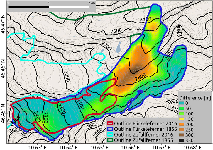
FIGURE 9. Calculated height differences between the digital elevation model (DEM) adapted to Little Ice Age (LIA) conditions during the maximum of the last LIA glacier advance and the DEM from 2011 (Autonome Provinz Bozen, 2011).
Based on the results of the moraine mapping we conducted in the field and the comparison with glacier outlines from Müller (2006) for 1855, we derive a glacier area of about 4.69 km2 for 1855, which is about 2.8 times larger than during the study period (2013–2017). For the simulation with the altitude-adjusted DEM using the same atmospheric forcing as for the present simulation (2013–2017) but glacier extent from 1855 (Figure 9), we found a zero mass balance for air temperatures −3 K lower than today. For a slightly wetter climate (10 %–20 %), we found a temperature adjustment of −2.5 K visualized in Figure 10. Figure 10 also shows further possible combinations of precipitation and temperature changes compared to present climate to force the model simulation to a zero mass balance for the glacier area of 1855. Each pair of boxes shows the temperature and precipitation perturbation required to achieve near steady state conditions with a mass balance close to zero. For example, a 1.5 K colder climate during the LIA and a precipitation change of 60 % yields a slightly negative mass balance of −0.33 m w.e. The same −1.5 K temperature change and a precipitation change of 70 % yields a positive mass balance of +0.26 m w.e.
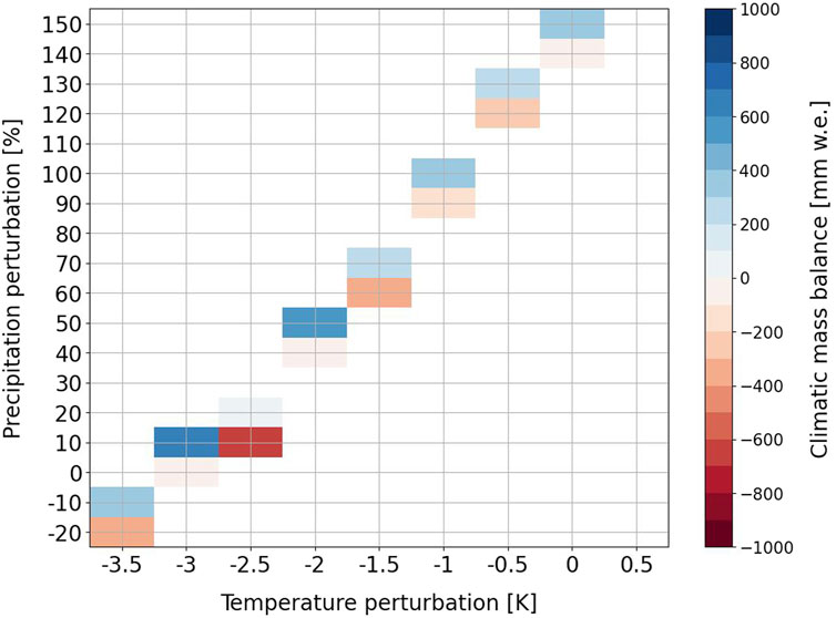
FIGURE 10. Precipitation and air temperature offsets to simulate a zero glacier-wide cumulative mass balance [mm w.e.] for the LIA extent during the maximum of the last LIA glacier advance of Fürkeleferner based on the adapted digital elevation model. The colors denote the simulated glacier-wide mass balance [mm w.e.], 2013–2017. We consider any increase of precipitation above 40 % as unrealistic. Thus, these values are only for the purpose of demonstrating the principally possible combinations.
Thereby, the higher the precipitation the less cooling is necessary compared to current climate to achieve approximate steady state conditions. However, as visible in Figure 10 the relationship between temperature change and precipitation change to receive a zero climatic mass balance is not linear. For cooling of −3.5 K or more, even a decrease in precipitation may lead to steady state conditions. To reach nearly steady state conditions without any decrease in temperatures, precipitation would have to rise by +140 to +150 %. Forcing the model with current climatic conditions, but with the glacier extent from 1855, results in a strongly negative annual mass balance using the present DEM of ‒2,054 mm w.e. and ‒1,844 mm w.e. for the altitude-adjusted DEM for the extent of the maximum of the last LIA glacier advance.
Meteorological data from AWS2 adjusted with linear gradients to the altitude of AWS1 on the glacier are a major source of uncertainty due to changing lapse rates over time, more complex relationships, and local influences. Mountain shading effects can further influence the meteorological input parameters (Gerbaux et al., 2005). Several studies showed that applying linear lapse rates to meteorological data, for example to extrapolate air temperature should be used with caution (Carturan et al., 2015). The microclimate at Fürkeleferner can be very different compared to the microclimate measured at the surrounding AWS. Discrepancies can be caused by temperature inversions, valley, or glacier winds (Beniston, 2006).
Precipitation, even at the scale of a mountain range, is highly variable and very local among others due to topographic effects. AWS1 and AWS2 are located on the northern side of the Ortles-Cevedale massif, and AWS3 on the southern side of the massif. This can lead to systematic differences, especially in precipitation. The Cevedale mountain ridge (German: Zufallspitze) is a meteorological divide. More precipitation falls south of the ridge than north of the ridge, which means that the Martell Valley (AWS1 and AWS2) is in an intra-montane dry zone (Golzio et al., 2018). Therefore, precipitation at AWS3 might be higher than at Fürkeleferner AWS1, and the calculated lapse rates between AWS2 and AWS3 might not be representative for the lapse rate between AWS1 and AWS2. However, during southern inflow, orographically induced enhancement of precipitation may reach over the mountain ridge, reaching the accumulation area of Fürkeleferner.
The differences in precipitation regime are also hinted at by poor precipitation correlation (R2: 0.36) between AWS2 and AWS3. In addition, there is a clear precipitation increase with altitude around the study region, which is not considered in the model forcing data (Beniston, 2006; Golzio et al., 2018). Therefore, using the same precipitation rates for Fürkeleferner as measured in the valley at AWS2 may result in too low precipitation at AWS1. However, during the short measurement periods in the summers of 2016 and 2017, the amount of precipitation at AWS1 was in the same range as at AWS2 and AWS3. This confirms the assumption of a small precipitation lapse rate at least for the field measurements. Furthermore, precipitation lapse rate between AWS2 and AWS3 based on hourly data does not show any seasonal variation over the study period. Thus, using a constant lapse rate is appropriate.
Another source of uncertainties is the measurement of precipitation itself since wind and evaporation can lead to an underestimation of precipitation (Rodda and Dixon, 2012; Grossi et al., 2017). However, the errors are generally higher for solid precipitation than for liquid precipitation and largest at windy sites (above 50 %) (Rodda and Dixon, 2012; Grossi et al., 2017). Since we use measurements from AWS2 in the valley, snowfall is less frequent. As described before, the wind speed is lower at AWS2 than at AWS1. Therefore, we assume a small undercatch, but biases may still exist.
Air temperature is a key variable for simulating glacier mass balance caused by strong effects on the occurrence of solid precipitation, snow density, and the energy balance due to effects on turbulent fluxes and longwave radiation (Haeberli et al., 2007; Carturan et al., 2015). This can be clearly seen in the obtained results for energy and mass fluxes for increased temperature of +2 K (Tables 4, 5). Worth mentioning are especially the QLWnet, QR, and QM change ≥50 % in the energy balance and the subsurface melt and surface melt change in the mass balance (
Hourly air temperatures from AWS2 and AWS3 show a high correlation (R2: 0.88), indicating that the application of a linear lapse rate results in a reasonable approximation of air temperature over the study area despite seasonal variation in the temperature lapse rate. In addition, we suspect that errors we might introduce by using seasonally varying lapse rates between AWS2 and AWS3 to calculate temperature at the location of AWS1 to be larger than using a constant lapse rate throughout. The temperature lapse rate of −0.46 K (100 m)−1 used in this study is lower than temperature gradients reported for other glaciers from Table 1 ranging from 0.57 to 0.83 K (100 m)−1 (Carturan et al., 2015; Department of Atmospheric and Cryospheric Sciences, University of Innsbruck, 2015; Giaccone et al., 2015; Galos and Covi, 2016), which in turn could lead to an overestimation of air temperatures.
We find a distinct annual cycle in monthly calculated air temperature lapse rates. The lapse rate is lower in winter due to a higher occurrence of temperature inversions, while more convective conditions cause higher lapse rates in summer. Another reason for seasonally different temperature lapse rates may be cooling of the air caused by melting of the glacier surface and glacier wind during the ablation period (Zhou et al., 2010). During the summertime observation periods (about 1 week each in August 2016 and 2017), there are clear derivations between measured and altitude-corrected air temperature. While minimum temperatures are in good agreement, maximum temperatures are overestimated due to a higher diurnal amplitude of air temperatures at AWS2 compared to AWS1.
SWin was not measured directly but has been calculated according to Kumar et al. (1997). The parameterization of SWin as well as using cloud cover data from AWS2 to consider daily cloud coverage can introduce uncertainties. However, simulated albedo matches well with measured albedo during the observation period at AWS1.
For a combined uncertainty resulting from the input data, we conducted two experiments (see Section 3.3 for details on the uncertainty estimate), which resulted in an annual standard deviation of 0.73 m w.e. for glacier-wide offsets and scaling factors (depending on the input variable) and an annual standard deviation of 0.31 m w.e. for variable lapse rates.
To show that the selected study period of 5 years is representative of the climate in the region, we use ERA5. ERA5 has a horizontal resolution of approximately 30 km. It is able to represent the main mesoscale precipitation patterns, including differences between mountain areas and lowlands as well as between luv and lee sides. However, biases exist e.g., due to the resolution being too coarse to resolve small-scale topography (Bandhauer et al., 2022). In terms of air temperatures, ERA5 is capable of representing air temperatures in the lowlands but shows some weakness in representing temperature at higher altitudes (
COSIPY is a point model that can be run distributed over the glacier area. It resolves the climatic mass balance at each glacier grid point without any lateral energy and mass exchange on an hourly resolution. The model does not consider ice dynamics and mass gain due to snow that is redistributed from ice-free surroundings toward the glacier by strong winds and avalanches. Snow redistribution can have considerable impacts, especially on mass balance distribution over the glacier and as a source of additional mass from surrounding terrain (Dadic et al., 2010; Lüers and Bareiss, 2013; Huintjes et al., 2015; Carturan, 2016; Carturan et al., 2016). However, snowdrift can not only lead to mass gain but also can have the opposite effects in the form of mass loss due to divergence and direct sublimation of drifting and falling snow. Furthermore, snowdrift changes the water vapor gradient near the surface. In general, COSIPY is based on parameterizations, which are generalizations of more complex processes. These parameterizations depend on constants, which are taken from the literature or other studies. The combined uncertainty experiment of selected model parameters is estimated to have an annual standard deviation of 0.25 m w.e. (see Section 3.3 for details on the uncertainty estimate).
The albedo parameterization is crucial in COSIPY and similar models (Oerlemans and Knap, 1998; Mölg et al., 2012). Glacier ice albedo change depends on the surface type. The color of the ice surface and its roughness are two major controlling factors for surface albedo (Lhermitte et al., 2014; Azzoni et al., 2016). Dirty ice has a lower albedo than whitish ice (Azzoni et al., 2016). However, the model only considers one value for ice albedo (0.3). During the field studies, albedo of Fürkeleferner was considerably variable over the glacier surface due to small remnants of snow fields, roughness, and debris cover. However, the set albedo overall matches well with measured albedo during the field studies and suggests to be an appropriate approximation within COSIPY.
We run the model without using any measurements to optimize the model for the location of Fürkeleferner. However, as confirmed by the comparison of the simulated climatic mass balance for Fürkeleferner with the climatic mass balance of other glaciers of the wider study area (Figure 11), COSIPY is able to simulate a realistic climatic mass balance. This is in agreement with studies using COSIPY in other regions of the world (Sauter et al., 2020; Thiel et al., 2020; Arndt et al., 2021).
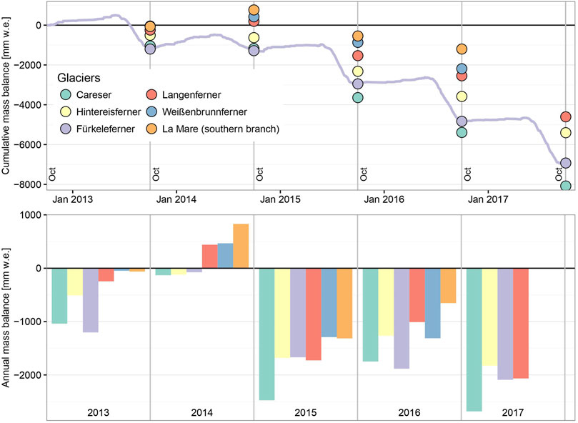
FIGURE 11. Mass balance from different glaciers, 2013–2017 [mm w.e.], of the wider study area. Top: time series of cumulative mass balance. January and October are denoted on the plot. Bottom: bar plot of specific annual mass balance without temporal evolution on the x-axis.
Net shortwave, net longwave, and turbulent fluxes are crucial for the surface energy balance of most glaciers (Weidemann et al., 2018). SWnet is controlled by atmospheric composition, cloud cover, and local topography. Surface albedo is another factor controlling SWnet (Zhou et al., 2010; Huintjes et al., 2016). Snow coverage in winter leads to higher albedo than in summer when there is mainly bare ice (Mölg et al., 2012). LWin is controlled by air temperature, humidity and cloud cover (Zhou et al., 2010). Caused by seasonal changes of these parameters LWin is highest in summer while LWout is controlled by surface temperature only and has an upper limit related to the melting point of water (Weidemann et al., 2018).
QE is smaller during summer than in winter. This is caused by lower humidity in winter, which results in a stronger (more negative) vapor pressure gradient directed away from the surface (Huintjes, 2014). In some of the summer months QE changes its sign from minus to plus. This happens when air temperature at 2 m above ground is above 0 °C and relative humidity is high. The vapor pressure gradient is directed downward and energy is released at the surface by either condensation or deposition in such cases. Overall, modeled energy fluxes show realistic and reasonable patterns.
As shown in Figure 11, both the cumulative and annual simulated mass balances of Fürkeleferner and its trend are in good agreement with those of neighboring glaciers. All glaciers in the wider area show negative mass balances during 2013–2017.
In 2013, the simulated mass balance of Fürkeleferner is most negative compared to the other glaciers possibly due to missing spin-up time to allow the model to adjust to the modeling boundary conditions (see Section 3.4). Simulated mass balance for 2014 of Fürkeleferner is almost in equilibrium, while some other glaciers show a small mass gain (Langenferner, which is closest to Fürkeleferner (<2 km): +441 mm w.e (Autonome Provinz Bozen, 2015)). The year 2014 stands out in regards to simulated climatic mass balance for Fürkeleferner. We identify lower temperatures in the summer of 2014 and more snowfall in the meteorological data used to force the model as reasons for this outstandingly positive mass balance. Clearly less surface and subsurface melt occur in 2014, which causes less melting for Fürkeleferner compared to other years in the study period. In addition, there is more solid precipitation in 2014 than in the other years, which causes more mass gain. Furthermore, SWin is smaller in July and August compared to the rest of the study period, and QM is lower than in the other years. Our findings agree well with Carturan (2016) and Galos et al. (2015) who as well found higher accumulation during 2014 and a shorter ablation season, resulting in higher annual mass balances at La Mare Glacier and Langenferner than in other years. Also, for other glaciers in the wider study area mass balances for 2014 are clearly more positive in comparison to the other years of the study period (Figure 11). Mass balances in the following years are more negative for all glaciers, which can be explained in the case of Fürkeleferner by higher surface and subsurface melt caused by enhanced SWnet.
Mass balances of the considered glaciers (Table 1) vary due to different altitude ranges and spatially different meteorological parameters such as precipitation. As an example, mass balance of Careser is clearly more negative than mass balance of Fürkeleferner. The maximum altitude of Careser is about 500 m lower than the maximum altitude of Fürkeleferner, probably causing higher air temperatures at the top of Careser than at Fürkeleferner. This leads to less frequent snowfall, which might cause lower accumulation at Careser than at Fürkeleferner. In addition, Careser has a southern aspect while Fürkeleferner is exposed to northeast (Table 1). The good consistency of mass balance between all glaciers confirms a generally realistic simulation of mass balance for Fürkeleferner.
The comparison with measured winter mass balances from other glaciers in the region (see Supplementary Table S2) indicates that COSIPY systematically underestimates winter accumulation to some extent. Since annual mass balances at the regional scale are well reproduced for Fürkeleferenr using COSIPY (Figure 11), this points to an underestimation of summer ablation, partly explaining the differences between measured and simulated ablation at the ablation stakes (see Section 3.4).
Simulated mass balance for Fürkeleferner and its distribution over the glacier suggests that the glacier has only a small accumulation area, which may diminish in some years. The small accumulation area in 2014 caused by lower temperatures in summer and more snowfall is mainly responsible for the calculated zero climatic mass balance for a small cirque glacier under current climatic conditions. During the other years of the study period, only small patches of accumulation or even a negative mass balance over the entire glacier is present. This agrees well with visual observations during the field periods (Figure 2). As temperatures increase and the equilibrium line shifts to higher elevations, the equilibrium line can exceed the maximum elevation of particularly small glaciers, making them specifically vulnerable to increasing temperatures (D’Agata et al., 2014). In line with our findings, Galos et al. (2017) and Carturan et al. (2013a) identified no existing accumulation area for Langenferner and Careser for most years, respectively. On the project website1 of Galos et al. (2017), they report accumulation area ratios of 50 %, 78 %, 2 %, 11 %, and 2 % for the years 2013–2017, respectively, for Langenferner. In the years 2015, 2016, and 2017, the equilibrium-line altitude fell above the maximum elevation of Langenferner. In addition, Carturan et al. (2016) found almost no existing accumulation areas for many other glaciers in the Italian Alps for most of the years from 2004 to 2013 and concluded that the extinction of the glaciers may occur even without any further warming.
A temperature increase of +1 K or rather +2 K has significant effects on the glacier mass balance of Fürkeleferner (Table 6). Studies show that increasing mean annual air temperature has a higher impact on ablation rates than changed precipitation in the European Alps (Giaccone et al., 2015). Increasing summer melting was the main driver for negative surface mass balances in the European Alps in the last 30 years (Vincent et al., 2017). Also Gerbaux et al. (2005) and Haeberli et al. (2007) found that precipitation is of minor importance for long-term mass balance trends. Therefore, we assume that uncertainties introduced by maintaining all variables constant but air temperature are small for assessing the overall future trend, resulting from future climate change. The presented warming experiment may serve as an initial estimate for a possible future trend.
However, melting of the glacier also leads to a reduction in ice thickness and thus terrain height. We have not considered changes in glacier hypsometry in the future climate simulations. The lack of melt-elevation feedback could result in an even smaller area for a zero climatic mass balance than in the results presented in this study. However, the upper part of the glacier rests on the steep walls of the cirque below the summit of Zufallspitze. It therefore is probably relatively thin so that adjustments in glacier hypsometry are expected to be small.
We compared the general direction of the results to the results of Zekollari et al. (2019) who used an ice dynamic model for simulations for the entire European Alps. A direct comparison however is difficult as their results include a gross of different glaciers, for example, type, size, exposition, and altitude. While we found a reduction of the glacier area of 83 % to be in the steady state with the climate of 2013–2017; Zekollari et al. (2019) found a reduction of 90 % in volume for small glaciers located in low altitudes and in general of 35 % of volume and area for the entire Alps when forced with the mean 1988—2017 surface mass balance without additional warming until 2100.
Furthermore, Zekollari et al. (2019) found glacier area losses for the entire European Alps of 62.1±8.4 % under the United Nations (UN) Intergovernmental Panel of Climate Change (IPCC) Representative Concentration Pathway (RCP) 2.6 scenario, corresponding to a global air temperature increase of 0.3 K–1.7 K until 2100 (IPCC, 2014) and of −74.9±8.3 % under the RCP4.5 scenario, corresponding to a global air temperature increase of 1.1 K–2.6 K until 2100 (IPCC, 2014). However, most glaciers located at low altitudes already disappear under the RCP2.6 scenario until 2100 (Zekollari et al., 2019). This is, in such general terms, in good agreement with the results from applying COSIPY to Fürkeleferner in this study.
Gerbaux et al. (2005) reported a higher sensitivity of the glacier ablation area than the accumulation area to meteorological changes. This seems to be connected with albedo feedbacks (Galos et al., 2015). For Fürkeleferner no different effects of increasing air temperature for different altitude ranges can be determined (Figure 8). We suspect the small accumulation area of Fürkeleferner being left only in some years under current climatic conditions as indicated by the simulations to be the reason for that. As a result, the simulated area consists mainly of the ablation area. This is the area of the glacier that is most heavily affected by increasing air temperatures due to the albedo feedback as the exposed glacier ice has a lower albedo than the snow in the accumulation area (Gerbaux et al., 2005). We show that for a considerably smaller glacier area for Fürkeleferner a zero climatic mass balance can be simulated for current climate conditions. However, even moderate climate scenarios project an increase of +2 K for the European Alps (Gobiet et al., 2014). Therefore, we conclude that it is possible that Fürkeleferner will melt down completely within probably only decades. However, for a more accurate projection, other factors such as change in glacier hypsometry and the ice-dynamical response should also be taken into account.
We use moraine mapping for the glacier outline and an altitude-adjusted DEM for the glacier surface of 1855 to reproduce the altitude conditions prevailing at the time of the maximum during the last LIA glacier advance, as the present DEM cannot correctly represent those past conditions (Carturan et al., 2013b, 2019). Based on the old middle moraine between Fürkeleferner and Zufallferner in the today ice-free part from about 2,600 to 2,800 m (see Figure 3), the glacier surface in 1855 at this moraine had to be at least 100 m higher than today in order to be able to form this middle moraine due to greater glacier thickness. Furthermore, the middle moraine was probably higher in 1855 than it is observed today due to erosion and subsidence after the melting of the ice. With the approach to adjust the altitude of the DEM to past conditions, we obtain higher altitudes of Fürkeleferner, especially in the region of the old middle moraine and the recent proglacial areas. Only using such an altitude-adjusted DEM, as opposed to the use of a current DEM, finally results in realistic simulations for the 1855 glacier extent and climate. This is also emphasized by the difference of more than 200 mm w.e. in annual mass balance between the altitude-corrected and not corrected DEM for present climate.
Uncertainties stem from determining the glacier outline in 1855 as the outline was set subjectively according to visual interpretation of aerial photographs and the results presented in Müller (2006). In particular, the border between Fürkeleferner and Hohenferner, which is located around the 3,200 m contour line (Figure 3) in the southern part of the today ice-free part of Fürkeleferner, is not clearly identifiable. The same applies for the border between Zufallferner and Fürkeleferner in the lower part from about 2,340 to 2,600 m of the glacier (Figure 3).
For the reconstruction of the DEM around 1855 from the current DEM, we assume a similar curvature of the glacier in the past and in the present. In reality, the shape of the past glacier at that time might have been different from that of the present glacier. However, the higher altitude of the glacier during the LIA would still be valid in principle. Therefore, even a slightly different glacier shape than the one assumed would only have some impact on the spatial distribution of the glacier mass balance but would not fundamentally change the overall glacier mass balance. We cannot further quantify this uncertainty, as no good topographic information from the glacier surface at that time exists, and the necessary additional studies are beyond the scope of this manuscript. Nevertheless, the overall shape and the typical concave shape of the glacier in the accumulation area and a convex shape in the ablation area are probably the same for both glacier extents.
A reduction of the glacier area of 64.2 % from the extent during the maximum of the last LIA glacier advance until today corresponds well with the findings of Zanoner et al. (2017) who found an area reduction of 62.7 % for glaciers in Trentino for the period between the LIA maximum and 2007 and of Knoll et al. (2009) who found a reduction of 66 % for South Tyrol until 2006.
In addition, any uncertainties or systematic errors of the reference run would propagate on the results of the simulation for the LIA glacier extent. Particularly, the transfer of a pronounced diurnal variation, which is stronger at the valley station than at the glacier station, in combination with potentially higher precipitation on the glacier compared to the valley (AWS2) could lead to an overestimation of ablation and an underestimation of accumulation. These arguments point to an eventually too negative mass balance for the present and subsequently too strong cooling simulated in order to arrive at a zero mass balance for the LIA extent.
The reconstructions show that there is not only one possible combination of air temperature and precipitation to simulate an equilibrium for the glacier using the LIA glacier outline and DEM. To reliably decide on a specific combination additional data would be required, which unfortunately we are not aware of for the study region such as ice core analyses (e.g., Swiss Alps, Bohleber et al., 2018) or analyses of lake fossils (e.g., Austrian Alps, Ilyashuk et al., 2019).
Climate forcing in mountain areas is suggested to result in air temperature changes twice as high as globally (Auer et al., 2007; IPCC, 2007; Gobiet et al., 2014; Giaccone et al., 2015). Mann (2002) found lower temperatures of about 0.8 K for the period 1400–1900 compared to the late 20th century for the Northern Hemisphere. Hansen et al. (2010) reported an increase in global mean temperature of 0.7 K between 1880 and 1990. Since the temperature increase in the European Alps is approximately twice of the global mean temperature increase (Auer et al., 2007; IPCC, 2007; Gobiet et al., 2014; Giaccone et al., 2015), an increase of about 1.5 K for the period 1855 to 1990 seems reasonable for the European Alps. Concerning a temperature increase of 0.5 K per decade since 1990 for the Alps as indicated by Gobiet et al. (2014), and references therein, temperature has increased by 1.5 K between 1990 and today, resulting in today’s temperature in the Alps being about 3 K warmer than around 1855. However, uncertainties and spatial as well as short-term temporal variability are large. Therefore, the proposed numbers can only be considered as indicators for the temperature increase prevailing at the study site.
For steady state conditions of the glacier extent in 1855 of Fürkeleferner a cooling of air temperature of −3 K is necessary when precipitation is maintained constant. However, studies indicate a wetter climate in the time before 1855 than today with about 200 mm higher annual precipitation than the average between 1961 and 1990, which is not only true for the entire European Alps (Casty et al., 2005; Marchese et al., 2017, and references therein) but also for the study area itself (Carturan et al., 2014).
Colder and wetter conditions led to more mass gain due to enhanced solid precipitation in 1855 compared to today. For enhanced precipitation of 10 %–20 %, the glacier with an outline for 1855 and altitude-adjusted DEM is simulated to be in equilibrium under air temperatures −2.5 K colder than today. For the 5 years of the study period (2013–2017), an increase in annual average precipitation of 20 % results in 185 mm additional precipitation per year. On the one hand, the amount of solid precipitation that would play out as additional accumulation would then be 112 mm. On the other hand, a decrease of air temperature of 2.5 K without changing the amount of precipitation would result in a similar increase of 111 mm of accumulation even if total precipitation remained unchanged. The combination of both returns an increase of 248 mm accumulation. While precipitation is important, air temperature still is the major factor influencing both solid precipitation and melt. The latter is influenced both directly and by various feedback mechanisms. Such results agree well with the described findings of a slightly wetter climate (Casty et al., 2005; Marchese et al., 2017) and a temperature increase of +3 K since 1855 (Casty et al., 2005; Gobiet et al., 2014; Marchese et al., 2017).
In addition, temperature and precipitation are computed for the European Alps and not for the Martell Valley explicitly. Enhanced precipitation of about 200 mm is further compared to the average between 1961 and 1990, while we compare it to an annual average between 2012 and 2017 in the study region. Moreover, the previously described uncertainties of the method, especially weaknesses in the glacier outline and altitude-adjusted DEM have to be taken into account. We consider an increase of precipitation of more than 40 % as unrealistic, thus values in Figure 10 are only for demonstration in this respect.
Another aspect that can cause changes in glacier mass balances is radiation, and temperature and precipitation variations due to volcanic eruptions, as noted by Brönnimann et al. (2019) and Lüthi (2014). Between 1800 and 1855, there were several volcanic eruptions, resulting in cooler summers and more precipitation in the Northern Hemisphere. These effects continued for several years and may be further drivers of a in this case dynamically delayed later LIA maximum glacier advance around 1855 (Lüthi, 2014; Brönnimann et al., 2019).
Using the energy- and mass balance model COSIPY to simulate the climatic mass balance for Fürkeleferner in the Italian Alps, we determine the current state of the glacier and simulate how the glacier responds to past and future climate changes. We are able to analyze the contributions of individual energy and mass balance components for each month. In this way, we are able to show that during July and August 2014 SWin and therefore QM are lower than in other years. Furthermore, we find that, as expected, during winter, accumulation due to snowfall is most important. Also, we can show that refreezing plays a major role as mass gain in summer, on average about 9 % relative to total annual ablation.
We find a clearly negative mass balance for the study period 2013–2017 caused by 2.4 times higher ablation. Moreover, both the simulations and observations indicate that the glacier has only a small accumulation area left in late summer, which in some years is even absent. It will melt away completely under rising temperatures. Simulations show that even under current climatic conditions the glacier would have to decrease to a small cirque glacier with an area of 17 % of today’s area to be in equilibrium.
Rising temperatures of 1 K and 2 K as predicted for the coming decades will result in a considerably enhanced negative climatic mass balance gradient. During the LIA, Fürkeleferner was in equilibrium around 1855. Using an altitude-adjusted DEM and the glacier outline from 1855, we are able to simulate air temperature and precipitation conditions that allow for steady state conditions during that period. Taking a slightly wetter climate during 1855 into account, temperatures were about 2.5 K lower and precipitation 10 %–20 % higher than present conditions.
Moreover, not only temperature and precipitation changes have a major impact on the glacier area and mass balance but also changes in the glacier geometry, affecting the altitude range of the glacier. Since glaciers can be several 100 m thick and air temperature changes with altitude, changes in the glacier geometry can add several degrees of warming to the ambient temperature at the glacier surface. The applied method to reconstruct the past glacier extent and DEM of the maximum of the last LIA glacier advance is transferable to other valley glaciers with a similar glacier geometry.
Fürkeleferner is typical for valley glaciers with areas >1 km2 in the Italian Alps, as it has the typical characteristics of a northern aspect, a glacier tongue reaching into the valley at altitudes between 2,500 m a.s.l. and 3,000 m a.s.l. and a mean elevation between 3,000 m a.s.l. and 3,200 m a.s.l. (Carturan et al., 2013b; D’Agata et al., 2014; Lucchesi et al., 2014). Thus, our findings are representative to many glaciers in the Italian Alps.
COSIPY has been applied to study glacier mass and energy balance in the European Alps and other regions of the world (e.g. Greenland, Blau et al., 2021; Tian Shan, Thiel et al., 2020; and Himalaya, Arndt et al., 2021). The model also turned out to be a useful tool to investigate the physical setting of the current glacier and its response to past and future climate changes.
Future work may aim at integrating COSIPY with an ice-dynamical scheme similar as in the Open Global Glacier Model (Maussion et al., 2019). Furthermore, such a setup could be run with an ensemble of future projections in order to identify feedbacks between parameters, and constrain the complete meltdown of the glacier within the coming decades.
In summary, with this study we are able to:
• provide a quantitative estimation about the regional climatic conditions during the last LIA maximum with about 2.5 K colder and 10 %–20 % wetter climate compared to today. Without changes in precipitation, temperature conditions would have been 3 K colder than today;
• show the importance of the feedback between glacier geometry, mass balance, and climate as this feedback is amplifying and decisively shaping the effect of warming on glacier retreat;
• demonstrate that the glacier will have mostly melted by the end of the 21st century, even without further warming, except for only a small cirque glacier since an accumulation area is only persistent in some years;
• estimate the contribution of the individual components of energy and mass balance demonstrating, for example, the crucial role of refreezing during summer for the mass balance.
As the glacier studied here is representative for many glaciers in the region, methods and results are transferable to other glaciers nearby.
The COupled Snowpack and Ice surface energy and mass balance model in PYthon (COSIPY) is available on GitHub (https://github.com/cryotools/cosipy, last access: 02 August 2022). The prepossessed forcing data, adapted digital elevation model and calculated energy and mass balance fields presented in this study are available on request from the corresponding author.
CS and DK jointly designed the study. DK prepared the meteorological data, the altitude-adjusted DEM, and drafted the manuscript. DK and AA performed the model simulations, analysis, and prepared the figures. All authors contributed to the interpretation of the results, editing of the manuscript, and helped to shape the research.
This research was partly financed by the German Research Foundation’s (DFG) research grants SCHN 680/13-1, SCHN 680/17-1, and SCHN 680/19-1.
This research was developed in the framework of the field course “Field Observation in Climatology and Hydrology” implemented by the Geography Department of Humboldt-Universität zu Berlin. We thank all students and supervisors who participated in field courses at the Marteller Hütte since 2016 for their contribution to field data and logistics. Meteorological data were provided by Hydrographisches Amt Bozen for Hintermartelltal and by Meteotrentino for Careser Diga. We thank the team of Marteller Hütte for the possibility to use the hut as basis for fieldwork. We thank the reviewers and the editor Matthias Huss for their constructive feedback, which has largely improved the quality of this manuscript. We acknowledge support by the German Research Foundation (DFG) and the Open Access Publication Fund of Humboldt-Universität zu Berlin.
The authors declare that the research was conducted in the absence of any commercial or financial relationships that could be construed as a potential conflict of interest.
All claims expressed in this article are solely those of the authors and do not necessarily represent those of their affiliated organizations, or those of the publisher, the editors, and the reviewers. Any product that may be evaluated in this article, or claim that may be made by its manufacturer, is not guaranteed or endorsed by the publisher.
The Supplementary Material for this article can be found online at: https://www.frontiersin.org/articles/10.3389/feart.2022.814027/full#supplementary-material
1https://www.uibk.ac.at/acinn/research/ice-and-climate/projects/mass-balance-vedretta-lunga.html.en
AWS, automatic weather station; AWS1, automatic weather station on the ablation area of Fürkeleferner; AWS2, automatic weather station Hintermartelltal in the valley; AWS3, automatic weather station Careser Diga; COSIMA, COupled Snowpack and Ice surface energy Mass balance model; COSIPY, COupled Snowpack and Ice surface energy and mass balance model in PYthon; DEM, digital elevation model; IPCC, Intergovernmental Panel of Climate Change; LIA, Little Ice Age; RPC, Representative Concentration Pathway; UN, United Nations.
Acquaotta, F., and Fratianni, S. (2013). Analysis on long precipitation series in Piedmont (northwest Italy). Am. J. Clim. Change 2, 14–24. doi:10.4236/ajcc.2013.21002
Acquaotta, F., Fratianni, S., and Garzena, D. (2014). Temperature change in the northwestern Italian Alps from 1961 to 2010. doi:10.1007/s00704-014-1316-7Theor. Appl. Climatol.
Adler, S., Chimani, B., Drechsel, S., Haslinger, k., Hiebl, J., Meyer, V., et al. (2015). Das Klima von Tirol - Südtirol - Belluno. Autonome Provinz Bozen: Vergangenheit - Gegenwart - Zukunft.
Arndt, A., Scherer, D., and Schneider, C. (2021). Atmosphere driven mass-balance sensitivity of Halji Glacier, Himalayas. Atmosphere 12, 426. doi:10.3390/atmos12040426
Auer, I., Böhm, R., Jurkovic, A., Lipa, W., Orlik, A., Potzmann, R., et al. (2007). HISTALP—Historical instrumental climatological surface time series of the greater alpine region. Int. J. Climatol. 27, 17–46. doi:10.1002/joc.1377
Autonome Provinz Bozen (2011). “Digitales Geländemodell DTM (2,5 x 2,5m),” in Abteilung 28 - Natur, Landschaft und Raumentwicklung - Landeskartographie und Koordination der Geodaten. Available at: http://geokatalog.buergernetz.bz.it/geokatalog/#! (Accessed July 10, 2020).
Autonome Provinz Bozen (2017). DTM-2p5m. Available at: http://daten.buergernetz.bz.it/de/dataset/modello-digitale-del-terreno-dtm-25-x-25m/resource/23f76dd5-51bb-47e8-acf6-1ac82e6a5095 (Accessed January 11, 2021).
Autonome Provinz Bozen (2015). Publikationen. Weißenbrunnferner - ghiacciaio di Fontana bianca 2013/2014. Available at: http://wetter.provinz.bz.it/publikationen.asp?publ_action=4&publ_article_id=318668 (Accessed April 05, 2021).
Azzoni, R. S., Senese, A., Zerboni, A., Maugeri, M., Smiraglia, C., Diolaiuti, G. A., et al. (2016). Estimating ice albedo from fine debris cover quantified by a semi-automatic method: The case study of Forni glacier, Italian Alps. Cryosphere 10, 665–679. doi:10.5194/tc-10-665-2016
Bandhauer, M., Isotta, F., Lakatos, M., Lussana, C., Båserud, L., Izsák, B., et al. (2022). Evaluation of daily precipitation analyses in e-obs (v19.0e) and ERA5 by comparison to regional high-resolution datasets in European regions. Int. J. Climatol. 42, 727–747. doi:10.1002/joc.7269
Beniston, M. (2006). Mountain weather and climate: A general overview and a focus on climatic change in the alps. Hydrobiologia 562, 3–16. doi:10.1007/s10750-005-1802-0
Blau, M. T., Turton, J. V., Sauter, T., and Mölg, T. (2021). Surface mass balance and energy balance of the 79N Glacier (Nioghalvfjerdsfjorden, NE Greenland) modeled by linking COSIPY and Polar WRF. J. Glaciol. 1, 1093–1107. doi:10.1017/jog.2021.56
Bohleber, P., Erhardt, T., Spaulding, N., Hoffmann, H., Fischer, H., Mayewski, P., et al. (2018). Temperature and mineral dust variability recorded in two low-accumulation alpine ice cores over the last millennium. Clim. Past. 14, 21–37. doi:10.5194/cp-14-21-2018
Bombelli, G. M., Soncini, A., Bianchi, A., and Bocchiola, D. (2019). Potentially modified hydropower production under climate change in the Italian Alps. Hydrol. Process. 33, 2355–2372. doi:10.1002/hyp.13473
Brönnimann, S., Franke, J., Nussbaumer, S. U., Zumbühl, H. J., Steiner, D., Trachsel, M., et al. (2019). Last phase of the Little Ice Age forced by volcanic eruptions. Nat. Geosci. 12, 650–656. doi:10.1038/s41561-019-0402-y
Carturan, L., Baroni, C., Becker, M., Bellin, A., Cainelli, O., Carton, A., et al. (2013a). Decay of a long-term monitored glacier: Careser glacier (Ortles-Cevedale, European Alps). Cryosphere 7, 1819–1838. doi:10.5194/tc-7-1819-2013
Carturan, L., Baroni, C., Brunetti, M., Carton, A., Dalla Fontana, G., Salvatore, M. C., et al. (2016). Analysis of the mass balance time series of glaciers in the Italian Alps. Cryosphere 10, 695–712. doi:10.5194/tc-10-695-2016
Carturan, L., Baroni, C., Carton, A., Cazorzi, F., Fontana, G. D., Delpero, C., et al. (2014). Reconstructing fluctuations of La Mare glacier (eastern Italian Alps) in the late holocene: New evidence for a Little ice age maximum around 1600 AD. Geogr. Ann. Ser. A, Phys. Geogr. 96, 287–306. doi:10.1111/geoa.12048
Carturan, L., Cazorzi, F., and Dalla Fontana, G. (2012). Distributed mass-balance modelling on two neighbouring glaciers in Ortles-Cevedale, Italy, from 2004 to 2009. J. Glaciol. 58, 467–486. doi:10.3189/2012JoG11J111
Carturan, L., Cazorzi, F., De Blasi, F., and Dalla Fontana, G. (2015). Air temperature variability over three glaciers in the Ortles-Cevedale (Italian Alps): Effects of glacier fragmentation, comparison of calculation methods, and impacts on mass balance modeling. Cryosphere 9, 1129–1146. doi:10.5194/tc-9-1129-2015
Carturan, L., De Blasi, F., Cazorzi, F., Zoccatelli, D., Bonato, P., Borga, M., et al. (2019). Relevance and scale dependence of hydrological changes in glacierized catchments: Insights from historical data series in the eastern Italian Alps. Water 11, 89. doi:10.3390/w11010089
Carturan, L., Filippi, R., Seppi, R., Gabrielli, P., Notarnicola, C., Bertoldi, L., et al. (2013b). Area and volume loss of the glaciers in the ortles-cevedale group (eastern Italian Alps): Controls and imbalance of the remaining glaciers. Cryosphere 7, 1339–1359. doi:10.5194/tc-7-1339-2013
Carturan, L. (2016). Replacing monitored glaciers undergoing extinction: A new measurement series on La Mare glacier (Ortles-Cevedale, Italy). J. Glaciol. 62, 1093–1103. doi:10.1017/jog.2016.107
Casty, C., Wanner, H., Luterbacher, J., Esper, J., and Böhm, R. (2005). Temperature and precipitation variability in the European Alps since 1500. Int. J. Climatol. 25, 1855–1880. doi:10.1002/joc.1216
Cogley, J. G., Hock, R., A Rasmussen, L., Arendt, A., Bauder, A., J Braithwaite, R., et al. (2011). Glossary of glacier mass balance and related terms. Int. Assoc. Cryospheric Sci. doi:10.5167/uzh-53475
Compagno, L., Eggs, S., Huss, M., Zekollari, H., and Farinotti, D. (2021). Brief communication: Do 1.0, 1.5, or 2.0 °C matter for the future evolution of alpine glaciers? Cryosphere 15, 2593–2599. doi:10.5194/tc-15-2593-2021
Conway, J., and Cullen, N. (2013). Constraining turbulent heat flux parameterization over a temperate maritime glacier in New Zealand. Ann. Glaciol. 54, 41–51. doi:10.3189/2013AoG63A604
Dadic, R., Mott, R., Lehning, M., and Burlando, P. (2010). Wind influence on snow depth distribution and accumulation over glaciers. J. Geophys. Res. 115, F01012. doi:10.1029/2009JF001261
D’Agata, C., Bocchiola, D., Maragno, D., Smiraglia, C., and Diolaiuti, G. A. (2014). Glacier shrinkage driven by climate change during half a century (1954–2007) in the Ortles-Cevedale group (Stelvio National Park, Lombardy, Italian Alps). Theor. Appl. Climatol. 116, 169–190. doi:10.1007/s00704-013-0938-5
Damm, B. (1998). Der Ablauf des Gletscherrückzuges in der Rieserfernergruppe (Tirol) im Anschlus an den Hochstand um 1850. Z. für Gletscherkd. Glazialgeol. 34, 141–159.
Davaze, L., Rabatel, A., Dufour, A., Hugonnet, R., and Arnaud, Y. (2020). Region-wide annual glacier surface mass balance for the European alps from 2000 to 2016. Front. Earth Sci. (Lausanne). 8, 149. doi:10.3389/feart.2020.00149
Department of Atmospheric and Cryospheric Sciences, University of Innsbruck, (2015). Mass balance of Hintereisferner. (Accessed September 10, 2018).
EEA (2020). WISE water framework directive database. Copenhagen: European Environment Agency (EEA). Available at: https://www.eea.europa.eu/data-and-maps/data/wise-wfd-4 (Accessed on May 16, 2021).
Foken, T. (2008). Micrometeorology. Berlin, Heidelberg: Springer Berlin Heidelberg. doi:10.1007/978-3-540-74666-9
Fratianni, S., Cassardo, C., and Cremonini, R. (2009). Climatic characterization of foehn episodes in Piedmont, Italy. Geogr. Fis. Din. Quaternaria 32, 15–22.
Fratianni, S., Terzago, S., Acquaotta, F., Faletto, M., Garzena, D., Prola, M., et al. (2015). “How snow and its physical properties change in a changing climate alpine context?,” in Engineering geology for society and territory. Editors G. Lollino, A. Manconi, J. Clague, W. Shan, and M. Chiarle (Cham: Springer), 57–60. doi:10.1007/978-3-319-09300-0‒11
Galos, S., and Covi, F. (2016). Langenferner Massenhaushaltsstudien. Abschlussbericht über das Haushaltsjahr 2015/16. Innsbruck: Glaziologisches Projekt Langenferner.
Galos, S., Klug, C., Maussion, F., Covi, F., Nicholson, L., Rieg, L., et al. (2017). Reanalysis of a 10-year record (2004-2013) of seasonal mass balances at Langenferner/Vedretta lunga, Ortler Alps, Italy. Cryosphere 11, 1417–1439. doi:10.5194/tc-11-1417-2017
Galos, S., Klug, C., Prinz, R., Rieg, L., Dinale, R., Sailer, R., et al. (2015). Recent glacier changes and related contribution potential to river discharge in the Vinschgau/Val Venosta, Italian Alps. Geogr. Fis. Din. Quaternaria 38, 143–154. doi:10.4461/GFDQ.2015.38.13
Gerbaux, M., Genthon, C., Etchevers, P., Vincent, C., and Dedieu, J.-P. (2005). Surface mass balance of glaciers in the French Alps: Distributed modeling and sensitivity to climate change. J. Glaciol. 51, 561–572. doi:10.3189/172756505781829133
Giaccone, E., Colombo, N., Acquaotta, F., Paro, L., and Fratianni, S. (2015). Climate variations in a high altitude alpine basin and their effects on a glacial environment (Italian Western Alps). Atm. 28, 117–128. doi:10.20937/atm.2015.28.02.04
Gobiet, A., Kotlarski, S., Beniston, M., Heinrich, G., Rajczak, J., Stoffel, M., et al. (2014). 21st century climate change in the European Alps a review. Sci. Total Environ. 493, 1138–1151. doi:10.1016/j.scitotenv.2013.07.050
Golzio, A., Alice, C., Bollati, I., Senese, A., Diolaiuti, G., Manuela, P., et al. (2018). High-resolution monthly precipitation fields (1913–2015) over a complex mountain area centred on the Forni Valley (Central Italian Alps). Adv. Meteorology 1–17. doi:10.1155/2018/9123814
Grossi, G., Lendvai, A., Peretti, G., and Ranzi, R. (2017). Snow precipitation measured by gauges: Systematic error estimation and data series correction in the central Italian Alps. Water 9, 461. doi:10.3390/w9070461
Haeberli, W. (1995). Glacier fluctuations and climate change detection. Geogr. Fis. Dinam. Quat. 18, 191–199.
Haeberli, W., Hoelzle, M., Paul, F., and Zemp, M. (2007). Integrated monitoring of mountain glaciers as key indicators of global climate change.: The European alps. Ann. Glaciol. 46, 150–160. doi:10.3189/172756407782871512
Hansen, J., Ruedy, R., Sato, M., and Lo, K. (2010). Global surface temperature change. Rev. Geophys. 48, RG4004. doi:10.1029/2010RG000345
Heinrich, G., Gobiet, A., Truhetz, H., and Mendlik, T. (2013). Expected climate change and its uncertainty in the alpine region: Extended uncertainty assessment of the reclip: Century and ENSEMBLES multi-model dataset. Wegener Cent. Sci. Rep. 50.
Hock, R. (2003). Temperature index melt modelling in mountain areas. J. Hydrology 282, 104–115. doi:10.1016/S0022-1694(03)00257-9
Holzhauser, H., Magny, M., and Zumbuuhl, H. (2005). Glacier and lake-level variations in west-central Europe over the last 3500 years. Holocene 15, 789–801. doi:10.1191/0959683605hl853ra
Houska, T., Kraft, P., Chamorro-Chavez, A., and Breuer, L. (2015). SPOTting model parameters using a ready-made Python package. PLOS ONE 10, e0145180. doi:10.1371/journal.pone.0145180
Huintjes, E. (2014). Aachen.Energy and mass balance Modelling for Glaciers on the Tibetan plateau - extension, Validation and Application of a coupled Snow and energy balance model. Ph.D. Thesis, Rheinisch-Westfälischen Technischen Hochschule Aachen
Huintjes, E., Loibl, D., Lehmkuhl, F., and Schneider, C. (2016). A modelling approach to reconstruct Little Ice Age climate from remote-sensing glacier observations in southeastern Tibet. Ann. Glaciol. 57, 359–370. doi:10.3189/2016AoG71A025
Huintjes, E., Sauter, T., Schröter, B., Maussion, F., Yang, W., Kropacek, J., et al. (2015). Evaluation of a coupled snow and energy balance model for Zhadang glacier, Tibetan Plateau, using glaciological measurements and time-lapse photography. Arct. Antarct. Alp. Res. 47, 573–590. doi:10.1657/AAAR0014-073
Ilyashuk, E. A., Heiri, O., Ilyashuk, B. P., Koinig, K. A., and Psenner, R. (2019). The Little Ice Age signature in a 700-year high-resolution chironomid record of summer temperatures in the Central Eastern Alps. Clim. Dyn. 52, 6953–6967. doi:10.1007/s00382-018-4555-y
Ivy-Ochs, S., Kerschner, H., Maisch, M., Christl, M., Kubik, P. W., Schlüchter, C., et al. (2009). Latest pleistocene and holocene glacier variations in the European alps. Quat. Sci. Rev. 28, 2137–2149. doi:10.1016/j.quascirev.2009.03.009
Jarvis, A., Guevara, E., Reuter, H., and Nelson, A. (2008). Hole-filled srtm for the globe : Version 4 : Data grid (Published by CGIAR-CSI on August 19, 2008).
Klok, E., and Oerlemans, J. (2002). Model study of the spatial distribution of the energy and mass balance of Morteratschgletscher, Switzerland. J. Glaciol. 48, 505–518. doi:10.3189/172756502781831133
Knoll, C., Kerschner, H., Heller, A., and Rastner, P. (2009). A GIS-based reconstruction of Little ice age glacier maximum extents for South Tyrol, Italy. Trans. GIS 13, 449–463. doi:10.1111/j.1467-9671.2009.01173.x
Kumar, L., Skidmore, A., and Knowles, E. (1997). Modelling topographic variation in solar radiation in a GIS environment. Int. J. Geogr. Inf. Sci. 11, 475–497. doi:10.1080/136588197242266
Lhermitte, S., Abermann, J., and Kinnard, C. (2014). Albedo over rough snow and ice surfaces. Cryosphere 8, 1069–1086. doi:10.5194/tc-8-1069-2014
Lucchesi, S., Fioraso, G., Bertotto, S., and Chiarle, M. (2014). Little Ice Age and contemporary glacier extent in the Western and south-Western Piedmont Alps (north-Western Italy). J. Maps 10, 409–423. doi:10.1080/17445647.2014.880226
Lüers, J., and Bareiss, J. (2013). Direct near-surface measurements of sensible heat fluxes in the arctic tundra applying eddy covariance and laser scintillometry—The arctic turbulence experiment 2006 on Svalbard (ARCTEX-2006). Theor. Appl. Climatol. 7, 387–402. doi:10.1007/s00704-011-0400-5
Lüthi, M. P. (2014). Little Ice Age climate reconstruction from ensemble reanalysis of Alpine glacier fluctuations. Cryosphere 8, 639–650. doi:10.5194/tc-8-639-2014
Mann, M. E. (2002). “Little ice age,” in Encyclopedia of global environmental change. Editor R. E. Munn (Chichester; New York: Wiley), 504–509. ISBN: 0-471-97796-9.
Marchese, E., Scorpio, V., Fuller, I., McColl, S., and Comiti, F. (2017). Morphological changes in alpine rivers following the end of the Little ice age. Geomorphology 295, 811–826. doi:10.1016/j.geomorph.2017.07.018
Maussion, F., Butenko, A., Champollion, N., Dusch, M., Eis, J., Fourteau, K., et al. (2019). The open Global Glacier model (OGGM) v1.1. Geosci. Model. Dev. 12, 909–931. doi:10.5194/gmd-12-909-2019
Meteotrentino, (2020). Stazioni meteorologiche T0065 Careser (Diga). Available at: https://www.meteotrentino.it/#!/home (Accessed July 10, 2020).
Microsoft (2021). Bing maps. Available at: https://www.bing.com/maps/ (Acessed August 7, 2021).
Mölg, T., Maussion, F., Yang, W., and Scherer, D. (2012). The footprint of Asian monsoon dynamics in the mass and energy balance of a Tibetan glacier. Cryosphere 6, 1445–1461. doi:10.5194/tc-6-1445-2012
Möller, M., Schneider, C., and Kilian, R. (2007). Glacier change and climate forcing in recent decades at Gran Campo Nevado, southernmost Patagonia. Ann. Glaciol. 46, 136–144. doi:10.3189/172756407782871530
Nakicenovic, N., and Swart, R. (2000). Emission scenarios IPCC special report on emission scenarios. Cambridge University Press, 598.
Oerlemans, J., and Knap, W. (1998). A 1 year record of global radiation and albedo in the ablation zone of Morteratschgletscher, Switzerland. J. Glaciol. 44, 231–238. doi:10.3189/S0022143000002574
IPCC (2007). “Climate change 2007: Synthesis report. Contribution of working groups i, ii and iii to the fourth assessment report of the intergovernmental panel on climate change,” in Core writing team. Editors R. K. Pachauri, and A. Reisinger, 5.
IPCC (2014). “Climate change 2014: Synthesis report. Contribution of working groups i, ii and iii to the fifth assessment report of the intergovernmental panel on climate change,” in Core writing team. Editors R. K. Pachauri, and L. A. Meyer, 5.
Pelfini, M. (1999). Dendrogeomorphological study of glacier fluctuations in the Italian alps during the Little ice age. Ann. Glaciol. 28, 123–128. doi:10.3189/172756499781821634
Prandtl, L. (1935). “The mechanics of viscous fluids,” in Aerodynamic theory. Editor W. F. Durand (Berlin, Heidelberg: Springer Berlin Heidelberg), 34–208. doi:10.1007/978-3-642-91486-7_2
RGI-Consortium (2017). Randolph Glacier inventory – a dataset of Global Glacier outlines. Version 6.0: Technical Report. doi:10.7265/N5-RGI-60
Rodda, J. C., and Dixon, H. (2012). Rainfall measurement revisited. Weather 67, 131–136. doi:10.1002/wea.875
Saltelli, A., Tarantola, S., and Chan, K. P.-S. (1999). A quantitative model-independent method for global sensitivity analysis of model output. Technometrics 41, 39–56. doi:10.1080/00401706.1999.10485594
Sauter, T., Arndt, A., and Schneider, C. (2020). COSIPY v1.3 – An open-source coupled snowpack and ice surface energy and mass balance model. Geosci. Model. Dev. 13, 5645–5662. doi:10.5194/gmd-13-5645-2020
Sauter, T., and Galos, S. P. (2016). Effects of local advection on the spatial sensible heat flux variation on a mountain glacier. Cryosphere 10, 2887–2905. doi:10.5194/tc-10-2887-2016
Scherrer, S. C. (2020). Temperature monitoring in mountain regions using reanalyses: Lessons from the alps. Environ. Res. Lett. 15, 044005. doi:10.1088/1748-9326/ab702d
Schlögel, R., Kofler, C., Gariano, S. L., van Campenhout, J., and Plummer, S. (2020). Changes in climate patterns and their association to natural hazard distribution in South Tyrol (Eastern Italian Alps). Sci. Rep. 10, 5022. doi:10.1038/s41598-020-61615-w
Smeets, C. J. P. P., and van den Broeke, M. R. (2008). Temporal and spatial variations of the aerodynamic roughness length in the ablation zone of the Greenland ice sheet. Bound. Layer. Meteorol. 128, 315–338. doi:10.1007/s10546-008-9291-0
Smiraglia, C., Azzoni, R. S., D’Agata, C., Maragno, D., Fugazza, D., Diolaiuti, G. A., et al. (2015). The evolution of the Italian glaciers from the previous data base to the New Italian Inventory. Preliminary considerations and results. Geogr. Fis. Din. Quaternaria 38, 79–87. doi:10.4461/GFDQ.2015.38.08
Sommer, C., Malz, P., Seehaus, T. C., Lippl, S., Zemp, M., Braun, M. H., et al. (2020). Rapid glacier retreat and downwasting throughout the European Alps in the early 21st century. Nat. Commun. 11, 3209. doi:10.1038/s41467-020-16818-0
Springer, C., Matulla, C., Schóner, W., Steinacker, R., and Wagner, S. (2013). Downscaled GCM projections of winter and summer mass balance for Central European glaciers (2000 - 2100) from ensemble simulations with ECHAM5-MPIOM. Int. J. Climatol. 33, 1270–1279. doi:10.1002/joc.3511
R. B. Stull (Editor) (1988). An introduction to boundary layer meteorology (Dordrecht: Springer Netherlands). doi:10.1007/978-94-009-3027-8
Sverdrup, H. (1936). Geofysiske publikationer (brøgger). The eddy conductivity of the air over a smooth snow field: Results of the Norwegian-Swedish Spitsbergen expedition in 1934.
terrestris GmbH & Co. KG (2021). Topographic wms. Available at: https://www.terrestris.de/de/topographic-wms/.
Terzago, S., Cassardo, C., Cremonini, R., and Fratianni, S. (2010). Snow precipitation and snow cover climatic variability for the period 1971–2009 in the southwestern Italian alps: The 2008–2009 snow season case study. Water 2, 773–787. doi:10.3390/w2040773
Terzago, S., Fratianni, S., and Cremonini, R. (2013). Winter precipitation in Western Italian alps (1926-2010): Trends and connections with the north atlantic/arctic oscillation. Meteorol. Atmos. Phys. 119, 125–136. doi:10.1007/s00703-012-0231-7
Thiel, K., Arndt, A., Wang, P., Li, H., Li, Z., and Schneider, C. (2020). Modeling of mass balance variability and its impact on water discharge from the Urumqi Glacier No. 1 Catchment. China: Tian Shan. Water 12. doi:10.3390/w12123297
United States Geological Survey (2016). Landsat 8. scene id: Lc81930282016247lgn01. (03 September 2016). (Accessed September 01, 2018).
University of Innsbruck (2019). The mass balance of Langenferner/Vedretta lunga. Innsbruck: Department of Atmospheric and Cryospheric Sciences. Available at: https://www.uibk.ac.at/acinn/research/ice-and-climate/projects/mass-balance-vedretta-lunga.html.en (Accessed April 05, 2021).
Velikou, K., Lazoglou, G., Tolika, K., and Anagnostopoulou, C. (2022). Reliability of the ERA5 in replicating mean and extreme temperatures across Europe. Water 14, 543. doi:10.3390/w14040543
Vincent, C., Fischer, A., Mayer, C., Bauder, A., Galos, S., Funk, M., et al. (2017). Common climatic signal from glaciers in the European Alps over the last 50 years. Geophys. Res. Lett. 44, 1376–1383. doi:10.1002/2016GL072094
Wake, L., and Marshall, S. (2015). Assessment of current methods of positive degree-day calculation using in situ observations from glaciated regions. J. Glaciol. 61, 329–344. doi:10.3189/2015JoG14J116
Weather and avalanche service Autonomous Province of Bozen (2020). Weather station Hintermartell. (Accessed July 10, 2020).
Weidemann, S. S., Arigony-Neto, J., Jaña, R., Netto, G., Gonzalez, I., Casassa, G., et al. (2020). Recent climatic mass balance of the Schiaparelli Glacier at the Monte Sarmiento Massif and reconstruction of Little Ice Age climate by simulating steady-state glacier conditions. Geosciences 10, 272. doi:10.3390/geosciences10070272
Weidemann, S. S., Sauter, T., Malz, P., Jaña, R., Arigony-Neto, J., Casassa, G., et al. (2018). Glacier mass changes of Lake-Terminating Grey and Tyndall Glaciers at the Southern Patagonia Icefield derived from geodetic observations and energy and mass balance modeling. Front. Earth Sci. (Lausanne). 6, 81. doi:10.3389/feart.2018.00081
WGMS (2020). Global glacier change bulletin no. 3 (2016–2017). World Glacier Monitoring Service (WGMS), (Accessed April 05, 2020).
WGMS (2017a). Hintereisferner, Alps. Zürich: World Glacier Monitoring Service (Accessed September 25, 2020).
WGMS (2017b). Latest glacier mass balance data. Zürich: World Glacier Monitoring Service (Accessed July 10, 2018).
Zanoner, T., Carton, A., Seppi, R., Carturan, L., Baroni, C., Salvatore, M. C., et al. (2017). Little Ice Age mapping as a tool for identifying hazard in the paraglacial environment: The case study of Trentino (Eastern Italian Alps). Geomorphology 295, 551–562. doi:10.1016/j.geomorph.2017.08.014
Zekollari, H., Huss, M., and Farinotti, D. (2019). Modelling the future evolution of glaciers in the European alps under the euro-cordex rcm ensemble. Cryosphere 13, 1125–1146. doi:10.5194/tc-13-1125-2019
Keywords: glacier mass balance, glacier surface energy balance, Little Ice Age, climate variability, Italian Alps, glacier modeling, climate change, COSIPY
Citation: Krampe D, Arndt A and Schneider C (2022) Energy and glacier mass balance of Fürkeleferner, Italy: past, present, and future. Front. Earth Sci. 10:814027. doi: 10.3389/feart.2022.814027
Received: 12 November 2021; Accepted: 05 July 2022;
Published: 12 October 2022.
Edited by:
Matthias Huss, ETH Zürich, SwitzerlandReviewed by:
Samuel Nussbaumer, University of Zurich, SwitzerlandCopyright © 2022 Krampe, Arndt and Schneider. This is an open-access article distributed under the terms of the Creative Commons Attribution License (CC BY). The use, distribution or reproduction in other forums is permitted, provided the original author(s) and the copyright owner(s) are credited and that the original publication in this journal is cited, in accordance with accepted academic practice. No use, distribution or reproduction is permitted which does not comply with these terms.
*Correspondence: Anselm Arndt, YW5zZWxtLmFybmR0QGdlby5odS1iZXJsaW4uZGU=
Disclaimer: All claims expressed in this article are solely those of the authors and do not necessarily represent those of their affiliated organizations, or those of the publisher, the editors and the reviewers. Any product that may be evaluated in this article or claim that may be made by its manufacturer is not guaranteed or endorsed by the publisher.
Research integrity at Frontiers
Learn more about the work of our research integrity team to safeguard the quality of each article we publish.