 Alex Winter-Billington
- 1Department of Geography, University of British Columbia, Vancouver, BC, Canada
- 2Antarctic Research Center Te Puna Pātiotio, Victoria University of Wellington Te Herenga Waka, Wellington, New Zealand
- 3Northwest Watershed Research Center, Agriculture Research Service, U.S. Department of Agriculture, Boise, ID, United States
- 4Univ. Grenoble Alpes, CNRS, IRD, IGE, Grenoble, France
- 5Department of Earth Sciences, Indian Institute of Science Education and Research, Pune, India
Modelling ablation of glacier ice under a layer of mineral debris is increasingly important, because the extent of supraglacial debris is expanding worldwide due to glacier recession. Physically based models have been developed, but the uncertainty in predictions is not yet well constrained. A new one-dimensional model of debris-covered ice ablation that is based on the Simultaneous Heat and Water transfer model is introduced here. SHAW-Glacier is a physically based, vertically integrated, fully coupled, water and energy balance model, which includes the advection of heat by rainwater and lateral flow. SHAW-Glacier was applied to North Changri Nup, a high elevation alpine glacier in the monsoon-dominated Central Himalaya. Simulations were compared with observed debris temperature profiles, snow depth, and ablation stake measurements for debris 0.03–0.41 m thick, in a 2500 m2 study area. Prediction uncertainty was estimated in a Monte Carlo analysis. SHAW-Glacier simulated the characteristic pattern of decreasing ablation with increasing debris thickness. However, the observations of ablation did not follow the characteristic pattern; annual ablation was highest where the debris was thickest. Recursive partitioning revealed a substantial, non-linear sensitivity to the snow threshold air temperature, suggesting a sensitivity to the duration of snow cover. Photographs showed patches of snow persisting through the ablation season, and the observational data were consistent with uneven persistence of snow patches. The analyses indicate that patchy snow cover in the ablation season can overwhelm the sensitivity of sub-debris ablation to debris thickness. Patchy snow cover may be an unquantified source of uncertainty in predictions of sub-debris ablation.
1 Introduction
Glacier meltwater is an important resource in densely populated areas such as the Himalayan foothills (Immerzeel et al., 2020). Meltwater is used in hydro-electricity and agricultural production, and it can be particularly important during prolonged periods without rain (Pritchard, 2019). Melting of alpine glaciers can also give rise to hazards affecting mountain communities, including mass movement events and flooding (Quincey et al., 2005; Dussaillant et al., 2010; Hewitt, 2014; Ragettli et al., 2016; Williams and Koppes, 2019; Molden et al., 2022), and glacier meltwater is contributing to global sea level rise (Hock et al., 2019). Models of glacier melt are used to make predictions that help resource managers evaluate and plan for the risks associated with glacier change. However, predictions are inherently uncertain. An accurate assessment of the uncertainty in predictions can be key to the success of management decisions (Lutz et al., 2014; Koppes et al., 2015; Ragettli et al., 2015; Marzeion et al., 2020).
Rock debris is found on the surface of an estimated 44% of the glaciers on Earth (Herreid and Pellicciotti, 2020); 4.4% to more than 30% of the glacier surface area in some regions has been found to be completely covered by a layer of unconsolidated material (Sasaki et al., 2016; Scherler et al., 2018). Both theory and observations indicate that the thickness and extent of supraglacial debris cover is increasing as glaciers recede (Bhambri et al., 2011), yet the role of debris has rarely been included in regional glacier melt models. Supraglacial debris can enhance or reduce melt rates (Rounce et al., 2021): observations have shown that ablation decreases exponentially as debris thickness increases beyond a few centimetres, in a relation that is known as the ‘Østrem Curve’. Furthermore, unlike snow and bare ice surfaces, the temperature of supraglacial debris can rise above 0°C. Therefore, traditional glacier surface ablation models are not immediately transferable to debris-covered glaciers.
Both empirical and physically based models have been developed and applied to predict sub-debris glacier melt (e.g. Giese et al., 2020; Winter-Billington et al., 2020). A challenge with empirical models is that parameter values estimated for specific sites or periods may not be applicable under different geographic or climatic conditions. Physically based models should be more robust for application to a range of geographical contexts and under scenarios of climatic change. Major challenges in applying physically based models pertain to the typically limited availability of detailed meteorological data to drive surface mass and energy fluxes, as well as uncertainty regarding hydraulic and thermal properties of the debris layer. When applying predictive models, it is important to understand the sensitivity of model predictions to these sources of uncertainty.
The acquisition of data for physically based modelling at regional scale can require substantial resources; simplifying the representation of physical processes can reduce both the data load and computational expense. Predictions of glacier volume and area made by Giesen and Oerlemans (2013) with a simplified energy balance model were found to have the smallest uncertainties by comparison with five empirical models in a global glacier mass balance model intercomparison (Hock et al., 2019). Such simplifications can be robust for debris-free glaciers because, although the global population of glaciers remains undersampled (Mernild et al., 2013), the processes of surface ablation have been observed, and parameter uncertainty evaluated, at a relatively wide range of sites and scales (e.g. Dadić et al., 2013; Fitzpatrick et al., 2017; Marzeion et al., 2020). Fewer studies have been conducted on debris-covered glaciers; uncertainty introduced by neglecting some mass and energy fluxes in simplified models, or by using assumed parameter values, has not been assessed at a wide range of sites. To advance this area of research, the International Association of Cryospheric Sciences Working Group on Debris-Covered Glaciers has led the Debris-Covered Glacier Model Intercomparison Project, the results of which are currently in preparation. Analyses of process based, point scale models of sub-debris ablation in a range of geographies will also contribute to the aim of accurately quantifying the uncertainty in regional scale predictions of glacier ablation.
Existing physically based models of sub-debris glacier melt simulate surface energy exchanges and conductive heat fluxes through the debris layer and in a layer of ice below the debris. Table 1 presents a compilation of physically based models reported in peer-reviewed literature that were developed to predict melt on debris-covered glaciers. To our knowledge, only one model computes full energy and water balances in the debris-glacier column. That model includes heat advection by the percolation of rain or meltwater, but heat advection was deemed to be negligible in the one study in which the model was introduced and applied (Giese et al., 2020). While existing models that neglect vertical heat advection have been found to perform reasonably well at individual sites when supported by local weather data, there is evidence that processes associated with monsoon precipitation contribute to sub-debris ablation at some sites, and could affect the sensitivity of ablation to debris thickness (Winter-Billington et al., 2020).
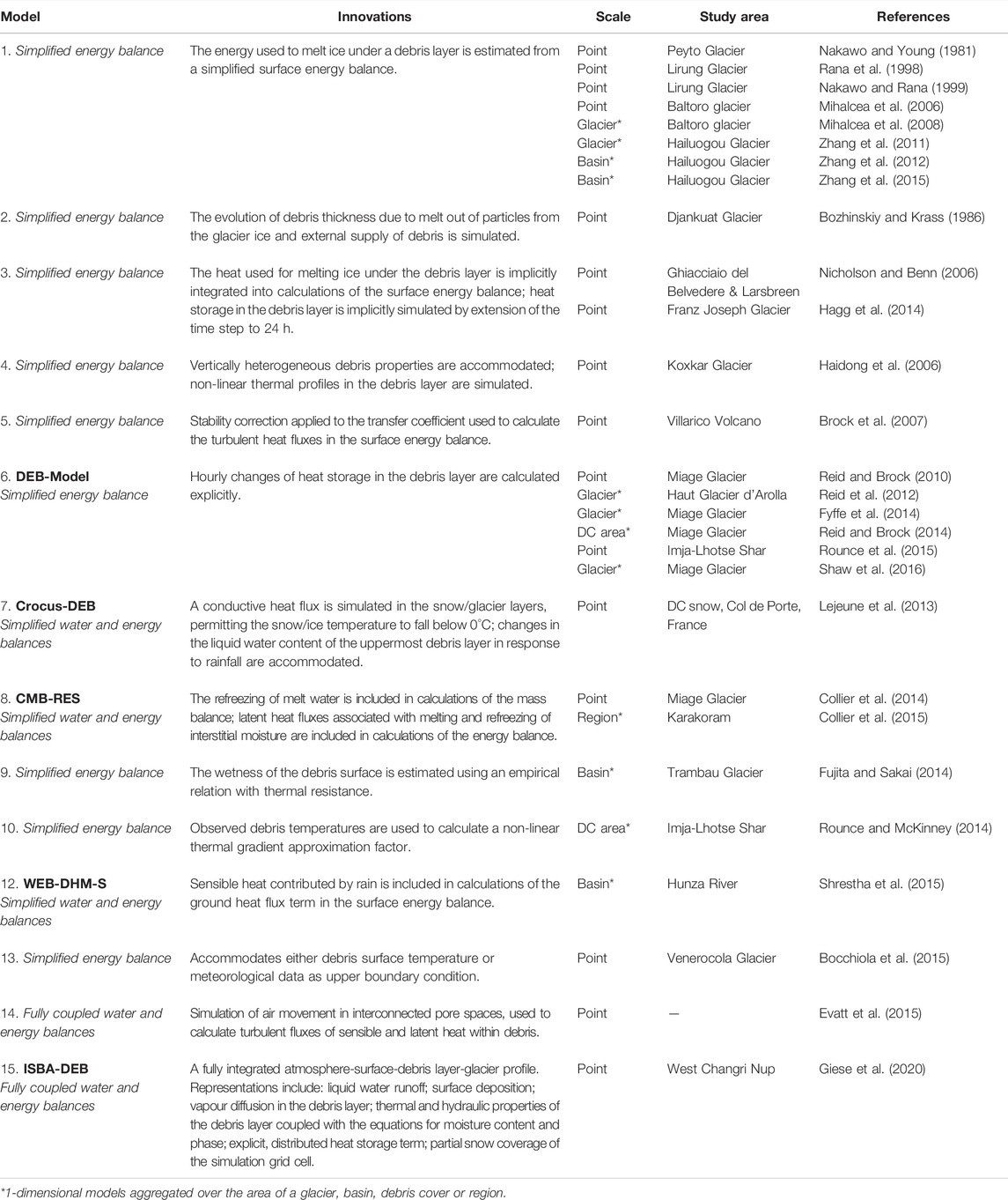
TABLE 1. Physically based models that have been applied to predict ablation of glacier ice under a debris layer. At a minimum, the models listed compute vertical heat conduction through the debris layer. Additional processes involved in melting of glacier ice under a debris layer that are represented in each model have been summarised under the heading Innovations. Groups of models having the same physical representations are listed against a number from 1 to 15, in order of increasing physical completeness. In each of the 15 groups, studies in which the models were applied are listed chronologically by the date of publication. Some of the models were named by their authors, in which case their name is given in bold font under the heading Models.
This paper introduces a new physically based model for predicting sub-debris ice melt that aims to provide the most complete set of process representations to date. The model is based on the Simultaneous Heat and Water (SHAW) transport model for predicting the water and energy balances of soils affected by processes of freeze/thaw, snow cover and/or vegetation at a point-scale (Flerchinger, 1987). SHAW has been widely validated at sites around the world (e.g. Flerchinger et al., 1996; Wang et al., 2010; Flerchinger et al., 2012; Li et al., 2012; Sun et al., 2016; Langford et al., 2020) and is maintained by the United States Department of Agriculture (USDA). SHAW is capable of predicting variables including the depth of soil freezing, latent heat fluxes associated with the phase change of water, snow accumulation and evolution, soil and ice temperatures, and the advection of heat by unfrozen water.
A new version of SHAW, SHAW-Glacier, was developed for this study. It incorporates all of the processes represented within the original model. In addition, SHAW-Glacier simulates energy and moisture fluxes within solid glacier ice, as well as lateral water transport above a solid ice surface and in a porous surface layer of ice.
The specific aims of this study were to 1) demonstrate the extended functionality of SHAW-Glacier using on-site input data from the debris-covered glacier North Changri Nup, 2) assess the sensitivity of predicted sub-debris ablation to uncertainty in the physical parameters, 3) quantify uncertainty in the predictions of sub-debris ablation and debris temperatures, and 4) enhance understanding of sub-debris ablation on North Changri Nup using simulations of the physical processes from SHAW-Glacier.
This manuscript begins with a description of the original SHAW model and its development for application to debris-covered glaciers. Details of the study site and observational data are presented in Section 3. Section 4 outlines the approaches used to test the numerical stability of SHAW-Glacier. Procedures applied to evaluate the sensitivity of predicted ablation to physical parameters, calculate prediction uncertainty, and assess simulations of physical processes made using SHAW-Glacier are outlined in Section 5. Section 6 begins with metrics used to determine a numerically stable model configuration. The simulations of sub-debris ablation are then included with results of the sensitivity and uncertainty analyses, and a selection of output variables with corresponding observations are presented. Section 7 considers the functionality of SHAW-Glacier, and draws insight from the simulations and observations of ablation on North Changri Nup. Section 8 summarises implications of the findings in the context of regional glacier ablation modelling, and finally, suggests new research directions indicated by the findings.
This is the first of a two-part series introducing SHAW-Glacier with its application to North Changri Nup. Part 1 is focused on the overall functionality of SHAW-Glacier with respect to the prediction of sub-debris ablation, and the uncertainty in predicted ablation introduced by the uncertainty in the physical parameter values. The second part of this work will apply SHAW-Glacier to North Changri Nup to explore the influence of patchy snow cover on the variability of sub-debris ablation, with an analysis of heat and water balances simulated under scenarios of wind redistribution (manuscript currently in preparation).
2 The Simultaneous Heat and Water Model
The Simultaneous Heat and Water model, SHAW, is an integrated, one-dimensional surface-subsurface model that was designed to simulate periodically snow-covered and/or frozen soil, with or without vegetation, including permafrost. The energy and water balances are fully coupled, and the atmospheric and sub-surface mass and energy fluxes are fully integrated in the surface mass and energy balance calculations. The physics underlying SHAW and the mathematical representation of the physics are detailed by Flerchinger (1987). For a complete outline of the physics without the mathematical detail, readers are directed to the technical document Flerchinger (2017a) and user manual Flerchinger (2017b).
Since the release of the open-source code, SHAW has been used in applied and academic settings, and it has been validated in studies of continental, maritime, arid and alpine climates in North America, the Tibetan Plateau, North-Central and North-East Asia and western Scandinavia, as well as waste management landfill and laboratory studies. A full list of the publications that report the development, validation and application of SHAW is maintained by the USDA (USDA, 2020).
2.1 Key Features of the Original SHAW Model
SHAW uses meteorological data to simulate the energy, water and solute balances in a 1 m2 column of soil. The column is divided into a maximum of 100 layers. Each layer is assigned a thickness and a set of physical parameter values. The physical parameters represent the characteristics of porous sediment, interstitial air, water and ice, vegetation and vegetation residue if they are present, and snow. The parameters assigned to each layer are fixed within a single run of the model. Computations occur at nodes located at the centre of each layer.
The upper boundary of the simulation is defined by continuous time series of meteorological data. Rain and snow amounts are calculated on the basis of total precipitation, air temperature and relative humidity. The lower boundary is a time series of the moisture content and temperature at the bottom-most node in the simulation profile. The lower boundary for temperature can optionally be estimated by the model as a function of the annual average temperature of the profile at that depth, which is input by the user. The lower boundary condition for soil moisture can optionally be defined as a unit gradient (i.e. gravity flow) beyond the boundary. The initial and final conditions are defined by the moisture content and temperature set by the user for every node in the vertical dimension.
Heat flow within the soil is computed using the solution to the energy balance equation with terms for phase transition for freezing water, advective heat transfer by liquid, and latent heat transfer by vapour. The equation is expressed as:
where Cs and Td are the volumetric heat capacity (J kg−1 °C−1) and the temperature (°C) of the soil, ρi is the density of ice (kg m−3), θi is the volumetric ice content (m3 m−3), ks is the soil thermal conductivity (W m−1 °C−1), z is the positive downward depth from the soil surface, ρl is the density of water (kg m−3), cl is the specific heat capacity of water (J kg−1 °C−1), ql is the liquid water flux (m s−1), qv is the water vapour flux (kg m−2 s−1), and ρv is the vapour density (kg m−3) within the soil. The volumetric heat capacity is computed from the sum of the volumetric heat capacities of the soil constituents, i.e., soil minerals, organic matter, water, ice, and air. SHAW uses the De Vries (1963) approach for computing thermal conductivity.
Water transfer within the soil is solved using the mixed form of the Richards equation with terms for soil freezing, matric-potential-based water flow, vapour transport, and lateral flow exiting the soil column:
where K is the unsaturated hydraulic conductivity (m s−1), ψ is the soil matric potential (m), qlat is the lateral water flow exiting the soil column (m3 m−3 s−1), and U is a source/sink term for water flux (m3 m−3 s−1) that may include lateral inflow and/or root water extraction. Lateral flow exiting the soil column is considered only under saturated conditions (i.e., ψ ≥ 0) and is computed from the slope of the ground surface and the lateral saturated conductivity, KL (m s−1). Unsaturated conductivity within SHAW is reduced linearly with ice content and assumed to be zero when available porosity falls below 0.13 m3 m−3. SHAW provides the option of selecting alternative formulations of the water release curve, but the Campbell equation was used in this study:
where θs is saturated water content (m3 m−3), ψe is air entry matric potential (cm), and b is a pore-size distribution parameter.
As presented in Table 2, SHAW predicts state, flux, and storage terms at the end of every time step of, optionally, 1 hour to 24 h, and at every node. The flux equations are solved in the form of finite differences by an iterative Newton-Raphson technique, with a maximum of 11 iterations per time step. In the case that the equations cannot be solved within the error tolerance, the time step is halved, and the computations are reinitiated within sub-time steps. Time steps are halved for a maximum of 128 sub-time steps per hourly time step.
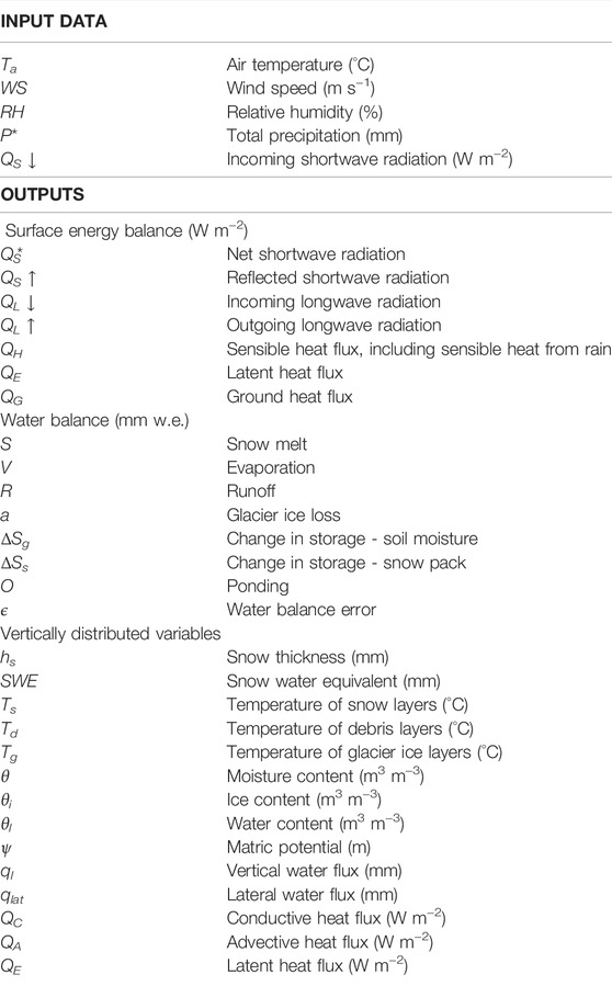
TABLE 2. SHAW-Glacier input data requirements and outputs. Optional outputs relating to vegetation and solute transport are not listed.
2.2 New Representations in SHAW-Glacier
SHAW-Glacier uses the soil layers in SHAW as the basis for the representation of supraglacial debris in SHAW-Glacier. The debris layers are stacked upon one or more layers that have been assigned parameter values representing the characteristics of solid ice (Figure 1). SHAW-Glacier simulates heat transfer at the debris surface, and above and below a debris-ice interface, including an advective heat flux associated with the percolation of liquid water through pore spaces, latent heat exchanges associated with glacier melt and refreezing, and energy transfer between solid glacier ice layers. Lateral flow is calculated during both infiltration and redistribution, so that the lateral flow of water that encounters a barrier, such as a less permeable layer or solid ice, is simulated. Thus, it accounts for downslope lateral flow in a saturated layer perched above the debris-ice interface, and in a porous surface layer of ice.
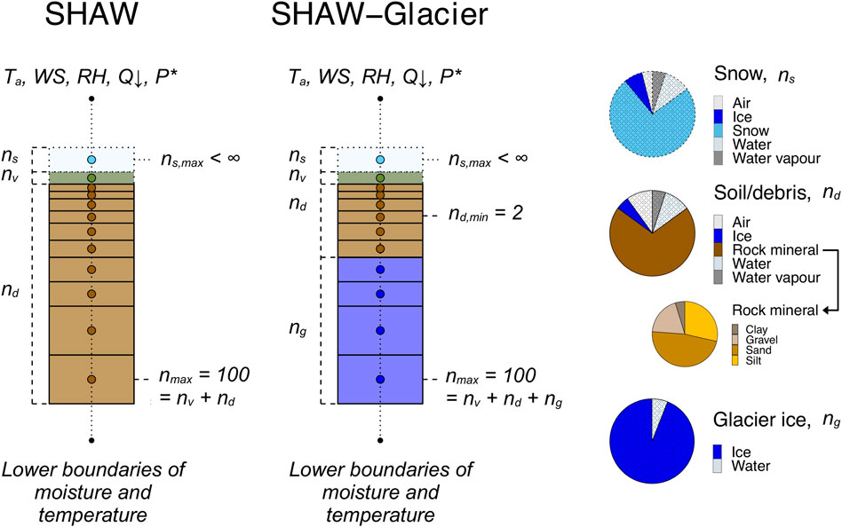
FIGURE 1. A schematic of the simulation domain and process representations in SHAW and SHAW-Glacier. Labels ns, nv, nd and ng are the number of snow, vegetation, debris and glacier ice layers, respectively. Vegetation layers are included under SHAW-Glacier to indicate the model’s functionality, but are not used in this study and therefore, are not included in the detail. Dotted lines in the stacks indicate layers that are time dependent while solid lines represent layers that are constant within a model run. The pie charts show the constituents of the layers; stippling indicates constituents that are time dependent while solid areas are constant. The portions allocated to each constituent in the schematic are for example only.
There are 293 physical parameters in SHAW-Glacier. A user is required to define the value of 28 of those parameters, 30 if snow cover is present upon initialisation. An additional 48 parameters can be user-defined if the simulation is to include plants, plant residue and solute transport. Constants can be changed in the Fortran source code if necessary. There is a complete list of the physical parameters in SHAW in an Appendix to the Technical Document (Flerchinger, 2017a) and of the user-defined parameters in the User’s Manual (Flerchinger, 2017b).
As with SHAW, the maximum number of layers within SHAW-Glacier is 100. The thickness of each debris and glacier ice layer is user-defined, and each layer can be assigned a different thickness. A minimum of two debris or soil layers overlaying the glacier layers is required; the extent of glacier ice below the bottom layer is assumed to be unlimited.
Equations (1)–(3) for heat and water flow through a laterally homogeneous, porous medium are assumed applicable to the glacier layers with slight modifications. The mineral bulk density, ρb (kg m−3), is set to a value from 0.0 (translating to a porosity of 1.0) to 0.1 (i.e. ice with rock mineral content). To maintain the glacier ice layers, a user-defined minimum ice content, θi, min, is specified. As the glacier ice melts, and the ice content of an ice layer falls below θi, min, the ice content is reset to θi, min, and an equivalent amount of water is added to θl to maintain the water balance in the layer. In so doing, it is assumed that the surface of the glacier recedes downward, and the glacier ice beneath the lower boundary is moved upward into the simulation domain.
A maximum water holding capacity, θl, max, is defined for the glacier layers. A low value assigned to θl, max minimises the quantity of liquid water that can be stored in the glacier ice layers despite low values of KS and KL. Within the glacier layers, the value of K(i,t) is independent of changes in θi(i,t). When θl(i,t) ≥ θl, max, K(i,t) is set to KS, and lateral flow from the layer is allowed.
Ablation of the glacier ice,
where ql(NS) and ql(ind) are the liquid water fluxes exiting the bottom and entering the top of the glacier, NS is the total number of debris and ice layers in the simulated profile, ind is an index indicating the first solid ice layer, and Δz(i) is the thickness of ice layer i. Occasionally, ablation of the glacier can be negative as liquid water, ql(ind), enters the top of layer ind and has the opportunity to freeze, adding to the total ice and water content of the ice layers.
Meltwater that is generated at ice layer ind becomes a source of moisture to be drawn into the debris by capillary action. Meltwater that does not soak into the debris is allowed to exit layer ind laterally, as computed by ql, when the water content exceeds θl, max. Refreezing of meltwater can occur in both debris and ice layers, and is included in the water and energy balances.
A weathering crust at the top of the glacier ice can be simulated by setting the water release curve parameters for layer ind to values that are appropriate for a porous material. To the best of the authors’ knowledge, there have been no reports of a weathering crust below a layer of debris, and theoretically, without direct shortwave radiation penetrating below the ice surface, a weathering crust is unlikely to form. However, melt water channels may form under a debris layer, and this feature of SHAW-Glacier may facilitate future studies into the effect of the formation of runnels on sub-debris melt.
In the original SHAW model, the mineral density, ρm (kg m−3), mineral specific heat, cm (J kg−1), and mineral thermal conductivity, km (W m−1 °C−1), for the sand and rock fractions of the soil are constants that are approximately equal to the average for quartz. In SHAW-Glacier, they take user-defined values, which allows the user to evaluate the sensitivity of sub-debris melt to the values of those parameters–e.g. to explore the effect of geology on ablation rates. An option has also been included for the outputs of the energy balance to be calculated by transfer mechanism. The conductive and advective heat fluxes are calculated as the net thermal energy transferred between layers with a reference temperature of 0°C, to allow non-conductive heat sources to be evaluated.
Finally, the maximum number of sub-hourly time steps has been increased from 128 to 512 to assist in numerical convergence. SHAW-Glacier is sensitive to initial and terminal boundary conditions and to the spatial and temporal discretisation scheme, which is discussed below.
2.3 Input Requirements
The input data required to drive SHAW and SHAW-Glacier are the same. Daily or hourly meteorological input data are required to define the upper boundary of a simulation. The input variables are air temperature, relative humidity, wind speed, incoming solar radiation and precipitation. The user can specify rainfall and snowfall amounts separately; alternatively, if only total precipitation data are available, SHAW-Glacier can partition total precipitation into rain and snow amounts based on air temperature and relative humidity.
Albedo of the dry debris surface is an input parameter, αd. SHAW-Glacier calculates the effective surface albedo, α, at every time step to account for wetting of the debris, cloud cover, accumulation of snow, and for the evolution of snow as it ages and melts. Thus, reflected and net shortwave radiation are outputs that are computed.
Initial and terminal thermal and hydraulic boundary conditions must be defined by the user. Observational data can be used to initialise SHAW-Glacier, or in the case that observational data are not available, the simulation can be buffered with a spin-up period to simulate realistic initial profiles of temperature and moisture. The length of the spin-up period required for a given simulation depends on the particular configuration and how well the conditions used to initialise the spin-up reflect reality. The terminal conditions are required to be defined in the input files so that SHAW-Glacier can estimate the temperature and moisture content of the lower boundary if the time series that defines the lower boundary is incomplete.
3 Field Site and Data
3.1 North Changri Nup Glacier
North Changri Nup glacier is a debris-covered alpine valley glacier in the Dudh Koshi basin, Nepal, in the Randolph Glacier Inventory v6.0 (RGI6) region 15, South Asia East (GLIMS ID G086808E28006N and RGI 6.0 ID RGI60–15.03734). North Changri Nup is one of a number of glaciers flowing from the Sagarmatha/Mt Everest massif. The massif has been estimated to be rising at an average of 2 mm yr−1 due to tectonic uplift (Liang et al., 2013) and eroding at up to 4 mm yr−1 (Godard et al., 2014). With plentiful granitic and metamorphic sediment supplied by erosive processes of mass movement from the valley walls (Nakawo et al., 1986), many of the glaciers in the region are debris-covered.
North Changri Nup has an approximate length of 4 km and surface area of 2.7 km2 (Vincent et al., 2016), of which approximately 50%, in the ablation zone, is covered by debris (Herreid and Pellicciotti, 2020). The location of North Changri Nup is illustrated in Figure 2.
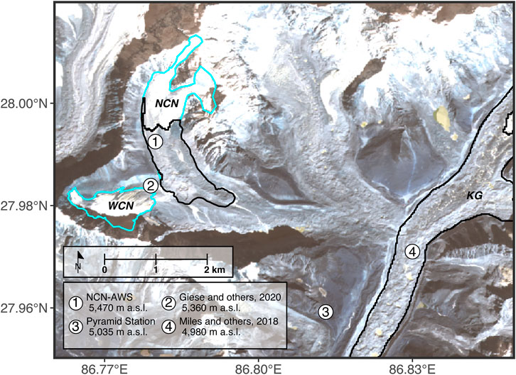
FIGURE 2. Map of the study area. The acronyms WCN, NCN and KG stand for West Changri Nup, North Changri Nup and Khumbu Glacier. The sites where observational data were collected are numbered. The light blue and dark blue polygons are the outlines of the debris-free and debris-covered parts of the glaciers, respectively. The background image is a true colour composite of a Sentinel-2 Product level 1C image that was taken on 27 January 2021.
3.2 Meteorological Input Data
All observational data used in this study were collected within the framework of the global glacier observatory GLACIOCLIM (https://glacioclim.osug.fr/). An automatic weather station, NCN-AWS, was installed in November 2014 and was operational until February 2017 (Figure 3A). The AWS was installed on the debris, at 27.9925° latitude, 86.7799° longitude, 5470 m a.s.l., close to the upper extent of the debris-covered area. Data from the 2016 hydrological year were used, defined as 28 November 2015 to 28 November 2016. A Campbell Scientific CR 1000 datalogger system was installed on the AWS; details of the sensors are listed in Supplementary Table S1. Data from a second AWS that was located on West Changri Nup, WCN-AWS, were used to fill gaps and to correct errors in the data from NCN-AWS. The locations of the two AWS are illustrated in Figure 2, and corrections made to the input data are included in Supplementary Table S1. The data used for the simulations of ablation on North Changri Nup are presented in Figure 4.
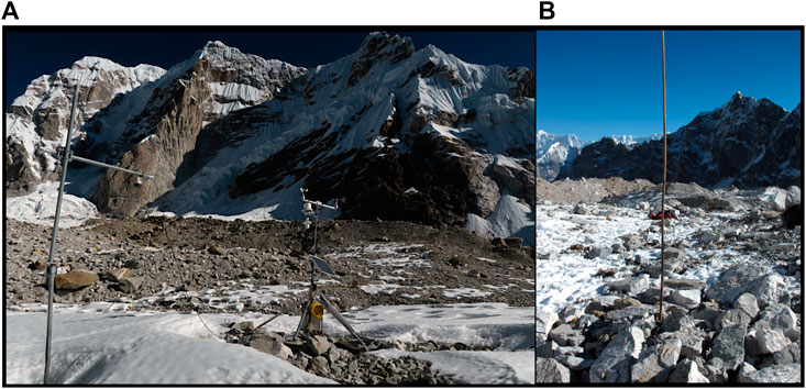
FIGURE 3. (A) NCN-AWS. The photograph shows the relative positions of the sonic ranger and other meteorological instruments, the tilt in the tripod supporting the sonic ranger, and patchy snow cover. (B) One ablation stake in the “stake farm”, showing the natural debris surface. Note the elevated patch of debris around the stake, and patchy snow cover. The photographs were taken on 10 November 2016.
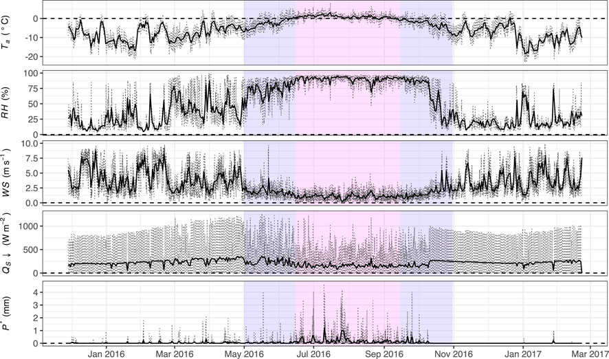
FIGURE 4. Meteorological data used in the modelling study. The dotted lines are hourly values and the solid black lines are daily average values. These data were collected from instruments installed 2 m above the debris surface at NCN-AWS. The background colours indicate the season, as defined by Government of Nepal (2021): white is winter, pink is monsoon, and blue is both pre-monsoon and post-monsoon.
3.3 Glaciological Ablation Data
Point surface mass balance was measured at ten ablation stakes that were installed in an approximately 2500 m2 area around NCN-AWS (Supplementary Figure S1). This “stake farm” was established on 29 November 2014 to observe sub-debris ablation as a function of debris thickness under controlled conditions. The natural debris layer was around 0.08–0.10 m thick, gently undulating, with randomly distributed boulders across the surface. To install each stake, a 2 m diameter patch of debris was excavated and a 4 m long bamboo pole was drilled into the ice at the centre of the patch. Debris of the desired thickness was distributed evenly in the patch around the stake, using naturally occurring material taken from nearby. A photograph of one of the stakes is presented in Figure 3B. The first year of data are described in Vincent et al. (2016). Repeat measurements of the emergence of the stakes were made on 28 November 2015, 1 May 2016 and 10 November 2016. The coordinates, elevation and debris thickness at each stake are listed in Table 3.
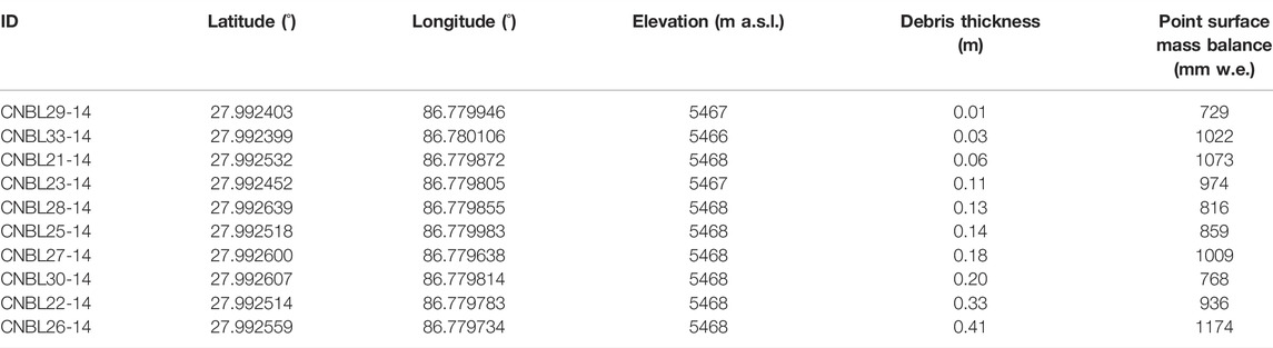
TABLE 3. The locations of ablation stakes installed around NCN-AWS, and point surface mass balance measurements for the period 28 November 2015 to 10 November 2016.
3.4 Observed Debris Temperature
From November 2015, the temperature of the debris layer was recorded at two sites approximately 2 m from NCN-AWS. Two pits were dug into the debris layer, Pit 1 and Pit 2. Thermistors were inserted into the walls of the pits, distributed in profile with as little disturbance to the fabric of the sediments as possible, and the pits were back-filled. The debris in Pit 1 had a thickness, h, of 0.10 m and the thermistors were installed at depths, d, of 0.01, 0.05 and 0.10 m. Pit 2 was 0.08 m thick and thermistors were installed at d = 0.01 m and d = 0.08 m. The thermistor model was TCA PT100, which has an uncertainty of 0.1°C.
3.5 Physical Parameter Values
The physical parameters that allow SHAW-Glacier to simulate solid ice layers were assigned constant values and excluded from the sensitivity and uncertainty analysis. The mineral bulk density, ρb (kg m−3), was set to zero, θi, min to 0.92 m3 m−3 and θl, max to 0.05 m3 m−3. The remaining terms in Eq. (3), ψe and b, were assigned values of -0.01 cm and 1.5, respectively, to minimise accumulation of water in the ice. The hydraulic conductivity of the ice layers was fixed at a value of 0 cm h−1 to preclude vertical transfer of liquid water between the ice layers.
Physical parameters that were well constrained were also excluded from the analyses of sensitivity and uncertainty: measured values of latitude and elevation were used for the site of each ablation stake, while the solar noon hour, estimated from the time zone, was held constant at 12:30. Slope (10%) and aspect (160°) were estimated using the data from the HMA 8 m DEM (Shean, 2017).
A feasible range of values was required for each of the remaining 18 parameters to test the ability of SHAW-Glacier to predict melt given the best available information, and to calculate prediction uncertainty. On-site measurements were not available for any of the parameters, but three measurements from neighbouring glaciers were considered to be applicable to North Changri Nup. Additional observational data were compiled from published studies to define the range that each remaining parameter could reasonably take. The parameters that were varied and the range of values used in the uncertainty analysis are presented in Table 4. The provenance of the values used to define a feasible range for each parameter is detailed in the Supplementary Material, and references for the values obtained from published studies are provided in Supplementary Table S2.
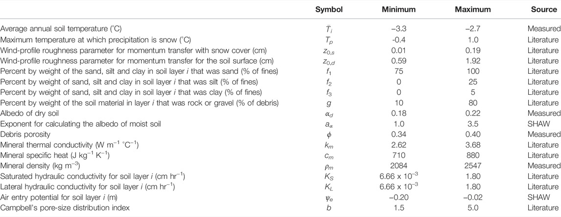
TABLE 4. The parameters in SHAW-Glacier that were included in the sensitivity and uncertainty analysis. The minima and maxima correspond to ±10% of measured values and the lower and upper quartiles of values compiled from published studies. The provenance of the values is expanded upon in the Supplementary Material.
4 Model Stability and Configuration
4.1 Boundary Conditions
Observations of the temperature of the debris in Pit 1 were used to set the initial and terminal thermal conditions. Nodes corresponding to measurement depths were assigned the temperatures recorded in Pit 1 at the dates and times of initialisation and termination. The topmost node of the profile was assigned a temperature that was calculated as the 2-week average of the air temperature recorded at NCN-AWS, and the bottom-most node was assigned a temperature of −3°C, from the data published in Miles et al. (2018). The temperature at the intervening nodes was linearly interpolated between those values.
No data were available with which to define the initial or terminal moisture content of the debris, so assumed values were used. The debris nodes were set to 0.3 m3 m−3, and the glacier ice nodes to 0.92 m3 m−3 to represent solid glacier ice with a density of 0.92 relative to water. Moisture at the lower boundary was estimated by SHAW-Glacier.
The simulation was buffered with periods of dynamic equilibrium spin-up and spin-down (Lamontagne-Hallé et al., 2020) to ensure the predictions would not be biased by the assumed boundary conditions. Tests for numerical stability, detailed in the following section, were used to determine an appropriate spin-up period.
4.2 Determination of a Stable Discretisation Scheme
The stability of SHAW-Glacier was evaluated by performing 100-years runs with different initial thermal conditions and otherwise identical inputs. The 2016 meteorological data from NCN-AWS were looped 100 times to create the input time series. The model configuration was deemed to be stable if the 100-years time series of annual glacier ice mass loss that were predicted using different initial conditions converged to a unique solution, within a reasonable margin of error. Three initial conditions were tested, as follows:
1) Observational: 2-week mean air temperature for the node at the upper boundary, observed debris temperatures at the nodes corresponding to observation depths, and −3°C at the lower boundary, interpolated linearly to intervening nodes.
2) Isothermal: 3°C at every node from the upper to lower boundaries.
3) Observational debris and isothermal ice: 2-week mean air temperature for the node at the upper boundary, observed debris temperatures at the nodes corresponding to observation depths, interpolated to intervening debris nodes, and −3°C at every glacier ice node.
Following standard practice, the time step, Δt, depth interval, L, the maximum number of iterations at each sub-time step, I, and error tolerance, η, were adjusted to identify stable configurations. A total of 144 100-yr simulations were performed, testing every combination of the initial conditions and configuration parameters.
The first 25 years and last 1 year of each run were discarded to account for spin-up and spin-down. The remaining 74 years of predicted annual glacier ice loss of each simulation,
The configuration parameter values that were tested are listed in Supplementary Table S3. The simulated profiles were assigned a total thickness of 50 m, and the depth intervals, L, in the top 1 m of the profile were varied among the tests. The coarsest values of L that were tested, 0.01 and 0.02 m, were distributed evenly. Then, in order to test the effect of L = 0.02 m when the thickness of the debris layer was not divisible by 2, an additional combination was tested in which the topmost layer was assigned a value of L = 0.01 m and the remaining layers in the top 1 m of the profile were assigned L = 0.02 m; this configuration is called ‘L = 0.01 and 0.02 m’ in the analysis below. The remaining 49 m of the profile were divided into layers of increasing thickness with increasing depth, and were the same in every simulation.
5 Sensitivity and Uncertainty Analysis
All data processing and analyses were performed using the R programming language, in RStudio. The packages that were used in addition to base R are listed at the end of the manuscript.
5.1 Monte Carlo Analysis for Physical Parameters
A Monte-Carlo approach was used to assess the sensitivity of predictions of ablation to uncertainty in the physical parameter values, and to estimate parameter uncertainty in
For h = 0.03 m and h = 0.41 m, n was set to 10,000. A smaller number of model runs might have been adequate; for example, Machguth et al. (2008) used n = 5,000 in a Monte Carlo evaluation of the mass balance of Morteratsch Glacier. Machguth et al. (2008) found that the standard deviation of the predictions, and the standard deviation of the standard deviations, stabilised after only 1,000 model runs, and therefore, deemed n = 5, 000 to be robust. In the current study, n was set to 10,000 for the highest and lowest values of h to thoroughly sample the parameter space, and n = 2,000 for 0.03 m
5.2 Recursive Partitioning Based on Predicted Ablation
Recursive partitioning was used to explore modes in the distribution of
The recursive partitioning analysis was performed using the rpart function in the rpart R package (Therneau and Atkinson, 2019). To avoid overfitting the models, the partition trees were pruned with the complexity parameter set to 0.1. Values of annual ablation simulated for the Monte Carlo analysis were grouped according to the results of the recursive partitioning analysis. Prediction uncertainty, Uh,b, was estimated as the difference between the 10th and 90th percentiles of the n values of
5.3 Interpretation of Debris Temperature Observations
Observed temperature at d = 0.01 m in Pits 1 and 2, T0.01,1 and T0.01,2, respectively, was used to infer the presence of snow cover. Positive values of T0.01 and/or distinct diel fluctuations were assumed to indicate an absence of snow, while T0.01 ≤ 0°C coupled with muted diel fluctuations was assumed to indicate the presence of snow.
Snow depth, hs, was calculated using changes in surface height recorded by the sonic ranger at the site of NCN-AWS. It can be seen in Figure 3A that a tilt had developed in the tripod supporting the sonic ranger after the equipment was serviced in May 2016. The tilt would have made the apparent snow depth greater than the true snow depth. The tilt must have developed after 26 July 2016 because there was no net change in hs before that date. Therefore, the values of hs from 01 May to 26 July were taken to be accurate. The magnitude of values of hs from 26 July were disregarded; however, the timing and direction of changes after 26 July were consistent with Ta and P* (Figure 4) and were used to inform the analysis.
An additional 2,000 Monte Carlo simulations were conducted for h = 0.08 m and h = 0.10 m, representing the pits in which thermistors were installed. Predicted snow depth,
A routine was tested in which the parameter for the maximum air temperature at which precipitation can fall as snow, Tp, was varied monthly on the basis of hs. However, agreement between
The sensitivity of
Uncertainties were estimated for
where
Representative examples of the heat and water budgets simulated for h = 0.08 m and h = 0.10 m were used to explore sensitivity in the predicted fluxes. The examples were taken from model runs that produced the median value of
6 Results
6.1 Numerical Stability, Model Configuration and Performance
The numerical stability of SHAW-Glacier was sensitive to all of the configuration parameters that were tested. Numerical stability generally increased with an increase in L, an increase in the maximum number of iterations at each time step, I, and a decrease in the error tolerance, η. The distribution of
Simulations using values of L < 0.01 m consistently suffered fatal non-convergence and were deemed to be unstable. Values of s calculated for
Using the coarser vertical discretisation schemes, L = 0.02 m and L = 0.01 and 0.02 m, in combination with the relaxed error tolerance of η = 1 x 10⁻⁴, the distribution of values of
Diagnostic statistics for the two stable configurations are presented in Supplementary Table S4. Configuration 1, with L = 0.02 m, was used for profiles where h was a multiple of 0.02, and Configuration 2, with L = 0.01 and 0.02 m, was used for profiles where h was not a multiple of 0.02. It is notable that, although both configurations met the criteria for numerical stability, they produced significantly different values of
In the stable 100-yr runs with different initial conditions,
6.2 Sensitivity of Predicted Ablation to Model Parameters
The values of annual ablation predicted in the Monte Carlo simulations followed a multi-modal distribution for every value of h. The recursive partitioning analysis indicated that Tp was the most significant parameter determining branches at both first and second order. The structure of the partition trees was similar among the values of h; the recursive partition tree for h = 0.03 m is presented in Figure 5 (equivalent plots for h = 0.06–0.41 m have been included in Supplementary Figures S3–S11). The first order partition values of Tp that were calculated for each value of h, T1p, ranged from 0.03°C to 0.10°C, with apparently random variation around a mean of 0.06°C. The second order values, T2p, ranged from 0.42°C to 0.62°C, with a mean of 0.53°C (Table 5). At third order, the percent gravel in the debris layer, g, was a significant parameter in addition to Tp for h > 0.03 m. However, the reduction in recursive partitioning error terms was consistently an order of magnitude greater with first order partitioning than it was at higher orders.
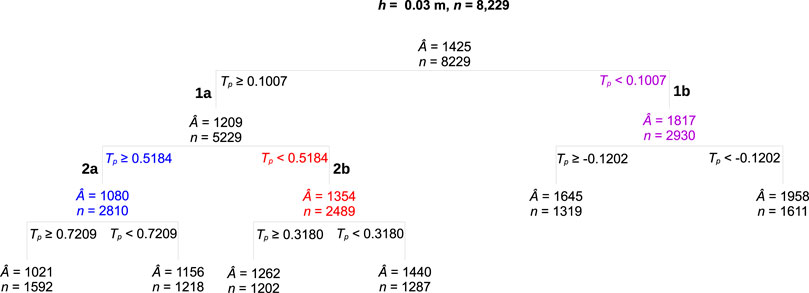
FIGURE 5. Recursive partition tree of annual ablation predicted in the Monte Carlo simulations with debris thickness of 0.03 m. The median values of
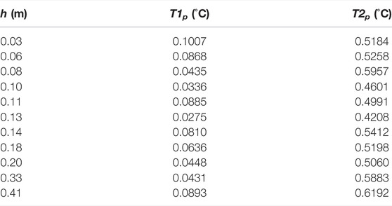
TABLE 5. The first and second order partitioning values fitted for the values of h used in the Monte Carlo simulations of ablation at the sites of the ablation stakes and debris pits.
Grouping the values of
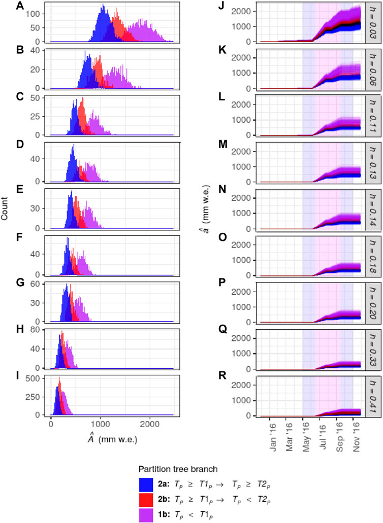
FIGURE 6. Left column: Histograms of predicted annual ablation in 2016,
The characteristic inverse sensitivity of
6.3 Uncertainty in Predictions Associated With Uncertainty in the Parameter Values
Absolute uncertainties were negatively correlated with h (Figure 7). Relative uncertainties increased linearly with debris thickness, from 16% to 40% on branch 2a, 16% to 33% on branch 2b, and 17% to 31% on branch 1b (Supplementary Figure S12). It can be seen in Figure 7 that the difference between the median values on branches 2a and 1b was greater than the range of values on each branch. Therefore, the uncertainty due solely to Tp was greater than the uncertainty due to all of the other parameters, combined.
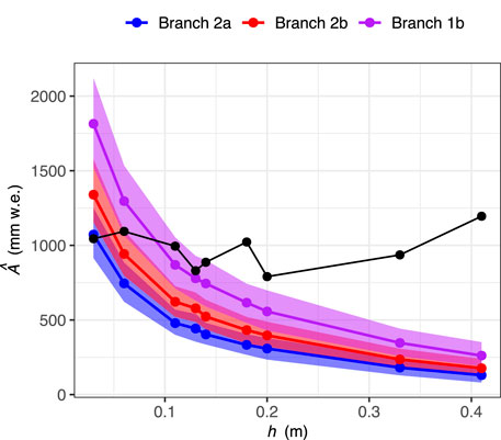
FIGURE 7. Predicted (blue, branch 2a, red, branch 2b, and purple, branch 1b) and observed (black) sub-debris glacier ice ablation for the 2016 hydrological year, plotted against debris thickness. The coloured symbols and lines represent the median values, and the coloured ribbons represent uncertainty bounds based on the 10th and 90th percentiles around the medians.
6.4 Characteristics of the Østrem Curve at North Changri Nup
Annual ablation predicted using SHAW-Glacier followed the characteristic pattern of decreasing magnitude and sensitivity with increasing debris thickness (Figure 7). However, while
6.5 Simulated and Observed Snow Cover
The sensors that recorded T0.01,1, T0.01,2 and hs were located within meters of one another; however, the inferred time series of snow cover were not in agreement. Accumulation occurred simultaneously at the three sites, but complete ablation tended to be asynchronous. Periods with distinct snow cover characteristics, and accumulation events, are labelled P1 - P3 and E1 - E4, respectively, in Figure 8. Table 6 shows that the number of days of snow cover at each site differed during those events. Photographs, such as those presented in Figure 3, showed that snow was distributed in patches in the vicinity of NCN-AWS at the end of the ablation season. The inferred time series were consistent with patchy snow cover.
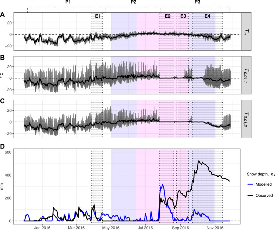
FIGURE 8. (A) Observed air temperature (B) and (C) observed debris temperature at 0.01 m depth in Pits 1 and 2. Grey lines are hourly data and black lines are daily averages. (D) Daily snow depth from the sonic ranger at NCN-AWS (black), and predicted using SHAW-Glacier (blue). Events that are discussed in the text are highlighted with stippling and labelled E1 - E4; labels P1 - P3 refer to periods with distinct snow cover characteristics. The background colours indicate the seasons, as defined by Government of Nepal (2021): white is winter, pink is monsoon, blue is both pre- and post-monsoon.
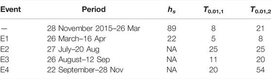
TABLE 6. The number of days of snow cover, during selected events, at the sites of the sonic ranger (hs), Pit 1 (T0.01,1) and Pit 2 (T0.01,2). The events E1 - E4 are highlighted in Figure 8.
Snow depths predicted using SHAW-Glacier are plotted in Figure 8D. In periods P1 and P3, a positive change in
6.6 Sensitivity of Predicted Debris Temperature to Model Parameters
The recursive partition trees for the Monte Carlo simulations with h = 0.08 m and h = 0.10 m had the same structure as the partition trees for the sites of the ablation stakes; the parameter Tp was the most significant at both first and second orders, and g was significant at third order (Supplementary Figure S13, S14). The time series of
The time series of Td,1 and
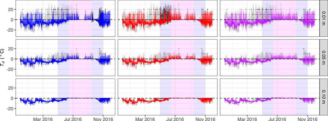
FIGURE 9. Observed debris temperature, Td, at depths d = 0.01, 0.05 and 0.10 m in Pit 1 (stipped black line). Monte Carlo simulations of the same (n = 2,000) have been grouped to second order, with the colour blue used for branch 2a, red for branch 2b and purple for branch 1b.
The simulations on branch 2a of
Grouping the predictions on the basis of
6.7 Ablation Represented in the Simulated Heat and Water Budgets
The simulated heat and water budgets corresponding with the predicted snow cover plotted in Figure 8 have been included in the Supplementary Figures S16, S17. Simulated glacier ice ablation began in June and ended in September for both h = 0.08 m and h = 0.10 m. Through June and July, the magnitude of
Simulated ice ablation occurred only after the snowpack was fully melted. During the pre-monsoon period, snow meltwater, S, was removed by runoff, R, and percolation into the debris, where it contributed to the ground moisture storage term, ΔSg. There was no change in storage of moisture in the debris layer during E2; R closely mirrored S, suggesting the debris had reached field capacity. Once the snowpack had been removed, Sg was reduced by evaporation, and positive values of
7 Discussion
7.1 The Functionality and Performance of SHAW-Glacier
To the authors’ knowledge, SHAW-Glacier is the most complete physical representation of glacier ice ablation under a layer of rock debris. SHAW-Glacier is open-source. A graphical user interface can be used for simple studies, and template input files are available if greater control of the configuration and inputs is required. In this study, the compiled Fortran code was called by scripts written in the R programming language, and run on the terminal through RStudio. On an Apple Macbook Air laptop computer, the length of time to complete a 7 year simulation at hourly resolution varied from 20 s to more than five minutes, depending on the number of outputs being written to file. Manipulating the output comma separated text files was straightforward using functions in base R. Nineteen physical parameters were included in the Monte Carlo analysis, which produced 34,000 water balance and 4,000 temperature profile output files. Using R to open and reformat the 38,000 output files in RStudio, on a system with 2TB RAM, took approximately 14 days.
SHAW-Glacier is sensitive to the configuration of the simulation domain and computation parameters. The frequency of non-convergences was higher when one or more layers was completely frozen. When sediments are near 0°C, small changes in the moisture content and temperature can have an especially large impact on the energy and water balances, because of the interrelated effects of phase changes, latent heat fluxes, permeability and hydraulic conductivity, moisture transport and content. Numerically representing those processes in adjacent saturated and unsaturated layers due to infiltration and percolation of liquid water, freezing and thawing, is a known challenge (Zhang et al., 2010; Lamontagne-Hallé et al., 2020). Non-convergence issues in the current analysis were resolved by increasing the number of computational iterations and decreasing the error tolerance. The configuration required for numerical stability of SHAW-Glacier is likely to vary with the conditions of the study site, such as the meteorological volatility and frequency of sub-surface phase changes, meaning that the flexibility of the discretisation scheme and computing time will vary among studies.
A minimum of two debris layers is required to run SHAW-Glacier. At the current study site, the minimum debris thickness that could be simulated was 0.03 m, because layers assigned values of L < 0.02 m compromised numerical stability. Therefore, it was not possible to evaluate the sensitivity of ablation to debris thinner than 0.03 m at North Changri Nup, nor whether fine debris enhanced ablation rates, i.e. the rising limb of the Østrem Curve. However, it has been estimated that, globally, the median thickness of supraglacial debris cover is 0.15 m (Rounce et al., 2021), meaning that SHAW-Glacier should be functional at the majority of sites world-wide.
SHAW-Glacier successfully modelled the inverse relationship between ablation and debris thickness that defines the falling limb of the Østrem Curve, and the response of
Simulated snow cover could not be validated because the snow cover around NCN-AWS was uneven (discussed below); however, the simulation of debris temperatures showed that SHAW-Glacier accurately represented snow-free and snow-covered conditions (Figure 9). The simulations captured observed diel variation of Td and its attenuation with depth during snow-free conditions. Periods in which snow cover was simulated were identifiable using
The option to include vegetation could be useful in future studies of debris-covered glaciers that have been colonised by plants. For example, communities of trees are established on a lobe of the terminus of Miage Glacier in the Italian Alps (Pelfini et al., 2012). In addition, Satopanth bamak in the Garhwal Himalaya, India, is sparsely vegetated in the lower ablation zone (Singh et al., 2019), first colonisers have been observed on the debris cover of Lirung glacier, Nepal (Kraaijenbrink et al., 2018), and established vegetation has been observed on the terminus of Malaspina Glacier in Alaska (Truffer, 2021). To the best of our knowledge, the impact of plants on sub-debris ablation has not been evaluated, and SHAW-Glacier could be used for this purpose.
7.2 Prediction Uncertainty due to Uncertainty in the Physical Parameter Values
The values of ablation predicted in the Monte Carlo simulations varied by a factor of two to three for each value of h. Uncertainty in the value of Tp contributed more to total uncertainty than all of the remaining parameters, combined, signifying the decisive sensitivity of sub-debris ablation to snow cover.
The non-linear sensitivity of
Ranges of predicted ablation, accounting for uncertainty, did not consistently overlap with observed ablation, indicating that at least one important process was not accurately represented by the parameter values, the structure of the model and/or input data. The uncertainties that were calculated for ̂Td did not account for the observations during periods that the simulation of snow cover was inaccurate. Giese et al. (2020) reported a similar finding: simulations made using the physically based model ISBA-DEB on West Changri Nup were inaccurate when snow cover was not accurately reproduced. In the current study there was evidence that the snow cover had accumulated or ablated unevenly, due to processes that cannot be represented in a 1-dimensional simulation (discussed further below). Neglecting uncertainty relating to uneven deposition or ablation of snow can account for underestimation of the uncertainty in debris temperatures, and may account for the observations of ablation; this hypothesis will be explored in the second part of this study.
Previous research has suggested that sources of uncertainty in predicted sub-debris ablation include properties such as mineral thermal conductivity (e.g. Bocchiola et al., 2015; Evatt et al., 2015), albedo (e.g. Fujita and Sakai, 2014), porosity (e.g. Juen et al., 2013) and surface roughness (e.g. Rounce et al., 2015; Miles et al., 2017; Giese et al., 2020). However, the relative importance of these characteristics is not consistent among studies. In addition to the sensitivity of
7.3 The Sensitivity of Sub-debris Ablation to Snow and Implications of Patchy Snow Cover
The observational data used in this study were unusual, in that ablation was not inversely related to debris thickness (Figure 7). That can be explained by the presence of patchy snow cover during the ablation season. Photographs, as well as the snow depth and debris temperature data, show that there were periods throughout the year when snow was distributed in patches with length scales on the order of centimetres to meters. With some patches of debris covered by snow and others exposed, ablation amounts would be closely related to the duration of the snow, and if patchiness were persistent or frequent, the sensitivity of ablation to debris thickness could be entirely confounded.
Wind redistribution is a feasible mechanism for the development of patchy snow cover at the study site. Patchy snow cover can also form by differential melting and sublimation, but it is deemed unlikely that heat sources varied considerably within the 2500 m2 study area because differences in surface slope, aspect and shading were minor (Supplementary Figure S1). Conversely, micro-topographic features and light winds, which were in evidence, are adequate to cause snow scour and redeposition (Radok, 1977; Dadić et al., 2010). Furthermore, the method used to control the thickness of the debris around each ablation stake produced micro-relief related inversely to debris thickness. That might explain why the sensitivity of observed ablation to debris thickness had the appearance of having been offset systematically. Patches of debris required to be thinner than the naturally occurring debris field were excavated, and thus, depressed relative to the surrounding surface. Patches where the debris was required to be thicker than the natural debris were built up, and thus, elevated relative to the surrounding surface. It is feasible that preferential wind scour occurred where the debris was thick, and preferential deposition where it was thin, producing patches of snow with depths related inversely to debris thickness.
Most glacier melt models operate with grid resolutions of tens to hundreds of meters, and do not simulate sub-grid variability of snow distribution. The results of this study suggest that the variability of snow cover had a stronger influence on ablation than variations in debris thickness. Therefore, development of patchy snow cover during the ablation season could be a source of error in predicted ablation that has not previously been recognized.
Patchy snow cover could be significant over a substantial area. Glacier surface ablation is affected by snow cover during seasonal transitions, around the snowline, and across the ablation zone of summer-accumulation type glaciers. Over 30% of all glaciers outside the polar regions (Braithwaite, 2002) and more than half in High Mountain Asia (HMA) are summer-accumulation type (Ageta and Higuchi, 1984; Sakai et al., 2015). Some proportion of the 10% of glaciers in HMA that are debris-covered (Scherler et al., 2018) lies within the summer-accumulation region. Uneven ablation of fresh snow in the ablation zone could occur routinely on glaciers in that area.
Glaciers in the Sagarmatha/Everest region have all lost mass in the past century. However, projections of the rate of glacier mass loss in the region vary (Sherpa et al., 2017). Summer-accumulation type debris-free glaciers have been found to be more sensitive to air temperature than winter-accumulation type glaciers, because air temperature affects the accumulation and duration of snow during the ablation season (Fujita, 2008; Sakai et al., 2015). In the current study, simulated precipitation phase was more sensitive to Ta during summer, when Ta fluctuated around Tp, than winter, when Ta rarely rose above Tp. It can thus be inferred that
8 Conclusion
This paper has introduced a new physically based model of sub-debris ablation, SHAW-Glacier, which is based on the Simultaneous Heat and Water transport model (SHAW). To the authors’ knowledge, SHAW-Glacier is the most comprehensive physical representation of the processes of sub-debris ablation that has been reported to date, including transfer of rain, meltwater and vapour through the snow-debris-ice column, advection of heat by water, heat fluxes associated with processes of freezing and thawing in the debris, and lateral flow of water through the debris layers and a porous surface layer of ice. The comprehensive representation of physical processes makes SHAW-Glacier useful for evaluating the sensitivity and uncertainty of sub-debris ablation to physical parameters and interactions among them.
In this study, the sensitivity and uncertainty of sub-debris ablation associated with debris thickness and physical parameter values were evaluated by applying SHAW-Glacier to the debris-covered glacier North Changri Nup. Nineteen parameters were varied in a Monte Carlo analysis, and predicted ablation followed the characteristic Østrem Curve. Uncertainties calculated within groups based on the parameter for the maximum air temperature at which precipitation falls as snow increased from 16% to 40% as debris thickness increased from 0.03 m to 0.41 m.
Recursive partitioning revealed that predicted sub-debris ablation was most sensitive to snow cover associated with monsoon precipitation during the ablation season, which has not been previously reported. Indeed, the sensitivity of predicted ablation to snow cover exceeded its sensitivity to debris thickness. Observations of ablation on North Changri Nup, which were unlike any that have been published to date, had no apparent sensitivity to debris thickness. Observed snow cover was patchy during the ablation season, which could have confounded the signal of the sensitivity of ablation to debris thickness by effectively altering the length of the ablation season among the ablation stakes.
Patchy snow cover develops through the redistribution of snow by wind, which is not routinely represented in glacier-melt models at the sub-grid scale. Wind redistribution of snow and patchy snow cover could be sources of uncertainty in regional predictions of ablation, particularly those that encompass high elevation debris-covered glaciers in the monsoon-influenced climate regions of High Mountain Asia.
Further studies to improve understanding of the processes and effects of wind redistribution of snow on sub-debris ablation will be important to constrain the uncertainty introduced to predictions by patchy snow cover. The second part of this study will begin to address that by quantifying the uncertainty introduced to ablation predicted using SHAW-Glacier given scenarios of wind redistribution. In addition, analyses to estimate the geographic extent affected by patchy snow cover during the ablation season, estimate the uncertainty introduced to glacier- and regional-scale predictions of sub-debris ablation by patchy ablation season snow cover, and evaluate the sensitivity of sub-debris ablation to changes in air temperature and precipitation at sites where patchy snow cover occurs, would also be useful to improve projections of debris-covered glacier change.
9 R Packages Used
dplyr (Wickham et al., 2021), here (Müller, 2020), ggforce (Pedersen, 2021), ggplot2 (Wickham, 2016), ggplotify (Yu, 2021), ggpubr (Kassambara, 2020), ggspatial (Dunnington, 2021), ggsn (Santos Baquero, 2019), grDevices (R Core Team, 2021), grid (R Core Team, 2021), gridExtra (Auguie, 2017), magrittr (Bache and Wickham, 2020), raster (Hijmans, 2021), rgdal (Bivand et al., 2021), rpart (Therneau and Atkinson, 2019), RStoolbox (Leutner et al., 2019), rstudioapi (Ushey et al., 2020), sf (Pebesma, 2018).
Data Availability Statement
Publicly available datasets were analyzed in this study. The data can be found here: https://glacioclim.osug.fr/IACS-working-group-on-debris-covered-glaciers-Data-from-West-and-North-Changri.
Author Contributions
SHAW-Glacier was designed and coded by GF. The observational data were collected on field campaigns conducted by PW. The research questions and methodology were designed by AW, RM, RD, GF and AB. AW performed the data analyses. GF drafted Section 2.1. AW drafted all other sections of the manuscript. Editing was performed by RM, RD, PW, GF and AB. All figures were made by AW except the photographs, which were taken by PW.
Funding
Data collection on Changri Nup Glacier has been supported by the French Service d’Observation GLACIOCLIM (part of IR OZCAR), the French National Research Agency (ANR) through ANR-13-SENV-0005-04/05-PRESHINE, and by a grant from Labex OSUG@2020 (Investissements d’avenir–ANR10 LABX56).
Conflict of Interest
The authors declare that the research was conducted in the absence of any commercial or financial relationships that could be construed as a potential conflict of interest.
Publisher’s Note
All claims expressed in this article are solely those of the authors and do not necessarily represent those of their affiliated organizations, or those of the publisher, the editors and the reviewers. Any product that may be evaluated in this article, or claim that may be made by its manufacturer, is not guaranteed or endorsed by the publisher.
Acknowledgments
This study was carried out within the framework of the Ev-K2-CNR Project in collaboration with the Nepal Academy of Science and Technology and Tribhuvan University (JEAI HIMALICE). Thank you to the Associate Editor Martina Barandun, and two anonymous Reviewers, whose feedback and suggestions greatly improved the quality of the manuscript. We appreciate the USDA for maintaining the SHAW model and making it available with supporting documentation. Thanks also to Te Puna Pātiotio Antarctic Research Center, VUW, for supporting AW with visitor access to departmental resources.
Supplementary Material
The Supplementary Material for this article can be found online at: https://www.frontiersin.org/articles/10.3389/feart.2022.796877/full#supplementary-material
References
Ageta, Y., and Higuchi, K. (1984). Estimation of Mass Balance Components of a Summer-Accumulation Type Glacier in the Nepal Himalaya. Geogr. Ann. Ser. A, Phys. Geogr. 66, 249–255. doi:10.1080/04353676.1984.11880113
Auguie, B. (2017). gridExtra: Miscellaneous Functions for ‘Grid’ Graphics. R. package version 2.3. Available at: https://CRAN.R-project.org/package=gridExtra.
Bache, S. M., and Wickham, H. (2020). Magrittr: A Forward-Pipe Operator for R. R. package version 2.0.1. Available at: https://CRAN.R-project.org/package=magrittr.
Bhambri, R., Bolch, T., Chaujar, R. K., and Kulshreshtha, S. C. (2011). Glacier Changes in the Garhwal Himalaya, India, from 1968 to 2006 Based on Remote Sensing. J. Glaciol. 57, 543–556. doi:10.3189/002214311796905604
Biddle, D. (2015). Mapping Debris-Covered Glaciers in the Cordillera Blanca, Peru : an Object-Based Image Analysis Approach. MSc Thesis (Louisville, KY: University of Louisville). doi:10.18297/etd/2220
Bivand, R., Keitt, T., and Rowlingson, B. (2021). Rgdal: Bindings for the ‘Geospatial’ Data Abstraction Library. R. package version 1.5-23. Available at: https://CRAN.R-project.org/package=rgdal.
Bocchiola, D., Senese, A., Mihalcea, C., Mosconi, B., D’Agata, C., Smiraglia, C., et al. (2015). An Ablation Model for Debris-Covered Ice: The Case Study of Venerocolo Glacier (Italian Alps). Geogr. Fis. Din. Quat. 38, 113–128. doi:10.4461/GFDQ.2015.38.11
Bozhinskiy, A. N., Krass, M. S., and Popovnin, V. V. (1986). Role of Debris Cover in the Thermal Physics of Glaciers. J. Glaciol. 32, 255–266. doi:10.3189/s0022143000015598
Braithwaite, R. J. (2002). Glacier Mass Balance: the First 50 Years of International Monitoring. Prog. Phys. Geogr. Earth Environ. 26, 76–95. doi:10.1191/0309133302pp326ra
Brock, B., Rivera, A., Casassa, G., Bown, F., and Acuña, C. (2007). The Surface Energy Balance of an Active Ice-Covered Volcano: Villarrica Volcano, Southern Chile. Ann. Glaciol. 45, 104–114. doi:10.3189/172756407782282372
Bulley, H. N. N., Bishop, M. P., Shroder, J. F., and Haritashya, U. K. (2013). Integration of Classification Tree Analyses and Spatial Metrics to Assess Changes in Supraglacial Lakes in the Karakoram Himalaya. Int. J. Remote Sens. 34, 387–411. doi:10.1080/01431161.2012.705915
Collier, E., Maussion, F., Nicholson, L. I., Mölg, T., Immerzeel, W. W., and Bush, A. B. G. (2015). Impact of Debris Cover on Glacier Ablation and Atmosphere-Glacier Feedbacks in the Karakoram. Cryosphere 9, 1617–1632. doi:10.5194/tc-9-1617-2015
Collier, E., Nicholson, L. I., Brock, B. W., Maussion, F., Essery, R., and Bush, A. B. G. (2014). Representing Moisture Fluxes and Phase Changes in Glacier Debris Cover Using a Reservoir Approach. Cryosphere 8, 1429–1444. doi:10.5194/tc-8-1429-2014
Dadić, R., Mott, R., Lehning, M., and Burlando, P. (2010). Wind Influence on Snow Depth Distribution and Accumulation over Glaciers. J. Geophys. Res. 115, F01012. doi:10.1029/2009JF001261
Dadić, R., Mott, R., Lehning, M., Carenzo, M., Anderson, B., and Mackintosh, A. (2013). Sensitivity of Turbulent Fluxes to Wind Speed over Snow Surfaces in Different Climatic Settings. Adv. Water Resour. 55, 178–189. doi:10.1016/j.advwatres.2012.06.010
De Vries, D. A. (1963). “Thermal Properties of Soil,” in Physics of the Plant Environment. Editor W. R. Van Wijk (Amsterdam: North-Holland Publishing). chap. 7.
Dunnington, D. (2021). Ggspatial: Spatial Data Framework for Ggplot2. R. package version 1.1.5. Available at: https://CRAN.R-project.org/package=ggspatial.
Dussaillant, A., Benito, G., Buytaert, W., Carling, P., Meier, C., and Espinoza, F. (2010). Repeated Glacial-Lake Outburst Floods in Patagonia: an Increasing Hazard? Nat. Hazards 54, 469–481. doi:10.1007/s11069-009-9479-8
Elder, K., Rosenthal, W., and Davis, R. E. (1998). Estimating the Spatial Distribution of Snow Water Equivalence in a Montane Watershed. Hydrol. Process. 12, 1793–1808. doi:10.1002/(sici)1099-1085(199808/09)12:10/11<1793::aid-hyp695>3.0.co;2-k
Evatt, G. W., Abrahams, I. D., Heil, M., Mayer, C., Kingslake, J., Mitchell, S. L., et al. (2015). Glacial Melt under a Porous Debris Layer. J. Glaciol. 61, 825–836. doi:10.3189/2015JoG14J235
Fitzpatrick, N., Radić, V., and Menounos, B. (2017). Surface Energy Balance Closure and Turbulent Flux Parameterization on a Mid-latitude Mountain Glacier, Purcell Mountains, Canada. Front. Earth Sci. 5, 1–20. doi:10.3389/feart.2017.00067
Flerchinger, G. N., Baker, J. M., and Spaans, E. J. A. (1996). A Test of the Radiative Energy Balance of the SHAW Model for Snowcover. Hydrol. Process. 10, 1359–1367. doi:10.1002/(sici)1099-1085(199610)10:10<1359::aid-hyp466>3.0.co;2-n
Flerchinger, G. N., Reba, M. L., and Marks, D. (2012). Measurement of Surface Energy Fluxes from Two Rangeland Sites and Comparison with a Multilayer Canopy Model. J. Hydrometeorol. 13, 1038–1051. doi:10.1175/JHM-D-11-093.1
Flerchinger, G. N. (1987). Simultaneous Heat and Water Model of a Snow-Residue-Soil System. PhD Thesis (Pullman, WA: Washington State University). Available at: https://www.proquest.com/dissertations-theses/simultaneous-heat-water-model-snow-residue-soil/docview/303504656/se-2?accountid=14656.
Flerchinger, G. N. (2017a). The Simultaneous Heat and Water (SHAW) Model: Technical Documentation, in Tech. Rep (Boise, ID: NWRC 2000-09, Northwest Watershed Research Center, USDA Agricultural Research Service). Available at: https://www.ars.usda.gov/ARSUserFiles/20520000/shawdocumentation.pdf.
Flerchinger, G. N. (2017b). The Simultaneous Heat and Water (SHAW) Model: User’s Manual. Version 3.0.X. Tech. Rep. (Boise, ID: NWRC 2017-01.2, Northwest Watershed Research Center, USDA Agricultural Research Service). Available at: https://www.ars.usda.gov/ARSUserFiles/20520500/SHAW/ShawUsers.30x.pdf.
Fujita, K. (2008). Influence of Precipitation Seasonality on Glacier Mass Balance and its Sensitivity to Climate Change. Ann. Glaciol. 48, 88–92. doi:10.3189/172756408784700824
Fujita, K., and Sakai, A. (2014). Modelling Runoff from a Himalayan Debris-Covered Glacier. Hydrol. Earth Syst. Sci. 18, 2679–2694. doi:10.5194/hess-18-2679-2014
Fyffe, C. L., Reid, T. D., Brock, B. W., Kirkbride, M. P., Diolaiuti, G., Smiraglia, C., et al. (2014). A Distributed Energy-Balance Melt Model of an Alpine Debris-Covered Glacier. J. Glaciol. 60, 587–602. doi:10.3189/2014JoG13J148
Giese, A., Boone, A., Wagnon, P., and Hawley, R. (2020). Incorporating Moisture Content in Surface Energy Balance Modeling of a Debris-Covered Glacier. Cryosphere 14, 1555–1577. doi:10.5194/tc-14-1555-2020
Giesen, R. H., and Oerlemans, J. (2013). Climate-model Induced Differences in the 21st Century Global and Regional Glacier Contributions to Sea-Level Rise. Clim. Dyn. 41, 3283–3300. doi:10.1007/s00382-013-1743-7
Godard, V., Bourlès, D. L., Spinabella, F., Burbank, D. W., Bookhagen, B., Fisher, G. B., et al. (2014). Dominance of Tectonics over Climate in Himalayan Denudation. Geology 42, 243–246. doi:10.1130/G35342.1
Government of Nepal (2021). Monsoon Onset and Withdrawal Date Information. Babarmahal, Kathmandu: Ministry of Energy, Water Resource and Irrigation, Department of Hydrology and Meteorology, Climate Division (Climate Analysis Section). Available at: https://www.dhm.gov.np/uploads/climatic/79118284monsoon%20onset%20n%20withdrawal%20English%20final.pdf.
Hagg, W., Brook, M., Mayer, C., and Winkler, S. (2014). A Short-Term Field Experiment on Sub-debris Melt at the Highly Maritime Franz Josef Glacier, Southern Alps, New Zealand. J. Hydrol. 53, 157–165. Available at: https://62397185-821a-4cdf-b4f7-8cc2999495c6.usrfiles.com/ugd/623971_db45e7e64e614163b8b4ed4d055197c5.pdf.
Haidong, H., Yongjing, D., and Shiyin, L. (2006). A Simple Model to Estimate Ice Ablation under a Thick Debris Layer. J. Glaciol. 52, 528–536. doi:10.3189/172756506781828395
Herreid, S., and Pellicciotti, F. (2020). The State of Rock Debris Covering Earth's Glaciers. Nat. Geosci. 13, 621–627. doi:10.1038/s41561-020-0615-0
Hewitt, K. (2014). “Glaciers of the Karakoram Himalaya” in Glacial Environments, Processes, Hazards and Resources (Cham, Switzerland: Springer International Publishing Switzerland). doi:10.1007/978-94-007-6311-1
Hijmans, R. J. (2021). Raster: Geographic Data Analysis and Modeling. R. package version 3.4-10. Available at: https://CRAN.R-project.org/package=raster.
Hock, R., Bliss, A., Marzeion, B., Giesen, R. H., Hirabayashi, Y., Huss, M., et al. (2019). GlacierMIP - A Model Intercomparison of Global-Scale Glacier Mass-Balance Models and Projections. J. Glaciol. 65, 453–467. doi:10.1017/jog.2019.22
Immerzeel, W. W., Lutz, A. F., Andrade, M., Bahl, A., Biemans, H., Bolch, T., et al. (2020). Importance and Vulnerability of the World's Water Towers. Nature 577, 364–369. doi:10.1038/s41586-019-1822-y
Juen, M., Mayer, C., Lambrecht, A., Wirbel, A., and Kueppers, U. (2013). Thermal Properties of a Supraglacial Debris Layer with Respect to Lithology and Grain Size. Geogr. Ann. Ser. A, Phys. Geogr. 95, 197–209. doi:10.1111/geoa.12011
Kassambara, A. (2020). Ggpubr: ‘ggplot2’ Based Publication Ready Plots. R. package version 0.4.0. Available at: https://CRAN.R-project.org/package=ggpubr.
Koppes, M., Rupper, S., Asay, M., and Winter-Billington, A. (2015). Sensitivity of Glacier Runoff Projections to Baseline Climate Data in the Indus River Basin. Front. Earth Sci. 3, 1–14. doi:10.3389/feart.2015.00059
Kraaijenbrink, P. D. A., Shea, J. M., Litt, M., Steiner, J. F., Treichler, D., Koch, I., et al. (2018). Mapping Surface Temperatures on a Debris-Covered Glacier with an Unmanned Aerial Vehicle. Front. Earth Sci. 6, 64. doi:10.3389/feart.2018.00064
Lamontagne‐Hallé, P., McKenzie, J. M., Kurylyk, B. L., Molson, J., and Lyon, L. N. (2020). Guidelines for Cold‐Regions Groundwater Numerical Modeling. WIRES Water 7, 1–26. doi:10.1002/wat2.1467
Langford, J. E., Schincariol, R. A., Nagare, R. M., Quinton, W. L., and Mohammed, A. A. (2020). Transient and Transition Factors in Modeling Permafrost Thaw and Groundwater Flow. Groundwater 58, 258–268. doi:10.1111/gwat.12903
Lejeune, Y., Bertrand, J.-M., Wagnon, P., and Morin, S. (2013). A Physically Based Model of the Year-Round Surface Energy and Mass Balance of Debris-Covered Glaciers. J. Glaciol. 59, 327–344. doi:10.3189/2013JoG12J149
Leutner, B., Horning, N., and Schwalb-Willmann, J. (2019). RStoolbox: Tools for Remote Sensing Data Analysis. R. package version 0.2.6. Available at: https://CRAN.R-project.org/package=RStoolbox.
Li, Z., Ma, L., Flerchinger, G. N., Ahuja, L. R., Wang, H., and Li, Z. (2012). Simulation of Overwinter Soil Water and Soil Temperature with SHAW and RZ-SHAW. Soil Sci. Soc. Am. J. 76, 1548–1563. doi:10.2136/sssaj2011.0434
Liang, S., Gan, W., Shen, C., Xiao, G., Liu, J., Chen, W., et al. (2013). Three-Dimensional Velocity Field of Present-Day Crustal Motion of the Tibetan Plateau Derived from GPS Measurements. J. Geophys. Res. Solid Earth 118, 5722–5732. doi:10.1002/2013JB010503
Lutz, A. F., Immerzeel, W. W., Shrestha, A. B., and Bierkens, M. F. P. (2014). Consistent Increase in High Asia's Runoff Due to Increasing Glacier Melt and Precipitation. Nat. Clim. Change 4, 587–592. doi:10.1038/NCLIMATE2237
Machguth, H., Purves, R. S., Oerlemans, J., Hoelzle, M., and Paul, F. (2008). Exploring Uncertainty in Glacier Mass Balance Modelling with Monte Carlo Simulation. Cryosphere 2, 191–204. doi:10.5194/tc-2-191-2008
Marzeion, B., Hock, R., Anderson, B., Bliss, A., Champollion, N., Fujita, K., et al. (2020). Partitioning the Uncertainty of Ensemble Projections of Global Glacier Mass Change. Earth's Future 8, 1–25. doi:10.1029/2019EF001470
McGrath, D., Sass, L., O'Neel, S., McNeil, C., Candela, S. G., Baker, E. H., et al. (2018). Interannual Snow Accumulation Variability on Glaciers Derived from Repeat, Spatially Extensive Ground-Penetrating Radar Surveys. Cryosphere 12, 3617–3633. doi:10.5194/tc-12-3617-2018
McMahon, A., and Moore, R. D. (2017). Influence of Turbidity and Aeration on the Albedo of Mountain Streams. Hydrol. Process. 31, 4477–4491. doi:10.1002/hyp.11370
Mernild, S. H., Lipscomb, W. H., Bahr, D. B., Radić, V., and Zemp, M. (2013). Global Glacier Changes: A Revised Assessment of Committed Mass Losses and Sampling Uncertainties. Cryosphere 7, 1565–1577. doi:10.5194/tc-7-1565-2013
Mihalcea, C., Mayer, C., Diolaiuti, G., D’Agata, C., Smiraglia, C., Lambrecht, A., et al. (2008). Spatial Distribution of Debris Thickness and Melting from Remote-Sensing and Meteorological Data, at Debris-Covered Baltoro Glacier, Karakoram, Pakistan. Ann. Glaciol. 48, 49–57. doi:10.3189/172756408784700680
Mihalcea, C., Mayer, C., Diolaiuti, G., Lambrecht, A., Smiraglia, C., and Tartari, G. (2006). Ice Ablation and Meteorological Conditions on the Debris-Covered Area of Baltoro Glacier, Karakoram, Pakistan. Ann. Glaciol. 43, 292–300. doi:10.3189/172756406781812104
Miles, E. S., Steiner, J. F., and Brun, F. (2017). Highly Variable Aerodynamic Roughness Length (z0) for a Hummocky Debris-Covered Glacier. J. Geophys. Res. Atmos. 122, 8447–8466. doi:10.1002/2017JD026510
Miles, K. E., Hubbard, B., Quincey, D. J., Miles, E. S., Sherpa, T. C., Rowan, A. V., et al. (2018). Polythermal Structure of a Himalayan Debris-Covered Glacier Revealed by Borehole Thermometry. Sci. Rep. 8, 16825–16829. doi:10.1038/s41598-018-34327-5
Molden, D. J., Shrestha, A. B., Immerzeel, W. W., Maharjan, A., Rasul, G., Wester, P., et al. (2022). “The Great Glacier and Snow-dependent Rivers of Asia and Climate Change: Heading for Troubled Waters,” in Water Security under Climate Change. Editors A. K. Biswas, and C. Tortajada (Singapore: Springer Singapore), 223–250. doi:10.1007/978-981-16-5493-0_12
Müller, K. (2020). Here: A Simpler Way to Find Your Files. R. package version 1.0.1. Available at: https://CRAN.R-project.org/package=here.
Nakawo, M., Iwata, S., Watanabe, O., and Yoshida, M. (1986). Processes Which Distribute Supraglacial Debris on the Khumbu Glacier, Nepal Himalaya. Ann. Glaciol. 8, 129–131. doi:10.3189/s0260305500001294
Nakawo, M., and Rana, B. (1999). Estimate of Ablation Rate of Glacier Ice under a Supraglacial Debris Layer. Geogr. Ann. A 81, 695–701. doi:10.1111/j.0435-3676.1999.00097.x
Nakawo, M., and Young, G. J. (1981). Field Experiments to Determine the Effect of a Debris Layer on Ablation of Glacier Ice. Ann. Glaciol. 2, 85–91. doi:10.3189/172756481794352432
Nicholson, L., and Benn, D. I. (2006). Calculating Ice Melt beneath a Debris Layer Using Meteorological Data. J. Glaciol. 52, 463–470. doi:10.3189/172756506781828584
Panday, P. K., Bulley, H., Haritashya, U., and Ghimire, B. (2011). “Supraglacial Lake Classification in the Everest Region of Nepal Himalaya,” in Geospatial Tech. Manag. Environ. Resour. Editors J. K. Thakur, S. K. Singh, A. L. Ramanathan, M. B. K. Prasad, and W. Gossel (New Delhi: Springer India), 86–99. chap. 6. doi:10.1007/978-94-007-1858-6_6
Pebesma, E. (2018). Simple Features for R: Standardized Support for Spatial Vector Data. R J. 10, 439–446. doi:10.32614/RJ-2018-009
Pedersen, T. L. (2021). Ggforce: Accelerating ‘ggplot2’. R. package version 0.3.3. Available at: https://CRAN.R-project.org/package=ggforce.
Pelfini, M., Diolaiuti, G., Leonelli, G., Bozzoni, M., Bressan, N., Brioschi, D., et al. (2012). The Influence of Glacier Surface Processes on the Short-Term Evolution of Supraglacial Tree Vegetation: The Case Study of the Miage Glacier, Italian Alps. Holocene 22, 847–856. doi:10.1177/0959683611434222
Pritchard, H. D. (2019). Asia’s Shrinking Glaciers Protect Large Populations From Drought Stress. Nature 569, 649–654. doi:10.1038/s41586-019-1240-1
Quincey, D. J., Lucas, R. M., Richardson, S. D., Glasser, N. F., Hambrey, M. J., and Reynolds, J. M. (2005). Optical Remote Sensing Techniques in High-Mountain Environments: Application to Glacial Hazards. Prog. Phys. Geogr. Earth Environ. 29, 475–505. doi:10.1191/0309133305pp456ra
R Core Team (2021). R: A Language and Environment for Statistical Computing. Vienna, Austria: R Foundation for Statistical Computing. Available at: https://www.R-project.org/.
Ragettli, S., Immerzeel, W. W., and Pellicciotti, F. (2016). Contrasting Climate Change Impact on River Flows from High-Altitude Catchments in the Himalayan and Andes Mountains. Proc. Natl. Acad. Sci. U.S.A. 113, 9222–9227. doi:10.1073/pnas.1606526113
Ragettli, S., Pellicciotti, F., Immerzeel, W. W., Miles, E. S., Petersen, L., Heynen, M., et al. (2015). Unraveling the Hydrology of a Himalayan Catchment through Integration of High Resolution In Situ Data and Remote Sensing with an Advanced Simulation Model. Adv. Water Resour. 78, 94–111. doi:10.1016/j.advwatres.2015.01.013
Rana, B., Nakawo, M., Ageta, Y., and Seko, K. (1998). “Glacier Ablation under Debris Cover: Field Observations on Lirung Glacier, Nepal Himalayas,” in International Conference on Ecohydrology of High Mountain Areas. Editors S. Chalise, A. Herrmann, and N. Khanal (Kathmandu: AGRIS), 393–403. Available at: https://lib.icimod.org/record/23011.
Reid, T. D., and Brock, B. W. (2010). An Energy-Balance Model for Debris-Covered Glaciers Including Heat Conduction through the Debris Layer. J. Glaciol. 56, 903–916. doi:10.3189/002214310794457218
Reid, T. D., and Brock, B. W. (2014). Assessing Ice-Cliff Backwasting and its Contribution to Total Ablation of Debris-Covered Miage Glacier, Mont Blanc Massif, Italy. J. Glaciol. 60, 3–13. doi:10.3189/2014JoG13J045
Reid, T. D., Carenzo, M., Pellicciotti, F., and Brock, B. W. (2012). Including Debris Cover Effects in a Distributed Model of Glacier Ablation. J. Geophys. Res. 117 (D18105), 1–15. doi:10.1029/2012JD017795
Rounce, D. R., Hock, R., McNabb, R. W., Millan, R., Sommer, C., Braun, M. H., et al. (2021). Distributed Global Debris Thickness Estimates Reveal Debris Significantly Impacts Glacier Mass Balance. Geophys. Res. Lett. 48 (e2020GL09131), 1–12. doi:10.1029/2020gl091311
Rounce, D. R., and McKinney, D. C. (2014). Debris Thickness of Glaciers in the Everest Area (Nepal Himalaya) Derived from Satellite Imagery Using a Nonlinear Energy Balance Model. Cryosphere 8, 1317–1329. doi:10.5194/tc-8-1317-2014
Rounce, D. R., Quincey, D. J., and McKinney, D. C. (2015). Debris-Covered Glacier Energy Balance Model for Imja-Lhotse Shar Glacier in the Everest Region of Nepal. Cryosphere 9, 2295–2310. doi:10.5194/tc-9-2295-2015
Sakai, A., Nuimura, T., Fujita, K., Takenaka, S., Nagai, H., and Lamsal, D. (2015). Climate Regime of Asian Glaciers Revealed by GAMDAM Glacier Inventory. Cryosphere 9, 865–880. doi:10.5194/tc-9-865-2015
Santos Baquero, O. (2019). Ggsn: North Symbols and Scale Bars for Maps Created with ‘ggplot2’ or ‘ggmap’. R. package version 0.5.0. Available at: https://CRAN.R-project.org/package=ggsn.
Sasaki, O., Noguchi, O., Zhang, Y., Hirabayashi, Y., and Kanae, S. (2016). A Global High-Resolution Map of Debris on Glaciers Derived from Multi-Temporal ASTER Images. Cryosphere Disc. 2016, 1–24. doi:10.5194/tc-2016-222
Scherler, D., Wulf, H., and Gorelick, N. (2018). Global Assessment of Supraglacial Debris-Cover Extents. Geophys. Res. Lett. 45, 11,798–11,805. doi:10.1029/2018GL080158
Shah, S. S., Banerjee, A., Nainwal, H. C., and Shankar, R. (2019). Estimation of the Total Sub-Debris Ablation from Point-Scale Ablation Data on a Debris-Covered Glacier. J. Glaciol. 65, 759–769. doi:10.1017/jog.2019.48
Shaw, T. E., Brock, B. W., Fyffe, C. L., Pellicciotti, F., Rutter, N., and Diotri, F. (2016). Air Temperature Distribution and Energy-Balance Modelling of a Debris-Covered Glacier. J. Glaciol. 62, 185–198. doi:10.1017/jog.2016.31
Shean, D. (2017). “High Mountain Asia 8-meter DEM Mosaics Derived from Optical Imagery, Version 1,” in Dataset, National Snow and Ice Data Center Distributed Active Archive Center, US National Aeronautics and Space Administration. doi:10.5067/KXOVQ9L172S2 Accessed April 20, 2021).
Sherpa, S. F., Wagnon, P., Brun, F., Berthier, E., Vincent, C., Lejeune, Y., et al. (2017). Contrasted Surface Mass Balances of Debris-Free Glaciers Observed between the Southern and the Inner Parts of the Everest Region (2007-15). J. Glaciol. 63, 637–651. doi:10.1017/jog.2017.30
Shrestha, M., Koike, T., Hirabayashi, Y., Xue, Y., Wang, L., Rasul, G., et al. (2015). Integrated Simulation of Snow and Glacier Melt in Water and Energy Balance-Based, Distributed Hydrological Modeling Framework at Hunza River Basin of Pakistan Karakoram Region. J. Geophys. Res. Atmos. 120, 4889–4919. doi:10.1002/2014JD022666
Sun, Z., Wang, Q., Batkhishig, O., and Ouyang, Z. (2016). Relationship between Evapotranspiration and Land Surface Temperature under Energy- and Water-Limited Conditions in Dry and Cold Climates. Adv. Meteorology 2016, 1–9. doi:10.1155/2016/1835487
Therneau, T., and Atkinson, B. (2019). Rpart: Recursive Partitioning and Regression Trees. R. package version 4.1-15. Available at: https://CRAN.R-project.org/package=rpart.
Trubilowicz, J. W., and Moore, R. D. (2017). Quantifying the Role of the Snowpack in Generating Water Available for Run-Off during Rain-On-Snow Events from Snow Pillow Records. Hydrol. Process. 31, 4136–4150. doi:10.1002/hyp.11310
Truffer, M. (2021). Malaspina Glacier: July 2020 Campaign. Available at: https://glacieradventures.blogspot.com/2021/08/malaspina-glacier-july-2020-campaign.html.
USDA (2020). SHAW-Related Publications. Boise, ID: ARS User Files, Agricultural Research Service, United States Department of Agriculture. Available at: https://www.ars.usda.gov/ARSUserFiles/20520500/SHAW/302/SHAWReferences.pdf.
Ushey, K., Allaire, J., Wickham, H., and Ritchie, G. (2020). Rstudioapi: Safely Access the RStudio API. R. package version 0.13. Available at: https://CRAN.R-project.org/package=rstudioapi.
Vincent, C., Wagnon, P., Shea, J. M., Immerzeel, W. W., Kraaijenbrink, P., Shrestha, D., et al. (2016). Reduced Melt on Debris-Covered Glaciers: Investigations from Changri Nup Glacier, Nepal. Cryosphere 10, 1845–1858. doi:10.5194/tc-10-1845-2016
Wang, H., Flerchinger, G. N., Lemke, R., Brandt, K., Goddard, T., and Sprout, C. (2010). Improving SHAW Long-Term Soil Moisture Prediction for Continuous Wheat Rotations, Alberta, Canada. Can. J. Soil. Sci. 90, 37–53. doi:10.4141/CJSS08084
Wickham, H., François, R., Henry, L., and Müller, K. (2021). Dplyr: A Grammar of Data Manipulation. R. package version 1.0.6. Available at: https://CRAN.R-project.org/package=dplyr.
Wickham, H. (2016). Ggplot2: Elegant Graphics for Data Analysis. New York: Springer-Verlag. Available at: https://ggplot2.tidyverse.org.
Williams, H. B., and Koppes, M. N. (2019). A Comparison of Glacial and Paraglacial Denudation Responses to Rapid Glacial Retreat. Ann. Glaciol. 60, 151–164. doi:10.1017/aog.2020.1
Winter-Billington, A., Moore, R. D., and Dadić, R. (2020). Evaluating the Transferability of Empirical Models of Debris-Covered Glacier Melt. J. Glaciol. 66, 978–995. doi:10.1017/jog.2020.57
Yu, G. (2021). Ggplotify: Convert Plot to ‘grob’ or ‘ggplot’ Object. R. package version 0.0.7. Available at: https://CRAN.R-project.org/package=ggplotify.
Zhang, Y., Carey, S. K., Quinton, W. L., Janowicz, J. R., Pomeroy, J. W., and Flerchinger, G. N. (2010). Comparison of Algorithms and Parameterisations for Infiltration into Organic-Covered Permafrost Soils. Hydrol. Earth Syst. Sci. 14, 729–750. doi:10.5194/hess-14-729-2010
Zhang, Y., Fujita, K., Liu, S., Liu, Q., and Nuimura, T. (2011). Distribution of Debris Thickness and its Effect on Ice Melt at Hailuogou Glacier, Southeastern Tibetan Plateau, Using In Situ Surveys and ASTER Imagery. J. Glaciol. 57, 1147–1157. doi:10.3189/002214311798843331
Zhang, Y., Hirabayashi, Y., Liu, Q., and Liu, S. (2015). Glacier Runoff and its Impact in a Highly Glacierized Catchment in the Southeastern Tibetan Plateau: Past and Future Trends. J. Glaciol. 61, 713–730. doi:10.3189/2015JoG14J188
Keywords: glacier, debris, ablation, model, SHAW, physically based, Changri Nup
Citation: Winter-Billington A, Dadić R, Moore RD, Flerchinger G, Wagnon P and Banerjee A (2022) Modelling Debris-Covered Glacier Ablation Using the Simultaneous Heat and Water Transport Model. Part 1: Model Development and Application to North Changri Nup. Front. Earth Sci. 10:796877. doi: 10.3389/feart.2022.796877
Received: 17 October 2021; Accepted: 09 May 2022;
Published: 24 August 2022.
Edited by:
Martina Barandun, Eurac Research, ItalyReviewed by:
Pascal Buri, Swiss Federal Institute for Forest, Snow and Landscape Research (WSL), SwitzerlandThomas Loriaux, Centro de Estudios Científicos, Chile
Copyright © 2022 Winter-Billington, Dadić, Moore, Flerchinger, Wagnon and Banerjee. This is an open-access article distributed under the terms of the Creative Commons Attribution License (CC BY). The use, distribution or reproduction in other forums is permitted, provided the original author(s) and the copyright owner(s) are credited and that the original publication in this journal is cited, in accordance with accepted academic practice. No use, distribution or reproduction is permitted which does not comply with these terms.
*Correspondence: Alex Winter-Billington, winter-billington@alumni.ubc.ca