Kernel Analyses of Volcanic Vent Distribution: How Accurate and Complete are the Objective Bandwidth Selectors?

Kernel Density Estimation is a powerful tool that can be used to extract information about the underlying plumbing system in zones of distributed volcanism. Different approaches concerning the form in which this tool should be applied, however, exist on the literature. One of those approaches sustains that an unbiased selection of a parameter known as the bandwidth is preferable to other alternatives because it reduces biases on the analysis. Nevertheless, there are more than 30 different forms in which a bandwidth can be “objectively” selected, therefore questioning the meaning of “objectivity” on the selection of a method used for its calculation. Furthermore, as shown in this work, the range of allowed “objective” choices of the bandwidth is not much different from a typical range that could be selected subjectively. Consequently, instead of focusing on the question of “what is the best method?” it is shown here that a more informative approach is to focus on the questions of “what are the special values of different methods, and what are their several advantageous applicabilities?”. The benefits of this shift in approach are illustrated with application to three locations of volcanic interest that have a previously well-constrained volcanic structure.

1 Introduction

Statistics and probability are two separate branches of mathematics useful to analyze the relative frequency of events. Statistics involves the description and analysis of the frequency of past events attempting to make sense of observations in the real world, whereas probability deals with predictions concerning the likelihood of future events through the examination of the consequences of mathematical definitions that are issued independently of the real world (Skiena, 2003). When applied to spatial data (i.e., data that can be drawn in a map) statistics includes the generation of summaries describing spatial patterns and can be extended to comparisons between those summaries and expectations raised by theories of how the identified spatial patterns formed (Ripley, 1981). Any attempt to forecasting the spatial location and timing of future events should be considered part of a probabilistic approach. If the objects of interest are volcanic vents, studies involving their spatial distribution can therefore have either a statistical or a probabilistic orientation, depending on the emphasis made on the forecasting component.

There is a vast literature discussing several probability aspects that may produce variable and mutually inconsistent hazard and risk estimates in both seismic and volcanic contexts (e.g., Bernreuter et al., 1988; Marzocchi et al., 2008; Neri et al., 2008; Marzocchi and Bebbington, 2012; Marzocchi and Jordan, 2014; Ake et al., 2018; Bevilacqua et al., 2018; Selva et al., 2019; Marzocchi et al., 2021). Works with a more pronounced statistical approach, however, are not as common (Richardson et al., 2012; Cañón-Tapia, 2014; Cañón-Tapia and Mendoza-Borunda, 2014; Delcamp et al., 2019; Jacobo-Bojórquez and Cañón-Tapia, 2020; Cañón-Tapia, 2021b). It must be remarked that the difference made here between the probabilistic and statistic reports is based on the purpose of the study rather than on the tools used for the presentation of data. This might seem confusing at first because some studies use what would seem to be a statistical tool to assess the hazard of a future eruption (Connor, 1987; Connor and Hill, 1995; Condit and Connor, 1996; Conway et al., 1998; Weller et al., 2006; Jaquet et al., 2008; Connor and Connor, 2009; Kiyosugi et al., 2009; Bebbington and Cronin, 2011; Bebbington, 2015; Connor et al., 2019). Nevertheless, the use of a statistical description within a probabilistic framework is not uncommon, and sometimes is referred by the name of “statistical inference” (DeGroot and Schervish, 2012).

Distinction between the probabilistic and statistic approaches outlined above is important for several reasons, particularly when examining the literature aimed to characterize the spatial distribution of volcanic vents. Motivations for the study of vent distribution in volcanic fields aim to increase our understanding of a wide variety of aspects. To mention but a few those aspects include the relationship existing between polygenetic and monogenetic edifices, geochemical complexities that might arise within a field, the distinction between volcanic events and volcanic edifices, the role played by temporal gaps on volcanic activity or even issues related with the very definition of what is a volcanic field. Readers interested in those particular issues are referred to the works by Valentine and Gregg (2008), Szakács and Cañón-Tapia (2010), Kereszturi and Németh, 2013, Németh and Kereszturi, 2015, Cañón-Tapia (2016), and references therein. Underlying all of those issues at the most general level, the statistical approach aims to present a description of the data (e.g., already existing and identifiable volcanic vents) in such a form that some hypothesis concerning the physical structure leading to the observed distribution can be formulated. In contrast, the probabilistic approach focuses on the identification of the site and time with a larger likelihood for the occurrence of a future event. At a more subtle level, the assumptions made by either a statistically- or a probabilistically-oriented interpretation are also contrastingly different. The statistical interpretation should include assessment of the physical conditions favoring the formation of two or more vents during a single eruption, the orientation of tabular conduits that transport magma to the surface and their relationship with the prevailing stress orientation at the time, the possible shift of location of magma reservoirs, etc. A recent review of these topics, and relevant references are provided by Cañón-Tapia (2021a) and Rivalta et al. (2019). In contrast, a probabilistic or statistical-inference interpretation includes assumptions concerning the type of underlying distribution (Uniform, Clustered, Poisson, etc.), but most importantly it makes assumptions about the equality of likelihood of each outcome (past, present and future) and the continuity of the preferred mathematical distribution both in space and time to validate the interpretations of analysis with respect to a single underlying probabilistic model. Identification of the most basic underlying assumptions in many works, however, are not explicitly discussed. Consequently, it is not surprising that although much effort has been made to characterize vent distribution, it has not been possible to reach a consensus about the methodological approach that guarantees extraction of the larger amount of reliable information from a given set of vents, or even about the type of information that can be obtained under all circumstances.

Failure in understanding the differences between various methodological approaches might result in a negative influence on the scientific and technical acceptability of models which ultimately is detrimental for the advance of scientific knowledge in general. From a practical point of view, the mentioned failure might result in rejection of works submitted to scientific journals on the grounds of alleged errors, ignorance about the method, or indulgence on bespoken methods that produce what the author wants to see. Such statements are difficult to discuss in a formal context because most journals nowadays do not accept the inclusion of references to personal communications or to unpublished works. Nevertheless, those comments play an important role in shaping the evolution of scientific knowledge because acritical acceptance of such statements by some editors leads to rejections of works that are based on alternative methodologies and eliminate the possibility of having a truly open discussion on those subjects. At the end, acceptance of those criticisms followed by rejection of the papers that present alternative methodologies results in the propagation of unilateral points of view that may not have factual support in every circumstance. Although such extreme situations are not the rule across the scientific literature, it is in the best interest of science to reduce the occurrence of such events. This goal can be reached by keeping an open mind capable to work with multiple hypothesis and multiple methodologies to enrich the outcome of scientific enquiry in the most general terms. In addition, it is important to assist the geoscience community to grasp the fundamental aspects of different families of methods developed within theoretical statistics providing landmarks that can be used to assess the possible merits and faults of various works beyond personal opinions.

In this work I focus attention on several aspects of Kernel Density Estimation (KDE) in a volcanic context. Among others, KDE has been used with forecasting purposes in seismology by Frankel (1995) and Hiemer et al. (2014) and in a volcanic context by Connor et al. (2019). Nevertheless, aspects of KDE that have not been treated in detail include: a) the definition of the function used to estimate the probability-density of the data, b) fulfillment in the volcanic context (i.e., the physical world) of the conditions imposed when establishing that function, and c) the possible interpretations of that function in connection with the physical world. Although those issues have been discussed in the natural hazard literature (see references listed above) it would seem that the most fundamental aspects of those issues have not been assimilated by the community at large. Thus, in order to make accessible all of this information to the widest possible audience, the presentation in this work leans towards a more colloquial style. In addition, because the intention of this work is not to finger point any particular work that was produced by adopting alternative approaches than those described below (that judgement is better left to each reader), there are sections of the text that are presented without providing specific references, although the most relevant references are provided in masse. Despite these characteristics, by clarifying here many aspects of KDE that have not been addressed before in the context of the spatial distribution of volcanic vents, it is hoped that the community will have more elements than currently available to make better judgements concerning the conclusions that have been reached whenever this type of methodology has been employed. More importantly, by facilitating comprehension of the several aspects of this method discussed below, it is hoped that not only others might be encouraged to use this powerful tool, but a wider diversity of hypothesis can be generated and tested, ultimately contributing to the better understanding of volcanic systems in general.

2 From KDE Theory to Volcanic Reality

This section presents arguments showing that the most common situations of volcanic interest are likely to involve observations that may not satisfy the assumptions for which KDE was conceived. Aspects examined include the definition of KDE, its interpretation in the context of the physical origin of volcanic vents, and the contrast between the idealized theoretical scenario with the conditions imposed by the real world in volcanic contexts.

2.1 What is Kernel Density Estimation?

KDE encompasses a variety of non-parametric procedures to estimate probability density functions (PDF) associated with a random variable. Despite its name, PDF is a fundamental concept in statistics as defined above (i.e., with no intentions to produce a forecasting of the likelihood of future events). Nevertheless, the normalization of the area beneath that function, inherent to its definition, facilitates its use in statistic-inference realms. In any case, it is important to remark that KDE theory was developed within a statistical context in mind.

Specifically, KDE was developed as a tool for the informal investigation of properties such as skewness and multimodality of the data (Silverman, 1986). As first introduced by Rosenblatt (1956), given a set of N independent observations (x1, x2, x3, … xN), all of which are associated with the same PDF, it is postulated that each of those observations contributes to the definition of a common distribution which can have multiple modes. Thus, in the statistical literature it is common to read that a non-parametric estimator of the PDF can be obtained by evaluating:

$\widehat{f}\left(x\right)=\frac{1}{Nh}{\displaystyle {\sum }_{i=1}^{N}K\left(\frac{x-X_i}{h}\right)}(1)$

at every appropriate value of x. Ironically, the “non-parametric” definition of $\widehat{f}$ includes the parameter h which exerts a strong influence on the calculated PDF. To avoid unnecessary confusion, it is therefore necessary to be aware that the “non-parametric” aspect of $\widehat{f}$ that is alluded in the statistical literature is related to the fact that each PDF calculated with Eq. 1 is obtained without the need to make specific assumptions about parameters such as “mean”, “standard deviation” or “variance”, which are attached to any statistical distribution. The absence of such parameters in Eq. 1 can be verified by noting the fact that on its right hand side we only have the symbols x, K( ), Xi, N and h, none of which represents the mentioned statistical parameters. Indeed, x is one point along a line, one point in a plane, one point in 3-D space, etc. K( ) is a function that needs to satisfy some conditions of continuity, derivability and symmetry, Xi, represents one of the N observations, and h is a different parameter known as the “bandwidth”, “smoothing factor” or “window width”. Furthermore, although it is possible to select K( ) from a wide selection of mathematical functions (common options include Gaussian, Epanechnikov, rectangular, uniform, etc.), all of which satisfy the conditions of continuity, derivability and symmetry, none of those options includes “mean”, “standard deviation” or “variance” as explicit parameters.

Having established the intended meaning of the “non-parametric” adjective when applied to equation 1, it is important to also note that the specific form of K ( ) may lead to some differences in the results. The influence of this selection, however, is not as large as the influence exerted by the parameter h (Cañón-Tapia, 2013). Therefore, selection of K( ) will not be discussed in this paper any more. Instead attention will be focused on the role played by the parameter h.

Selection of a suitable value (or values) of the bandwidth has remained a very controversial subject even within the community specialized in the field of statistics. This topic is treated in more detail in Section 3. Before that, it is important to examine other aspects of KDE that have been the source of some confusion, or that have elicited differences of opinion in volcanic contexts.

2.2 How Suitable are Volcanic Variables to be Analyzed With a Kernel Estimator?

Until now, KDE has been used to characterize vent distributions in zones of distributed volcanism (e.g., Connor, 1987; Connor and Hill, 1995; Lutz and Gutmann, 1995; Condit and Connor, 1996; Conway et al., 1998; Weller et al., 2006; Jaquet et al., 2008; Connor and Connor, 2009; Kiyosugi et al., 2009; Srisutthiyakorn et al., 2010; Bebbington and Cronin, 2011; Richardson et al., 2012; Rose et al., 2013; Cañón-Tapia, 2014; Cañón-Tapia and Mendoza-Borunda, 2014; Bebbington, 2015; Connor et al., 2019; Delcamp et al., 2019; Jacobo-Bojórquez and Cañón-Tapia, 2020; Cañón-Tapia, 2021b; Cañón-Tapia, 2021c). In addition, KDE has also been used to estimate rock/mineral compositions and ages of activity (Bevilacqua et al., 2018; Champion et al., 2018; Marzoli et al., 2018; Stock et al., 2018). Despite this large list of works, there are several aspects embedded in the definition of a kernel that need to be assessed in the specific situation of vent distribution. Five of those aspects are discussed in this section.

2.2.1 Interpretation of the PDF in the Context of the Physical Origin of Vent Distribution

First, it must be noted that the definition of Eq. 1 is valid for cases in which the N observations are all associated with the same PDF that will be estimated. While this is relatively easy to constrain in the context of statistical proofs, where the procedure usually is such that the real PDF is known and the set (or sets) of N observations are drawn from that PDF to test the goodness of the estimator $\widehat{f}$, it is not as easy to be certain that such is the case in the context of volcanic activity. Note that in the previous sentence a distinction has been made between the real PDF (hereafter referred as F) and an estimation of that PDF referred as $\widehat{f}$. Such distinction will be kept in the remainder of this paper.

Returning to the situation presented by volcanic vents, it might be justified to consider that N vents were produced by the same zone of magma storage as indicated by Figure 1A. However, by only looking at the position of vents at the surface it might not be straightforward to say if the observed vent distribution depicts a situation like that shown in Figure 1A (a unique and simple zone of magma storage), Figure 1B (two independent systems overlapping with each other),or Figure 1C (random fluctuations of a unique system that extends deeper beneath the surface). In the first scenario (only one zone of magma storage), the location and shape of the distribution might be controlled by the covering of older vents by younger products, or the lack of enough time to have an adequate statistical sample of the distribution. In the second scenario (two independent, yet overlapping systems) we need to separate N1 observations from system A from the N2 observations of system B, and only then it is justified to estimate the two independent PDFs. In the third scenario (one vertically extensive system with random fluctuations induced by reservoirs at shallower depths) it is justified to consider a mixture of vents emanating from any of the shallow zones of magma storage as part of the same set of N observations and therefore it is justified to calculate a single PDF that should be related to the whole system that includes the different levels of magma storage at different depths, but is equally well justified to attempt to isolate at least the most important intermediate depth reservoirs to gain some insights into the complexity of the volcanic system as a whole. In some circumstances we may be fortunate to have enough information about the composition of all the vents in the region, so that it is possible to be certain which of the three described scenarios is more likely. In most cases of volcanic interest, however, we may not have enough information justifying such a neat separation of vents, and therefore we need to make the analysis considering that there are at least three alternative scenarios that deserve to be evaluated.

FIGURE 1

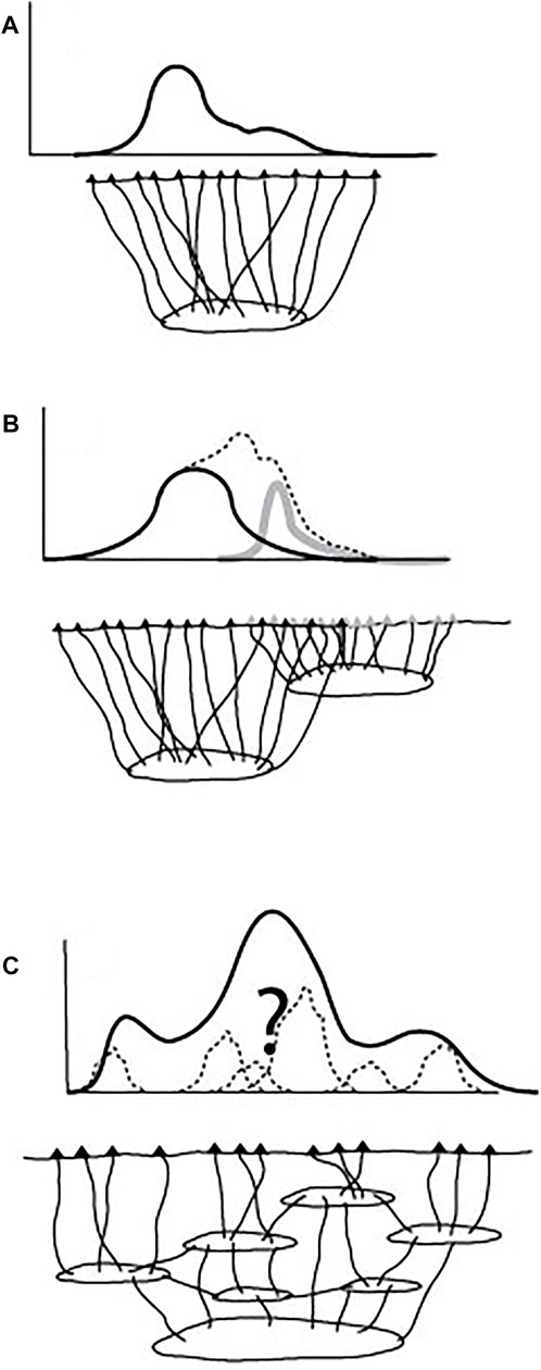
FIGURE 1. Cartoons of three possible scenarios in a region of distributed volcanism and their associated probability density distribution (PDF). In all three scenarios the upper part shows alternative PDFs (solid, dashed or grey lines) and the lower diagram show vents (triangles), zones of magma storage (ellipses) and conduits allowing the vertical transport of magma (lines). The PDFs could be normalized or not, so the vertical axes are left without a label to accommodate both alternatives. (A) All vents are related to one zone of magma storage. Kurtosis and skewness of the distribution (solid line) might be related to inadequate sampling (older vents covered by younger products or immature field not having time to erupt a large enough number of vents). (B) Two overlapping zones of magma storage. Each zone of magma storage produces its own unimodal PDF (solid lines), but they overlap in the central parts of the figure. The shallow zone of magma storage has a PDF with a negative kurtosis and a positive skew (black line), whereas that of the deeper zone tends more to normality, with a slight positive kurtosis (grey line). The dashed line shows a possible combined PDF. (C) a vertically extended zone of magma storage with multiple shallow subsystems. It is uncertain which subsystems have been sufficiently sampled to yield their own PDFs with well-defined characteristics (dashed lines), and which have not. The overall tendency is towards a unimodal PDF (solid line) that reflects the influence of the deeper zone of magma storage, albeit with some noise introduced by the shallower features.

Time is another variable that also needs to be taken into consideration. Its influence, as an independent variable is similar to the influence of composition of the erupted products. Consequently, in the absence of enough time-related information that justifies separation of observations in independent sets, the analysis of the spatial distribution of vents needs to be completed taking in consideration the possibility of the presence of different PDFs within the set of observations. As a result, due to the unknown structure of the buried parts of a volcanic system, assessing the real number of modes that are significant in one PDF obtained from the location of vents is not trivial matter at all. Nevertheless, a thorough analysis must remain open to assess several alternative possibilities.

2.2.2 Density, Intensity and Normalized Values of $\widehat{f}$

A second aspect to be considered from equation 1 is that each $\widehat{f}$ is one estimation of a unique PDF. Due to such a definition, the value of $\widehat{f}$ evaluated at point x is such that it ensures that the integral of the PDF over the whole extension of possible points where it can be evaluated is equal to unity. To some extent, the whole extension to be considered depends on the selection of K( ), but in general it will have a stronger dependence on the value of h selected. Thus, in the strictest sense, the value of $\widehat{f}$ evaluated at a point x does not have a unique relationship with the density of vents defined as the ratio of the number of vents divided by the total area occupied by the volcanic system under scrutiny (which remains constant regardless of the value of h used to define $\widehat{f}$) because each $\widehat{f}$ yields a different fraction at a given point due to the fact that the area to be considered is adjusted as h changes. The relationship with the density of vents is not constant even if visualized as a limiting value because the value at a given point tends to either zero or 1/h when h is smaller than the smaller nearest neighbour distance between any two vents, both of which differ from the constant value defined by the ratio of the number of vents divided by the area occupied by them.

Thus, to avoid the annoying fact that different values of the vent density can be calculated at a given point, depending on the value of h used, $\widehat{f}$ should not be used to quantify vent density in the most intuitive sense of this term. To avoid this type of confusion, the value of $\widehat{f}$ sometimes is referred to as the “intensity”. As explained by Connor and Connor (2009), despite the apparent similarities between intensity and density, both parameters are not entirely equivalent to each other. Nevertheless, the use of intensity is equally problematic because the change of name does not avoid the dependence of h of its calculated value. A much simpler solution seems to refer to the value of $\widehat{f}$ at a given point as the probability-density at that point to remark the association of such value with the statistical origin of the equation used to obtain it. Alternatively, use of normalized values of $\widehat{f}$ (using as a reference the maximum value of $\widehat{f}$ within the zone covered by the observed vents) is a possibility that avoids the need to refer to that number with a specific physical or statistical sense.

2.2.3 Influence of a Small Number of Observations

A third aspect to be considered from Eq. 1 is that even when the definition of $\widehat{f}$ involves a finite number of observations (i.e., N), it is expected that alternative sets, each of N observations, all drawn from the same PDF, should lead to the same, or at least very similar estimator of the common PDF. In the context of pure statistics it is possible to test the goodness of fit of every set of N samples in a straightforward manner because three conditions are satisfied: the real PDF is known, there is an infinite number of possible observations, and there is an equally infinite number of possible combinations of those observations to form the many different sets from which the estimator is calculated. In contrast, in a volcanic context the real PDF is unknown, the number of observations is commonly small, and equally important, there is only one set of observations available to complete an estimation of any PDF. In other words, none of the three conditions assumed to exist to test the goodness of fit is satisfied.

Thus, not only the estimated PDF might be a poor representation of the real PDF despite the method of selection of the bandwidth (due to a small number of related observations, or to a biased sampling, for example), but also the difficulty to make reliable tests with alternative sets of observations is increased because each subset might be even more limited to capture the complexity of the real PDF. This limitation is inherent to the nature of volcanic activity and cannot be overcome by a bootstrap approach because if true representation of the real PDF is not reached by a small number of observations, such a representativity will not be reached by any of the resampled sets. Actually, use of any resampling method might be misleading in those cases because it would provide a false sense of objectivity that is not justified at all, while simultaneously it might overemphasize some bias on the sampling that could have been present in the original set.

2.2.4 Independence of the Observations

A fourth aspect that needs to be taken in consideration is that Eq. 1 was defined for the case of a set of observations that are independent from each other. In most situations of volcanic interest the independence of two vents may not be entirely ensured. Actually, in many cases two or more vents could have been produced by the same eruption and are associated with a common dyke at depth. In those cases, the two vents are not independent observations, and therefore do not satisfy the requirements imposed to the set from which $\widehat{f}$ is calculated. Another aspect relatively common in zones of distributed volcanism is that each eruption changes the availability of magma at depth, as well as it might influence the distribution of stresses between the zone of magma storage and the surface. Although it is difficult to have entire certitude regarding the form in which any eruptive event might change those variables, it can be considered that in general each eruptive event is likely to exert some influence on the location of the next eruption. In any case, the independence of the sampling assumed to characterize the set of observations that serve as the basis for the estimation of the unique PDF will not be fulfilled.

2.2.5 Completeness of the Record

Finally, a fifth aspect worth mentioning is that obliteration of vents due to the most recent eruptions (whether by covering of vents by the new products or by destruction of those vents during the youngest event) as well as the possibility of the occurrence of eruptions that do not leave a clear indication of the vent through which the products were erupted (as for example fissure eruptions that leave feeble traces that are easily eroded or covered by more recent events), also contribute to bring apart the characteristics of the available observations from those assumed to characterize the set of N observations from which $\widehat{f}$ will be estimated.

2.2.6 Implications of the Disparity Between Assumptions and Observations

The arguments presented in this section show that the most common situations of volcanic interest are likely to involve observations that may not satisfy the assumptions for which KDE was conceived. Under those circumstances it is worth to question if it is adequate to complete any analysis of vent distribution using this method. An answer to this question is better postponed until the role played by the smoothing factor has been discussed, and a few illustrative examples have been examined.

3 Estimators of the Bandwidth

After deciding which kernel function K( ) will be used to calculate $\widehat{f}$, it is necessary to decide a value for the parameter h in Eq. 1. The specific choice of K( ) determines the form in which h influences the calculated $\widehat{f}$ as well as the numeric range within which h can be chosen. For example, Cañón-Tapia (2013) showed that Fisher and Gaussian kernels display the exact opposite effect of the calculated $\widehat{f}$ as h is increased; also it was shown that the numerical range of h is entirely different for each kernel. Despite those differences, it was also shown that identical $\widehat{f}$ s can be obtained with both kernels if suitable hs are used in each case. Thus, although the choice of K( ) may not be very large, in order to examine the influence of h it is important to restrict attention to only one type of kernel function.

Thus, to facilitate the discussion, hereafter all calculations will be made with reference to a univariate Gaussian (or normal) kernel. Upon this selection of K( ), Eq. 1 takes the form:

$\widehat{f}\left(x,y\right)=\frac{1}{2\pi N{h}^2}{\displaystyle {\sum }_{i=1}^N\exp \left(-\frac{1}{2}{\left[\frac{d_i}{h}\right]}^2\right)}(2)$

It must be noted that on Equation. 2, $\widehat{f}$ is evaluated at points with coordinates (x, y). Thus, the i-th observation (volcanic vent) has coordinates (Xi, Yi), and is at a distance di from the evaluation point. There are no prescribed units of h, but those units must coincide with the units used to express the separation between vents and evaluation points (i.e., d_i). Coordinates for the vents and evaluation points can be latitude—longitude pairs, in which case distances must be calculated using as a reference a sphere of radius equal to 6,371 km, or another suitable ellipsoid to avoid the effect of curvature of the surface of a planet. If coordinates are given in other systems that already incorporate the effect of the curvature of the surface of the planet (e.g., UTM) the distances can be calculated as they would be in a Cartesian plane, and h can be expressed in either m or km, as deemed convenient.

It is remarked that even when the observations and evaluation points are represented as points in a plane, equation 2 is not strictly bivariate. Indeed, it requires only one variable (the distance between two points) for the calculation of $\widehat{f}$. A truly bivariate form of Eq. 2 can be constructed, but in this case h is not longer a scalar. As explained by Wand and Jones (1993), in a bivariate version of Eq. 2 there can be between one and three independent smoothing parameters that are incorporated as elements of a 2 × 2 matrix. One element is a smoothing factor along the x direction, another element is the smoothing factor along the y direction and the off-diagonal elements on the matrix are equal to each other and allow the resulting $\widehat{f}$ to have axial orientations that are not parallel to the x or y directions. In those cases, if the h-matrix is visualized as representing sample variances, the off-diagonal elements can be visualized as proportional to the covariance between the x and y variances. Other changes to Eq. 2 are required to fully incorporate the effect of increasing the number of dimensions (variables) for which $\widehat{f}$ will be calculated. Nevertheless, the main principle behind Eq. 2 remains unaltered. Consequently, even when attention will be mostly focused on the remainder of this work on examining the effect of h in the univariate kernel represented by Eq. 2, the conclusions remain valid for the fully bivariate kernel, and actually for any kernel applied to higher dimension cases.

In those situations in which the real PDF from which the N observations have been drawn is known (that we should recall has been referred as F), it is reasonable to determine which of the various estimators of $\widehat{f}$ (each obtained with a different h) is the one that better approximates F. The most common approaches to address that issue involve the determination of the difference between the known F and $\widehat{f}$, or the square of that difference. Arguments in favour and against the use of the Integrated Square Error (ISE), the Mean Integrated Square Error (MISE), or the Asymptotic Mean Squared Error (AMISE) as a measure of the difference between F and $\widehat{f}$ have been proposed (Jones, 1991; Jones et al., 1996). Other criteria examined also include the Mean Squared Error (MSE), the Asymptotic MSE (AMSE) and the Sum of the AMSE (SAMSE) (Wand and Jones, 1994; Duong and Hazelton, 2003). In addition to the criteria used to characterize the error, many different approaches have been proposed to minimize those measures of error. The most common methods include variants of Cross-Validation (Least squares, Biased, Smoothed, etc.), variants of Plug-in (Park and Marron, Implemented refined, Bootstrap, etc.), mixing and many other alternatives (Heidenreich et al., 2013). The list is so large that Heidenreich et al. (2013) counted more than 30 bandwidth selection methods, and probably some more have been added since that time. This count relates to bandwidth selectors of univariate kernels. If the methods extend to include bivariate kernels, the number of selectors is even larger. The problem then resides not so much in having one method for the selection of an “optimal”, “objective” bandwidth, but on deciding which method should be chosen (Duong, 2007).

Many comparisons of bandwidth selectors (hereafter referred only as selectors) have been made (Heidenreich et al., 2013; Schindler, 2011; Turlach, 1993 and references therein). Invariably those works have concluded that it has not been possible to find one selector that uniformly performs better than all alternatives when a variety of complex Fs are considered. In practice this indicates that the selector adopted in one situation may or may not have been the best choice, depending on the real F that was under study. In other words, the only possible form to be certain that the selector is the most adequate for the F that needs to be characterized is to know F before making that study. Thus, from a pragmatic point of view it is worth to question, if F is already known, therefore allowing us to calculate very precisely the error of a particular $\widehat{f}$, what is the utility of the calculation of $\widehat{f}$? Furthermore, if F is already known, why should we embark in a series of complex calculations to select only one value of h, that may or may not produce a truly significant $\widehat{f}$, depending on the selector of choice? Similarly, if F is not known with certainty, how can we be certain that a particular $\widehat{f}$ is not significant for the case at hand?

Evidently, it can be argued that any unbiased estimation of h is preferable over a subjective selection of a single h because it should lead to a more robust (stable, reproducible) estimation of $\widehat{f}$, and even when that $\widehat{f}$ may not be an exact determination of the real F, its robustness justifies its selection. Another argument can also be raised in the sense that adoption of the most stable selector increases the possibility of adopting an h that is closer to the real F than the selection of a random h based on purely subjective biases. Although these arguments are not devoid of certain allure, a thorough scientist is likely to ask for more evidence that proves that indeed the real F is better approximated by what is considered to be at that moment the most stable selector. Unfortunately, if the real F is unknown, any argument claiming that a given $\widehat{f}$ is close or far from it results speculative in essence.

To avoid discussions concerning how close a given $\widehat{f}$ might be to an unknown F, it might be convenient to address the issue in a slightly different form. To begin with, it is necessary to realize that trying to decide whether a method for the selection of h based on the AMISE approach is better than one adopting a MISE or SAMSE approach might become a sterile discussion if all the selectors ultimately lead to similar values of h. On the other hand, if different methods lead to very different estimates of h, the discussion of which method should be adopted takes a greater relevance and can be approached from a different perspective. Thus, from a pragmatic point of view, it seems more illustrative to establish to what extent, if any, the selection of the method influences the value of h that is to be inserted in Eq. 2, and most importantly how different are the variously calculated $\widehat{f}$ s.

An indication that the method used to select an “objective” h exerts a large influence on the calculated $\widehat{f}$ is provided by Duong (2007). As shown in Figure 2, the range of possible $\widehat{f}$ s that can be calculated, each with a different h resulting from one specific selector, is particularly large. Although all the $\widehat{f}$ s coincide in identifying a distribution that is elongated in a NW-SE direction, some suggest an elliptical, unimodal distribution, while others indicate bimodality, three main modes, and even a fourth detached mode in the NW corner of the area of study. It is important to remark that the differences amongst the various panels of Figure 2 sometimes represent minute differences in the method employed to select the “optimal” h. For example, all three panels on the left column were obtained with a Plug-in selector that used a SAMSE approach, differing only on the form in which the data and the covariance matrix are used within the selector. Even so, the estimated $\widehat{f}$ s can variously have one, three or four modes.

FIGURE 2

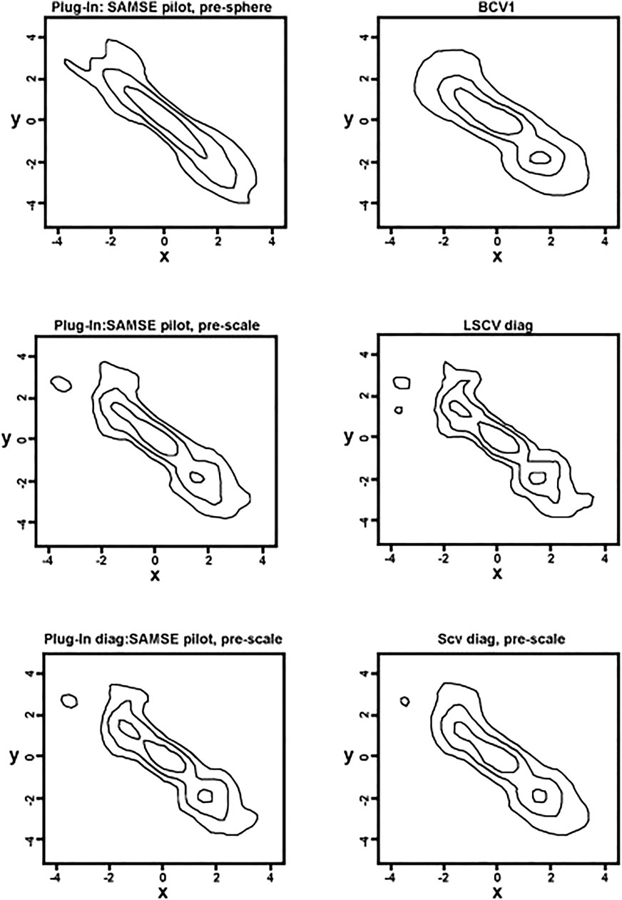
FIGURE 2. Six examples of PDFs calculated with different selectors as indicated on top of each panel. The panels were selected among the examples presented in Figure 2 and Figure 3 of Duong 2007.

The variability of possible results shown in Figure 2, all of which can be claimed to have been calculated in an “unbiased and objective form” indicates that deciding which selector is used turns out to be a subjective choice that includes several assumptions concerning the form in which errors should be handled (MISE, SAMSE, etc.), and even about the specific form of the distribution that underlies the observed group of vents. Thus, whether knowingly or not, the choice of a selector for the bandwidth, and consequently the resulting selection of just one h, are prone to bias. The cumbersome procedure followed and the involvement of a measure of error, however, contribute to disguise such subjective decisions behind an apparently objective choice.

Another important aspect of the results shown in Figure 2 is that there is no form that an outside observer could decide with 100% certainty which $\widehat{f}$ is more accurate (or has less error), because such observer does not know if the real F is unimodal, bimodal, etc. Thus, if a truly unbiased selection of h is to be made where a complex F is expected, as is probably the case in situations of volcanic interest, it would be necessary to test a variety of selectors, all of which claim to be entirely “objective”. The prospective of having to compare the results of a number of bandwidth selectors to decide which is the “more objective”, or the “less biased”, is not that different from the exploratory approach for the selection of h. This approach consists of choosing different values of h to visually inspect the resulting $\widehat{f}$ s (Silverman, 1981). Based on that inspection, a decision can be made about which h is deemed more appropriate, if any. The last remark is important because upon inspection of several estimates of F it might be concluded that more than one h is required to reveal various features of the underlying distribution. Thus, the exploratory method is more akin to the idea of multiple working hypothesis than it is to the uncompromised acceptance of a unique ruling theory (Chamberlin, 1897).

The exploratory approach has been deemed as very dated, also implying that it is undesirable because of its propensity to be affected by a subjective bias (Connor et al., 2019). Nevertheless, as discussed above, due to the diversity of alternative methods for the selection of h, and due to the striking differences that can be obtained from the adoption of even apparently similar methods for that “unbiased” selection, it cannot be asserted that use of a complicated selector is entirely devoid of biases. All things considered, perhaps the only difference is that when the exploratory approach is adopted the subjective choices are on the first plane whereas when an arbitrary selector is favoured the subjective choices are hidden behind the expectations (conscious or subconscious) of the analyst. In consequence, given the fact that subjective decisions are always involved in the selection of either a value of h directly, or through the selection of a method to obtain a supposedly “optimal” h, the merits of the exploration approach should not be dismissed without further examination.

In summary, in this section it has been shown that unless the real distribution from which the vents have been drawn, F, is known with 100% accuracy, it is not possible to decide in an unbiased form which value of h needs to be chosen to minimize the error between the estimated $\widehat{f}$ and the real F. If all things are considered, in a thorough study it is necessary to compare the results of different selectors to ensure that a really significant h is identified. From a pragmatic point of view, it seems much simpler to eliminate the middleman by examining directly several $\widehat{f}$ s obtained with a diversity of values of h. This approach is further explored in the following section.

4 Calibrating the Method in Volcanic Contexts

The theory discussed in the previous section is applied to a few case studies in this section. Thus, in this Section I present the results of the various $\widehat{f}$ s calculated with various selectors available in the environment R available at https://www.r-project.org/. Vent locations from three different zones of volcanic interest were used as input to calculate the corresponding $\widehat{f}$ s. Each of the three zones was selected because there is enough information supporting identification of several key features. Previous geological knowledge about those zones is as close as we can get at this time to knowing the real F. In each of the following subsections several aspects concerning the volcanic systems that should ideally be identified or at least suggested by an analysis of volcanic vent distribution are described before presenting the corresponding $\widehat{f}$ s. Thus, evaluation of the predictive power of the analysis can be made in base of the features that can be identified on each of the calculated $\widehat{f}$ s. It is important to remark that those features have been established from the geologic studies of those zones, and therefore their validity does not depend in any form from the interpretation of the results of vent distributions. Actually, it is precisely because those features have been established from the geology that they can serve as the reference against which the predictions of the kernel method can be compared.

Although there is a large number of selectors that have been advanced in the literature, it is beyond the purpose of this work to make an exhaustive comparison of all of them. Furthermore, as many of those selectors might require access to very specialized programs or to algorithms that might not be easily accessible for the bulk of the geoscience community, the comparison of selectors presented below was restricted to only five. The five selectors included are those available in the generic function “density” of the R environment. These options include nrd0 and nrd which are the rule of thumb proposed by Silverman (1986) and its variation as proposed by Scott (1992), respectively; ucv and bcv, which are unbiased and biased cross-validation methods and sj corresponding to the selector presented by Sheather and Jones (1991). Despite the limited number of selectors presented here, the results serve to illustrate the variability that might characterize the use of different selectors, and therefore suffice to illustrate the main aspect highlighted in the discussion.

All the vent locations used are in Latitude-Longitude pairs, but these are not directly inserted into the functions available in R, which is designed to deal with Cartesian coordinates on a plane. Thus, to avoid issues related to the distortion associated with the shape of the Earth, Latitude-Longitude pairs were converted to UTM before using the density function in R. The resulting hs were then converted to km to produce the diagrams shown in the following sections.

4.1 Mauna Kea, Hawaii

Mauna Kea volcano is one of the five shields that form the Big Island of Hawaii. Its development has followed the same general trends as other Hawaiian large shields, but Mauna Kea is characterized by the presence of a large number of cinder cones along its slopes and close to the summit. Porter (1972) and Wolfe et al. (1997) described the distribution of cinder cones atop Mauna Kea volcano, grouping them in three rift zones, each separated from their neighbors approximately by 120° of arc. In addition to those three rifts, Porter (1972) also mentioned a summit group, and other arcuate or aligned groups randomly located on the slopes of the volcano at various altitudes. According to Porter, some of these linear groups were almost perpendicular to the radial southeast rift, and therefore contributed to diffuse the boundaries of the radial zone, especially in the East. In other words, based on the geology of Mauna Kea volcano it is clear that not all the rift zones are equally developed. The radial East Rift is the best defined of the three near the summit, whereas that on the northeast is the least developed. Still, even the Northeast Rift zone gives a sense of elongation radial to the summit. Most complications are found on the Southeast Rift zone, closer to the base of the larger edifice.

Most of the cones on top of Mauna Kea belong to the Laupahoehoe stratigraphic group, and therefore can be considered to represent examples of coeval activity. Although no claim is made in this work in the sense that all the cones were produced during the same eruption, the relative similarity in age of the cones at least justifies an interpretation in the sense that the ambient regional-tectonic stress should have remained relatively constant. In any case, a distinction based on general composition or age is not granted.

Thus, the things that can be expected to be revealed by an analysis of vent distribution on top of Mauna Kea volcano include: 1) Definition of the three main rifts and the summit groups, 2) Definition or hints about other arcuate groups, and 3) evidence suggesting that all of these vents belong, or at least can be related to one larger system that feeds a central conduit as well as the flank eruptions that formed the three main rifts.

The location of eruptive centers on top and around Mauna Kea were obtained from GoogleEarth, and saved as a MATLAB file, together with a hill-shadow image and georeferenced cell. The image was produced by using a section of the SRTM 1arc_v3 geotif image downloaded from the USGS EarthExplorer server that includes the topography of most of the Big Island. A total of 242 vents were used on the analyses.

The range of h yield by the various selectors goes from 0.9 to 2.5 km (Table 1). As shown in Figure 3, the largest “optimal” h, obtained with the bcv method (Figure 3E), highlights the presence of one large system that has two main subsystems, and probably a third, small one in the southwest corner of the figure. Two of the rift zones can be suspected from the position and shape of the two main subclusters, but the definition of a third rift is not entirely clear. Also, the summit group is not visible at all. In contrast, the smallest “optimal” h, obtained with the ucv method (Figure 3D) allows an immediate identification of the three rift zones and of the summit group. In addition, several groups located mainly on the outskirts of the main edifice are also visible, and distinction of the character of each of the three zones is easy to infer. Nevertheless, this small h does not convey very effectively the sense that all of the various clusters are related to one larger system. In particular, isolated clusters of low probability density on the outskirts of the main edifice fail to be integrated into one larger system. From the intermediate hs, the one obtained with sj (Figure 3F) leads to an $\widehat{f}$ that is close to that of the ucv (Figure 3D), but without as much resolution, especially in what refers to the arcuate, secondary rifts. The other two methods (Figures 3B,C) are closer to the broad resolution offered by the bcv selector (Figure 3E).

TABLE 1

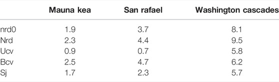
TABLE 1. Optimal bandwidths (in km) selected with five different methods for three areas of distributed volcanism.

FIGURE 3

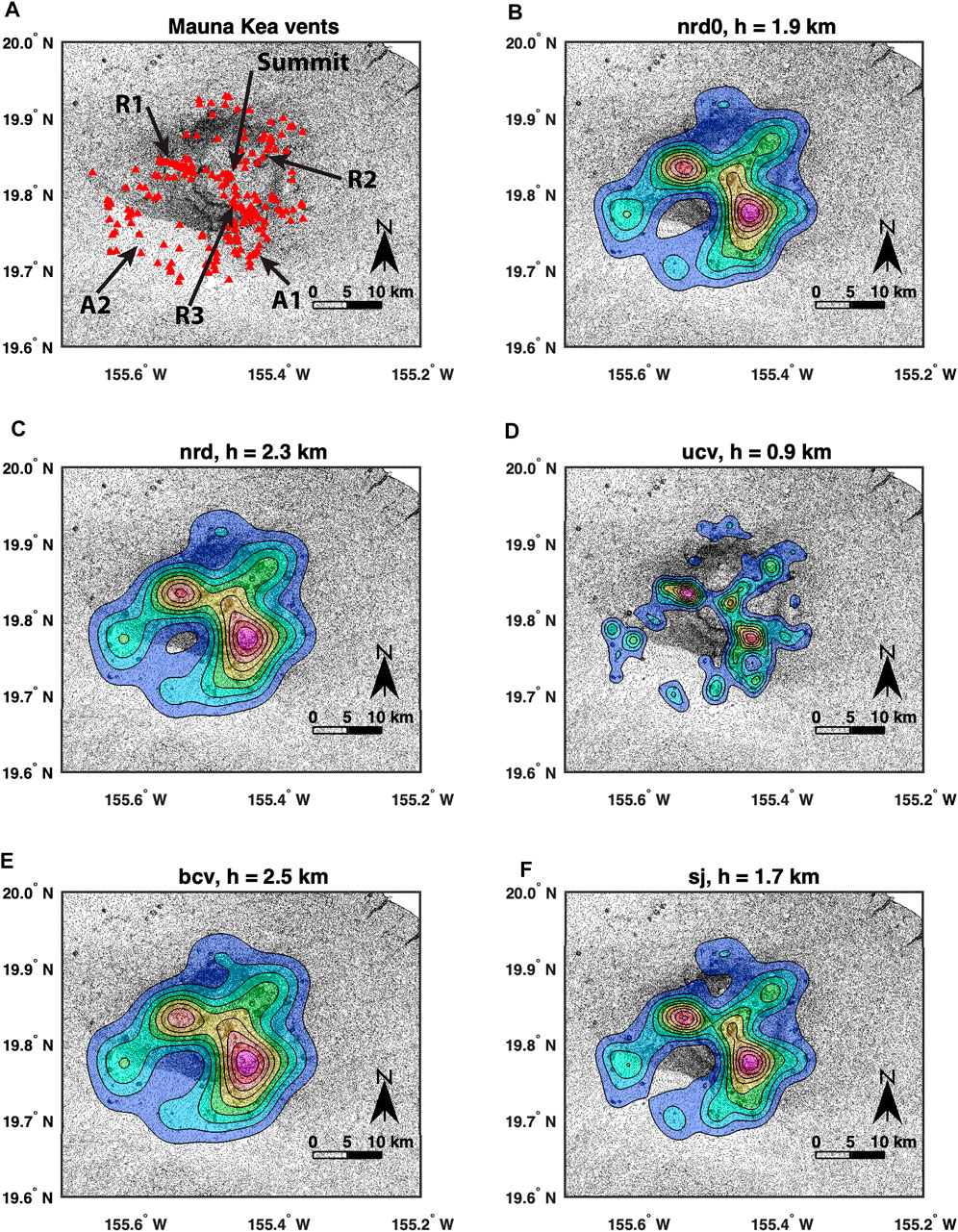
FIGURE 3. Estimated PDFs using the selector and corresponding bandwidth as indicated on top of each panel. The first panel (A) shows the location of the vents used for the calculations. Mauna Kea example.

In summary, the ucv method (Figure 3D) provides the most complete information in this case, but even so, it fails to convey the idea of a unique larger system. All the other options convey that message of a unique system but lack enough resolution to allow clear identification of its main features. It is remarked that none of the calculated hs leads to erroneous interpretations.

4.2 San Rafael Volcanic Field, Colorado

The San Rafael region, Colorado Plateau (western United States) provides a good example of a zone of distributed volcanism where dykes are not associated with a single, central conduit, and where the spatial relationship between dykes and volcanoes can be observed directly at the surface due to the effects of erosion. In this work I used the locations of 62 conduits identified by Kiyosugi et al. (2012). Based on the measurements made in the field by those authors, it is well documented that the dykes have a preferred orientation along a NW-SE direction. Also, based on the described field relations it is clear than many vents have a direct relationship with the larger sills identified in the field. Thus, the things that can be expected to be revealed by an analysis of vent distribution in the San Rafael area include: 1) The most prevalent association that exists between vents and the larger sills, and 2) the regional orientation of stress as indicated by the orientation of dykes and/or sills.

The range of h yield by the various selectors goes from 0.7 to 4.7 km. As shown in Figure 4, the largest “optimal” h, again obtained with the bcv method (Figure 4E), suggests the presence of one roughly elliptical zone of influence with a general NE-SW orientation and two subclusters that loosely coincide in location with the foci of the rough ellipsoid. In contrast the smallest “optimal” h, again obtained with the ucv method (Figure 4D), yields a large number of local maxima that correspond to independent clusters of small dimensions, some of which actually enclose only one or two of the individual volcanoes. Two of the remaining $\widehat{f}$ s are very similar to that associated with the bcv method. The $\widehat{f}$ associated with the sj method ((Figure 4F) allows identification of two main groups, each with characteristic orientation and shape, plus another two smaller sections that tend to have some independence from the largest two. In this case, the three $\widehat{f}$ s, associated with the larger estimates of h tend to yield incomplete and misleading information relative to what is observed in the field. In particular, the NE-SW orientation and connection between the only two maxima in the distribution is an artifact resulting from the neighbourhood of the two main clusters, each with its own field-supported orientation. This is clearly observed on the $\widehat{f}$ associated with the sj method (Figure 4F), where the Northeast group is clearly elongated on the N-S direction, while the Southwest group has an E-W elongation. Also, the position of one of the smaller magnitude maxima at the SW corner contributes to the elongation of the main, oversmoothed feature obtained with larger hs. The $\widehat{f}$ associated with the ucv method (Figure 4D) provides little more information than it would be obtained if only the vent locations were examined. Thus in the San Rafael region the sj method yields an $\widehat{f}$ that contains accurate but incomplete information about the volcanic system. All the other $\widehat{f}$ s are prone to results that are at odds with the exposed part of the field.

FIGURE 4

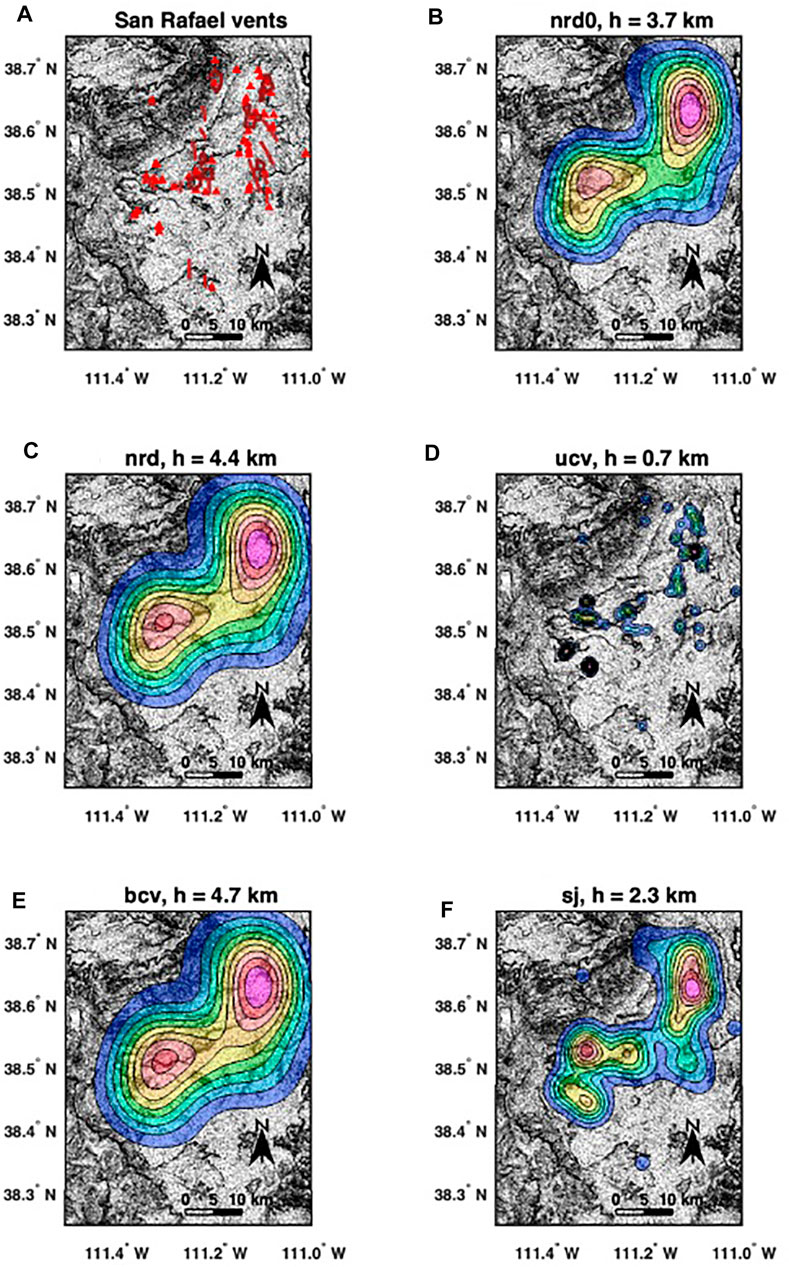
FIGURE 4. Estimated PDFs using the selector and corresponding bandwidth as indicated on top of each panel. The first panel (A) shows the location of the vents used for the calculations (red triangles); the dykes and sills identified by Kiyosugi et al. (2012) are indicated with the red lines. San Rafael example.

4.3 Washington Cascades

The segment of the Cascades located between Mount Rainier and Mount Hood includes a large number of volcanic vents, some of which are large stratovolcanoes and some of which are small, monogenetic cinder cones. A general description of the area is provided by Hildreth (2007) and details of each of the groupings identified can be found on the references therein. From a tectonic point of view volcanism can be divided in three main groups. These include the main axial belt (from Mount Hood to Bumping Lake), a fore-arc section and a back-arc section. The axial belt may be subdivided in three or four sections, each dominated by a larger structure that also comprises several smaller vents. The larger structures in this belt are Mount Hood to the south, Mount Adams in the middle and Goat Rocks to the north. A less prominent structure is Jennies Butte, located between Mt Adams and Goat Rocks, slightly off axis towards the back-arc region. The fore arc section can be also divided in four to seven groups, depending on the emphasis made on the distribution. The main groups in the fore-arc are Mt Rainier to the north, Mt St Helens, Indian Heaven and a zone of diffuse volcanism. The zone of diffuse volcanism itself can be considered to be formed by three distinctive groups (Portland, Wind River and Blue Lake). Finally, the back-arc region is composed by vents of the Simcoe Mountains that may have a north -south division based on the age of the vents. The identification of groups in this area proved to be elusive when out-of-the box clustering methods were employed in isolation. Nevertheless, when the results of several of those methods were combined to define common group associations, the main geological divisions could be identified (Cañón-Tapia, 2020).

The things that can be expected to be revealed by an analysis of vent distribution in this area include: 1) the presence of the most important groups of vents, 2) the North- South orientation and/or distribution of some of those groups, especially in the arc-section, and 3) the different character of the various groups that can be identified. The location of the vents used in this case is the same as that used in a previous report (Cañón-Tapia, 2020).

The range of h yielded by the various selectors goes from 5.7 to 9.5 km. As shown in Figure 5, the largest “optimal” h, obtained with nrd method (Figure 5C), suggests the presence of five clusters, two of which are much more prominent than the other three. The two prominent groups have different orientations, and those two orientations are also reflected on the independent orientations of the less prominent groups. The location of the groups roughly coincides with the location of five of the known groups: three in the center of the map (Santa Helena, a combination of Indian Heaven-Mt Adams, and Simcoe Mountains), and two on the south (Portland area and Mount Hood). All of these groups are still visible, and actually better defined, on the $\widehat{f}$ associated with the smallest estimated h (obtained with the sj method, Figure 5F). In particular, the shared Indian Heaven-Mount Adams group is clearly formed by two semi-independent maxima, both with a predominant N-S orientation. Also, the Portland area is divided in two zones roughly corresponding to the Portland and Wind River groups. In this diagram it is also more evident the presence of an elongated group that extends north and south of Mt Adams, as well as another small group in the position of the Blue-Lake field.

FIGURE 5

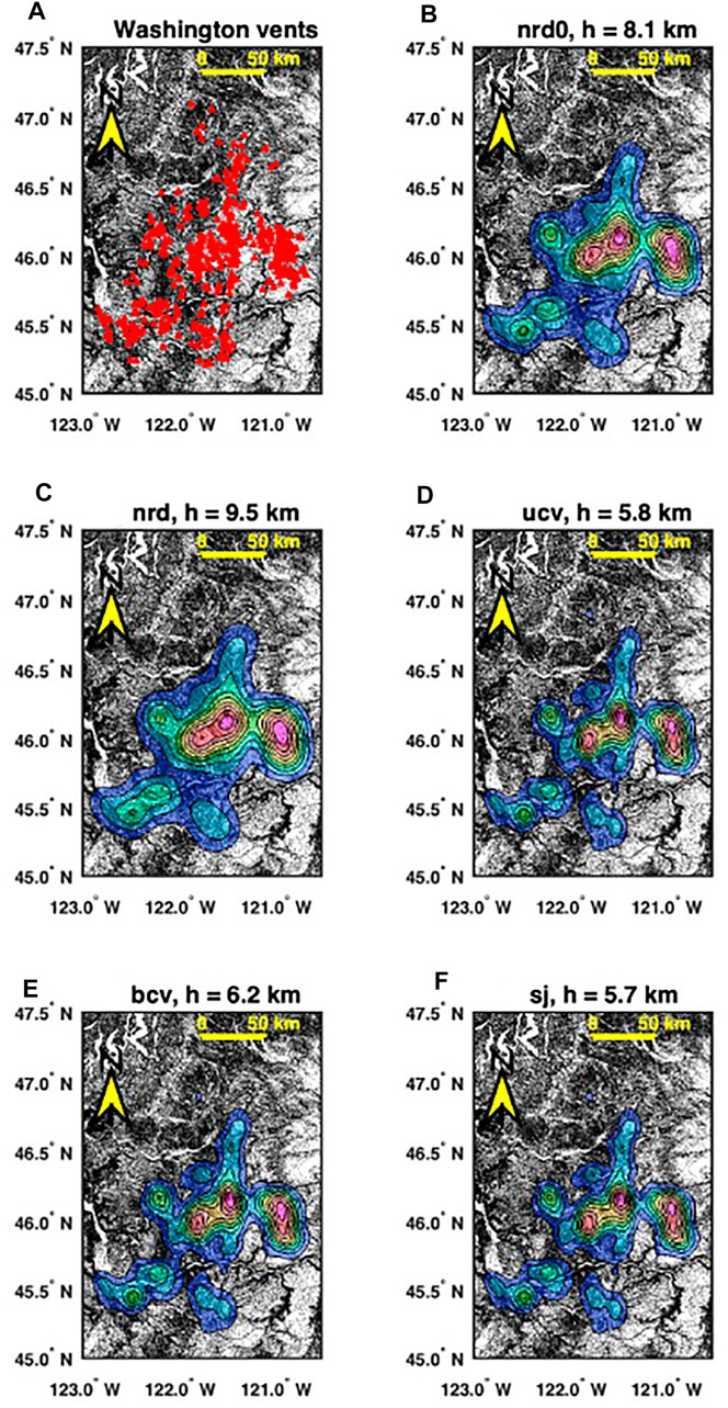
FIGURE 5. Estimated PDFs using the selector and corresponding bandwidth as indicated on top of each panel. The first panel (A) shows the location of the vents used for the calculations (red triangles). Washington Cascades example.

None of the diagrams provides enough information suggesting a possible east-west distinction between fore-arc, arc and back-arc settings. Also, none of the diagrams shows all the main groups with clarity. Furthermore, somewhat misleading information about the expected groups is provided by several diagrams, especially when the fore-arc is fused in the same group as the arc volcanoes.

5 Discussion

5.1 Is There a Better Bandwidth Selector?

As it has been the case when different selectors are compared to each other within the parameters of statistical theory, none of the selectors examined above yield consistently better results than all its competitors. For the case of Mauna Kea the more complete image of the volcanic system was conveyed by the ucv selector, whereas in the San Rafael case the less ambiguous image was provided by the sj selector. In the case of the Washington Cascades none of the selectors did a good job in capturing the complexities of the region. Numerically, the range of bandwidths was ample in all three examples, and none of the selectors systematically yields the smallest or largest value. Perhaps more importantly, while in the Mauna Kea case all the selectors convey an incomplete but correct image of the volcanic system, some of the selectors lead to wrong conclusions in the San Rafael example. Also, ambiguous information is conveyed for the case of the Washington Cascades. Thus, albeit reduced in number, these three examples indicate that there is not a better selector that can be used in each and every case of volcanic interest.

5.2 Alternatives to Bandwidth Selectors

Although it can be argued that the sj method was relatively better because it provided somewhat reliable information in all three of studied locations, it is also clear that the information provided by the corresponding $\widehat{f}$ s was not complete from the geological point of view in any of those cases. This is consistent with the conclusion reached by Bebbington (2013), the sense that some estimators might be more robust at the expense of missing useful information. Certainly, it is the prerogative of every researcher to be as limited as she/he wants to be, and was this the only option available, it would not be an unreasonable one. Nevertheless, as shown next, a thorough investigation that benefits of not missing useful information is also possible.

Table 1 summarizes the values of h that were found by each selector in each of the three scenarios examined. As shown in the Table, the difference between the largest and smallest value of h does not depend in a simple form of neither the number of observations or the size of the area of study. Also, the largest, smallest or middle values of h are not consistently related to a particular selector. Consequently, it is almost impossible to identify a universal rule to decide which selector is the more appropriate for all type of volcanic scenarios, or even if one selector is likely to yield a bandwidth that is smaller, larger or intermediate in relation to other selectors. Based on the descriptions provided in the previous section, however, if instead of focusing attention on only one $\widehat{f}$, all the range of estimated $\widehat{f}$ s is examined, almost all of the relevant features of each of the three regions will be identified. To make this feature clear, Figures 6–8 show a progression of $\widehat{f}$ s obtained with increasing values of h for the Mauna Kea, San Rafael and Washington Cascades cases, respectively.

FIGURE 6

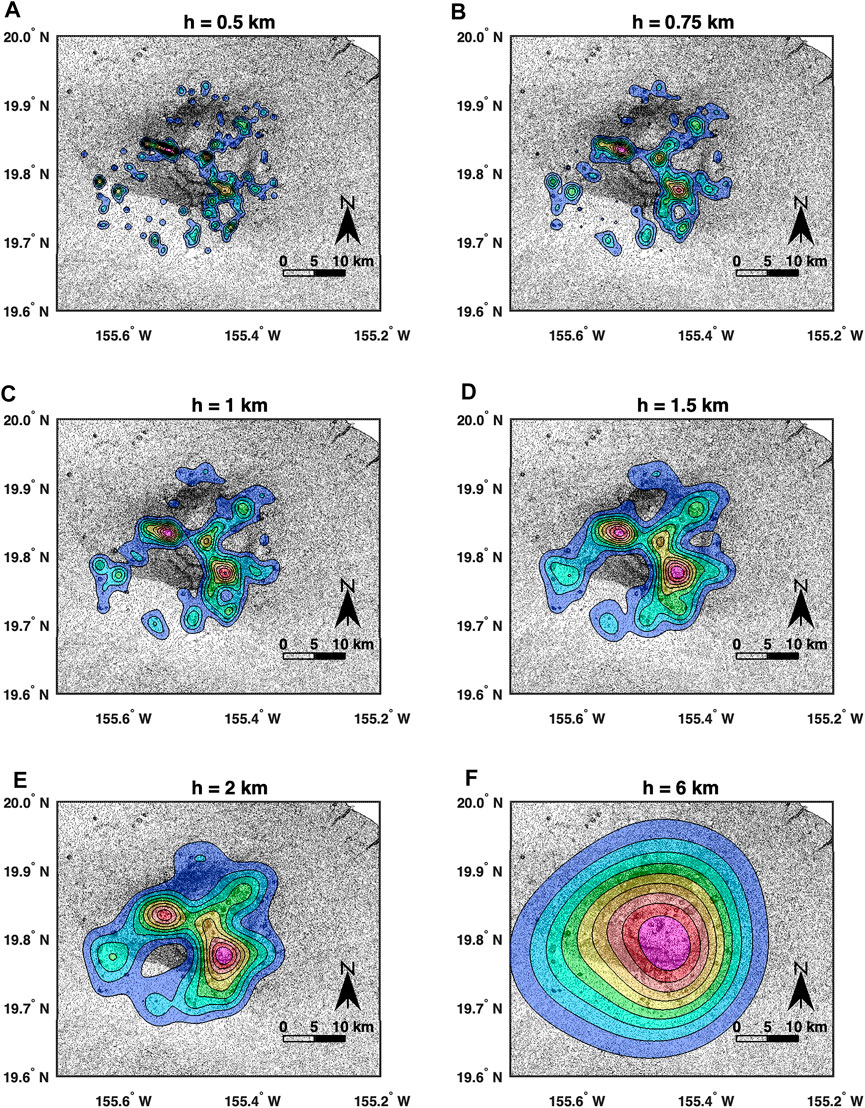
FIGURE 6. Sequence of PDFs used for exploration of the main features of the PDFs associated with the vent distribution of vents atop Mauna Kea volcano.

FIGURE 7

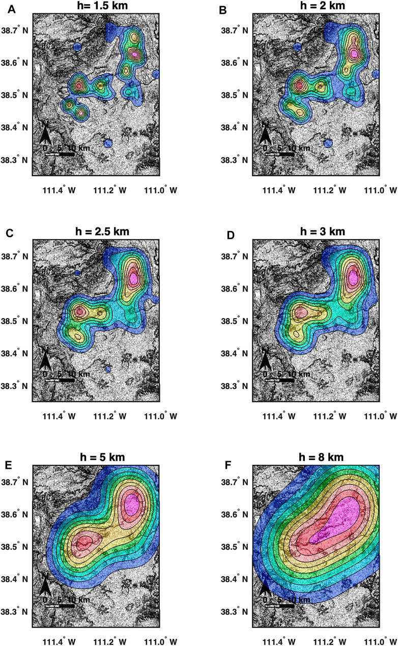
FIGURE 7. Sequence of PDFs used for exploration of the main features of the PDFs associated with the vent distribution of vents on the San Rafael area.

FIGURE 8

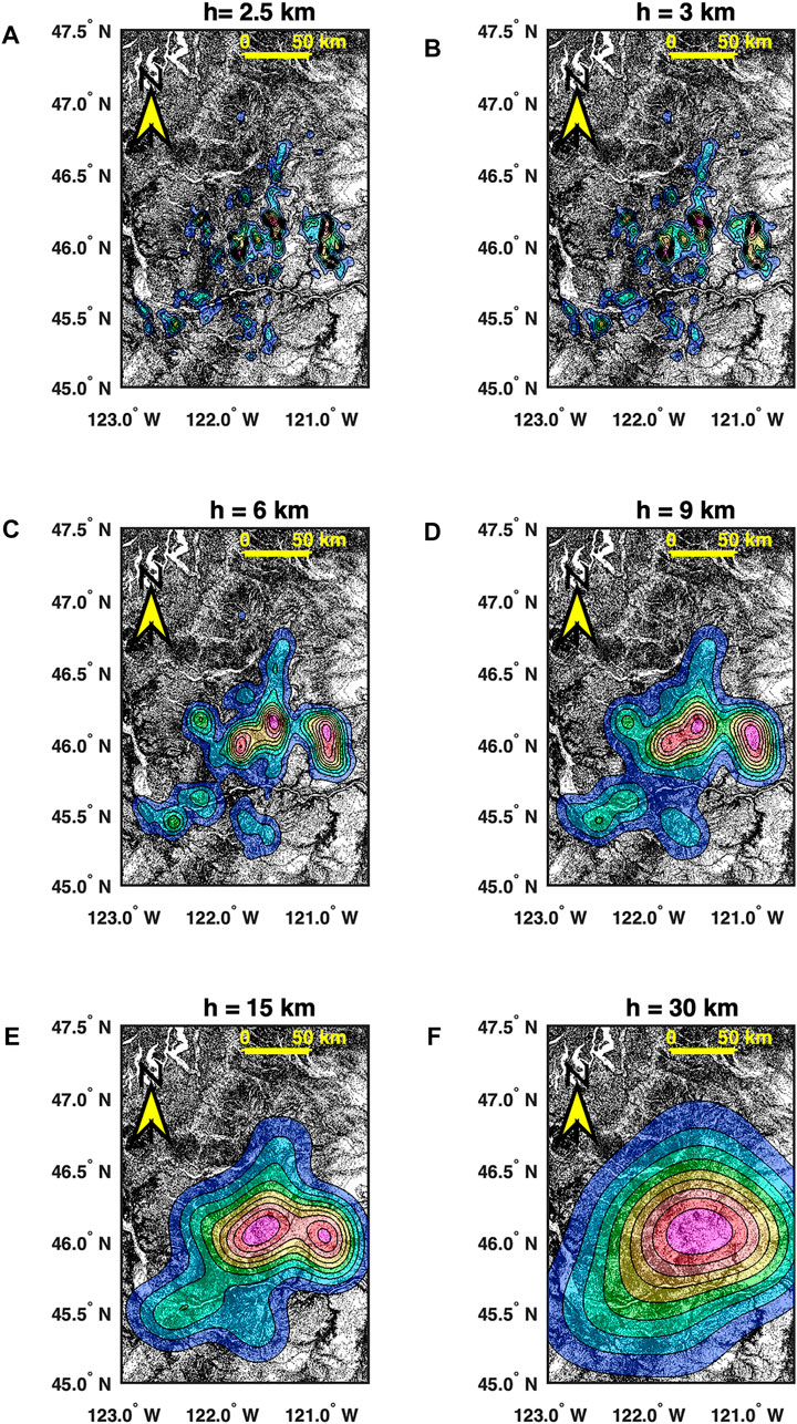
FIGURE 8. Sequence of PDFs used for exploration of the main features of the PDFs associated with the vent distribution of vents on the Washington Cascades.

As shown in Figure 6, the structure of the three main rifts, the central summit group and the areas where the SE Rift is complicated and intersected by other zones of linear volcanism are more clearly defined in the $\widehat{f}$ obtained with h = 0.5 (Figure 6A). The presence of the groups at the skirts of the main edifice are well defined in the $\widehat{f}$ s of h = 0.75 and 1 km (Figures 6B,C, respectively). h = 2 km and h = 6 km (Figures 6E,F) emphasize the nearly circular distribution of all of the vents, coinciding in a horizontal dimension almost perfectly with the outskirts of the main edifice. Similarly, in Figure 7 the sequence of $\widehat{f}$ s shown includes the “optimal” range, extending it a little to either larger and smaller hs than allowed with the predefined selectors. While the larger end emphasizes the spurious ellipsoid with a NE-SW orientation (Figure 7F), the whole progression of diagrams allows to identify such feature as a possible artifact of the form in which the various $\widehat{f}$ s are calculated (i.e., an artifact of the method of study), because it allows to see the progression between the several maxima as they appear or are split. Also, the smaller h shown (Figure 7A) reinforces the independence of several of the groups; independence that can be confirmed to be related to the presence of sills as identified in the field. Finally, for the case of the Washington Cascades, the sequence of $\widehat{f}$ s again extends the range of “optimal” h on both ends. The larger values of h (Figures 7E,F) reveal spurious $\widehat{f}$ s that nonetheless become suspect of being an artifact of the method when the complete sequence of $\widehat{f}$ s is examined because of the form in which the maxima are split over that sequence (jumping from one location to another). At the other extreme, the smaller values of h (Figures 7A,B) help to identify three main zones in an East-West direction on the maps, passing from an independent Simcoe Mountains group to a clearly elongated N-S array and a more diffuse set of groups to the west, some of which also seem to have a predominantly N-S orientation.

Thus, Figures 6–8 show three important facts: 1) the range of “optimal” h’s (i.e., those defined by using one of the “objective” selectors”) not always captures the entire set of interesting features of a region, but a wider range does, 2) the examination of the sequence of produced $\widehat{f}$ s allows identification of some of the spurious associations by establishing that some orientations might be more an artifact of the combination of two neighboring groups, each having a distinctive orientation that does not correspond to the orientation of the $\widehat{f}$ that yields a unique maximum that combines them, 3) examination of the sequence helps to reveal some details that are otherwise lost when only one $\widehat{f}$ is examined.

5.3 Is the Volcanic Case Very Special in Nature?

The results reported above illustrate that there is no “golden rule” to select one specific value of h. The existence of alternative statistic or probabilistic formulations making impossible the selection of just one model is not unique to the specific case of the KDE method examined in this work, but it is a common feature in many natural sciences. This has led to different approaches to deal with the uncertainty associated with the different models, and even has been referred to as the “range of technically defensible interpretations” (Ake et al., 2018) or the “extended expert’s distribution” (Marzocchi and Jordan, 2014). Furthermore, the different forms in which the existing information needs to be approached is at the heart of the general discussion that exists between the frequentist and Bayesian approaches and the different types in which various workers classify and handle different sources of error (Friedl and Hörmann, 2008; Marzocchi et al., 2021; O'Hagan, 2008). Thus, the specific problem of bandwidth selection with the kernel method is not exclusive of the volcanic context explored in this paper, but forms part of a wider context within the fields of probability and statistics. As it will be discussed next, which of those perspectives is adopted exerts some influence on the interpretations of results.

5.3.1 Probabilistic vs. Statistic Approach to Vent Distribution

From the perspective of hazard analysis (probabilistic in nature) it may not be important to know which of the existing systems in a region are those active at present, and depending on the information available it might be possible to focus attention on only a single PDF arising from a mixture of several processes. Nevertheless, if the objective of the study aims to infer clues concerning the physical structure present beneath a zone of distributed volcanism (statistic in nature), it might be more informative to examine the whole sequence of PDFs rather than trying to extract information only from one of those diagrams. In particular, it must be noted that the sequence of diagrams produced with increasing values of h follows an order that ultimately is controlled by the underlying structure. Such order is not random, and it is directly related to the specific situation that is under examination. In other words, the whole sequence of $\widehat{f}$ does not allow the analyst to “see what the analyst want to see” because the patterns that can be inferred from each sequence would not justify conclusions that belong to any of the other cases. For example, it is not possible to consider the existence of three rift zones joined in the centre of one system in neither the San Rafael or Washington cases, and it is also unjustified to identify a unique linear array in either the Mauna Kea and San Rafael cases. Consequently, even if it is possible that some subjective judgement could enter the interpretation of a sequence of $\widehat{f}$ s, those subjective assessments are unlikely to lead to wild guesses. At worst, they could lead to educated guesses that can be considered as hypothesis worth exploring either by including other already available sources of information or as a justification to prepare a grant request to obtain those additional sources. Indeed, some of those hypotheses might prove to be wrong when the additional information becomes available, but at least on those cases that particular hypothesis would have been tested.

On the other hand, if one encounters a situation in which only one $\widehat{f}$ is considered as valid, and such $\widehat{f}$ turns out to convey some misleading information, then not only the possibility of testing alternative hypotheses would have been lost, but also the beginning of the enthronement of wrong hypotheses would have been initiated. As shown by the examples of the San Rafael and Washington areas, some of the “optimal” estimators might lead to situations like this.

5.4 The Role of Experts’ Judgment

Another criticism that has been made to the exploration of several $\widehat{f}$ s is that relying on expert judgement to choose the appropriate h is a dated approach. This appreciation of the method is irrelevant because old approaches or methods are not necessarily incorrect or obsolete. Should this be the case, calculus would be entirely obsolete because it was developed by Leibniz and Newton around 300 years ago. Similarly, conclusions reached on the basis of the exploration of several $\widehat{f}$ s are often criticized and rejected on the basis of a lack of “objectivity”. Several forms to deal with those issues have been discussed in the context of forecasting natural hazards by Aspinall and Cooke (2013). Here I examine those issues to the light of a more general issue.

The convenience of learning to work with multiple hypothesis was formalized more than 100 years ago by Chamberlin (1897). As explained by Chamberlin, learning to work with multiple hypothesis promotes less inclination to misapply evidence and to more caution in drawing conclusions. The validity of that assertion is such that those ideas were reprinted half a century after they were first issued (Chamberlin, 1965), and it might be worth reprinting them once again to remind the new generations of scientists that attachment to a ruling theory not always is the best approach. Consequently, in line with the approach of multiple hypothesis, it is considered here that a thorough examination of a range of possible $\widehat{f}$ s is preferable to the commitment to only one of those estimates based in a selection of a method that might not even be applicable to the case under examination.

It is worth emphasizing that in the particular case of the analysis of spatial distributions of vents it is not suggested that each and every $\widehat{f}$ produced should be considered as an alternative hypothesis. This possibility not only would require the examination of an impossibly large number of diagrams, each produced with minute variations of h, but it also would imply that each $\widehat{f}$ is independent from the others. As shown by the examples of the three locations examined above, the interest on the examination of a sequence of $\widehat{f}$ s is not so much oriented to isolate and select only one of those diagrams. On the contrary, the main interest resides in the role that such an examination plays as an aid to appreciate the relationship that exists between the different maxima as h progresses. Indeed, some $\widehat{f}$ s may display some features more clearly than others, but it is also possible than different features of the system are highlighted at different values of h. Thus, the examination of a sequence of diagrams might lead to the selection of more than one $\widehat{f}$, each serving as the basis to formulate specific hypotheses about the distribution; hypotheses that might apply to different parts of the same region or involve different scales of observation, but that nonetheless might be related to a single volcanic system. The power of the method therefore resides not so much on its confirmatory character, but on its ability to provide a structured approach upon which different scales and possibilities can be assessed. Actually, it is such variety of information that might feed the expert’s opinion concerning which hypothesis are worth pursuing in a given region.

6 Concluding Remarks

As pointed out by Chamberlin (1965) investigations often proceed on the presumption that there is a definite process through which all results are of maximum excellence, and therefore the question of ‘what is the best method?’ is more often asked than ‘what are the special values of different methods, and what are their several advantageous applicabilities?‘. This frame of mind clearly promotes the point of view that problems often arise when assessment teams do not understand how to execute a specific method, when in reality there might not be errors, but only differences in opinion about the outcomes of different methods. Furthermore, in many cases it is implicitly assumed that the selected method of study is well conceived for the purposes of a specific application, which as shown in section 2, may not be always the case for KDE in many volcanic contexts. Nevertheless, as shown by the examples of section 4, the examination of a sequence of PDFs can provide enough clues to assess which of the conceptual situations depicted in Figure 1 seems better suited to describe a particular situation, or at least can be used to formulate better informed hypothesis that can be used to guide future studies in a region.

This approach has been well recognized in the context of inferential analysis on some branches of Earth sciences (e. g., Budnitz et al., 1997), but is not commonly appreciated in the context of statistical applications.

Thus, in parallel to this conceptual issue, throughout this work it has been shown that there is a large diversity of “unbiased” and/or “objective” estimators that can be used to select a single value of h that in turn can be used to produce a single estimator of the real PDF associated with a group of vents within a mainly statistical approach in mind. Because the real distribution of vents is a priori unknown, the range of “optimal” hs is not well constrained. Because some methods of estimation of h work better with some types of distribution than others, and also because we ignore the real distribution when examining the location of vents, the only form to be thorough in our analysis is to use more than one method to estimate h. In so doing, we are not far from adopting the exploratory approach in which a range of hs is used to produce a sequence of $\widehat{f}$ s, all of which are considered of some relevance. Examination of the complete sequence commonly provides clues to assess some aspects as probably spurious. Additionally, examination of a sequence of $\widehat{f}$ s is the only form to be sure that an analysis is not limited by the assumptions inherent to a theoretical-statistical point of view that may not correspond to the particular geologic-tectonic-volcanic situation under examination. Although in many cases it is probable that limiting the analysis to only one value of h may not be misleading, it is impossible to be sure if that is the case because, after all, we do not know for certain the real distribution. Consequently, despite the intentions of the researcher, any study that is based in only one h obtained by resorting to only one method of estimation, runs the risk of not only missing important information, but also it may even yield misleading clues concerning the physical characteristics of the volcanic system under examination.

Data Availability Statement

The raw data supporting the conclusions of this article will be made available by the author, without undue reservation.

Author Contributions

EC-T design, data processing, interpretation, and manuscript writing.

Funding

This research was provided fund by CONACYT grant A1-S-23107.

Conflict of Interest

The author declares that the research was conducted in the absence of any commercial or financial relationships that could be construed as a potential conflict of interest.

Publisher’s Note

All claims expressed in this article are solely those of the authors and do not necessarily represent those of their affiliated organizations, or those of the publisher, the editors and the reviewers. Any product that may be evaluated in this article, or claim that may be made by its manufacturer, is not guaranteed or endorsed by the publisher.

Acknowledgments

I thank the comments of J. Selva and two reviewers that helped to improve the clarity of this work. I also thank the continuous negative anonymous comments made to several papers submitted for publication over the past 5 years because this work would otherwise had not been deemed necessary. Finally, I also thank the editors for handling this work with the required open-mind alluded by one of the reviewers during the revision process.

References

Ake, J., Munson, C., Stamatakos, J., Juckett, M., Coppersmith, K., and Bommer, J. (2018). Updated Implementation Guidelines for SSHAC Hazard Studies. US Nuclear Regulatory Commission.

Google Scholar

Aspinall, W. P., and Cooke, R. M. (2013). “Quantifying Scientific Uncertainty from Expert Judgement Elicitation,” in Risk and Uncertainty Assessment for Natural Hazards. Editors J. Rougier, S. Sparks, and L. Hill (Cambridge: Cambridge University Press), 64–99.

Google Scholar

Bebbington, M. S., and Cronin, S. J. (2011). Spatio-temporal hazard Estimation in the Auckland Volcanic Field, New Zealand, with a New Event-Order Model. Bull. Volcanol. 73, 55–72. doi:10.1007/s00445-010-0403-6

CrossRef Full Text | Google Scholar

Bebbington, M. S. (2013). Assessing Spatio-Temporal Eruption Forecasts in a Monogenetic Volcanic Field. J. Volc. Geoth. Res. 252, 14–28. doi:10.1016/j.jvolgeores.2012.11.010

CrossRef Full Text | Google Scholar

Bebbington, M. S. (2015). Spatio-volumetric hazard Estimation in the Auckland Volcanic Field. Bull. Volcanol. 77, 39. doi:10.1007/s00445-00015-00921-0044310.1007/s00445-015-0921-3

CrossRef Full Text | Google Scholar

Bernreuter, D., L., Savy, J., B., Mensing, R., W., and Chen, J., C. (1988). Seismic hazard Characterization of 69 Nuclear Plant Sites East of Rocky Mountains. Lawrence Livermore National Laboratory.

Google Scholar

Bevilacqua, A., Bursik, M., Patra, A., Bruce Pitman, E., Sangani, R., Kobs‐Nawotniak, S., et al. (2018). Late Quaternary Eruption Record and Probability of Future Volcanic Eruptions in the Long Valley Volcanic Region (CA, USA). J. Geophys. Res. Solid Earth 123, 5466–5494. doi:10.1029/2018jb015644

CrossRef Full Text | Google Scholar

Budnitz, R., J., Apostolakis, G., Boore, D., M., Cluff, L., S., Coppersmith, K., J., Cornell, C., et al. (1997). Recommendations for Probabilistic Seismic hazard Analysis: Guidance on Uncertainty and Use of Experts. Lawrence Livermore National Laboratory.

Google Scholar

Cañón-Tapia, E. (2020). Influence of Method Selection on Clustering Analyses of point-like Features: Examples from Three Zones of Distributed Volcanism. Geomorphology 354, 107063. doi:10.1016/j.geomorph.2020.107063

CrossRef Full Text | Google Scholar

Cañon-Tapia, E. (2014). Insights into the Dynamics of Planetary Interiors Obtained through the Study of Global Distribution of Volcanoes II: Tectonic Implications from Venus. J. Volcanology Geothermal Res. 281, 70–84. doi:10.1016/j.jvolgeores.2014.05.013

CrossRef Full Text | Google Scholar

Cañon-Tapia, E., and Mendoza-Borunda, R. (2014). Insights into the Dynamics of Planetary Interiors Obtained through the Study of Global Distribution of Volcanoes I: Empirical Calibration on Earth. J. Volcanology Geothermal Res. 281, 53–69. doi:10.1016/j.jvolgeores.2014.05.015

CrossRef Full Text | Google Scholar

Cañón-Tapia, E. (2016). Reappraisal of the Significance of Volcanic fields. J. Volcanology Geothermal Res. 310, 26–38. doi:10.1016/j.jvolgeores.2015.11.010

CrossRef Full Text | Google Scholar

Cañón-Tapia, E. (2021a). Vent Distribution and Sub-volcanic Systems: Myths, Fallacies, and Some Plausible Facts. Earth-Science Rev. 221, 103768. doi:10.1016/j.earscirev.2021.103768

CrossRef Full Text | Google Scholar

Cañón-Tapia, E. (2021b). Vent Distribution on Jeju Island, South Korea: Glimpses into the Subvolcanic System. J. Geophys. Res. Solid Earth 126, e2021JB022269.

Google Scholar

Cañón-Tapia, E. (2013). Volcano Clustering Determination: Bivariate Gauss vs. Fisher Kernels. J. Volcanology Geothermal Res. 258, 203–214. doi:10.1016/j.jvolgeores.2013.04.015

CrossRef Full Text | Google Scholar

Cañón-Tapia, E. (2021c). “Volcano Distribution and Tectonics: A Planetoidic Perspective,” in In the Footsteps of Warren B. Hamilton: New Ideas in Earth Science. Editors G. Foulger, D. M. Jurdy, C. A. Stein, L. C. Hamilton, K. Howardet al. (Geological Society of America).

Google Scholar

Chamberlin, T. C. (1897). Studies for Students: The Method of Multiple Working Hypotheses. J. Geology. 5, 837–848. doi:10.1086/607980

CrossRef Full Text | Google Scholar

Chamberlin, T. C. (1965). The Method of Multiple Working Hypotheses. Science 148, 754–759. doi:10.1126/science.148.3671.754

PubMed Abstract | CrossRef Full Text | Google Scholar

Champion, D. E., Cyr, A., Fierstein, J., and Hildreth, W. (2018). Monogenetic Origin of Ubehebe Crater Maar Volcano, Death Valley, California: Paleomagnetic and Stratigraphic Evidence. J. Volcanology Geothermal Res. 354, 67–73. doi:10.1016/j.jvolgeores.2017.12.018

CrossRef Full Text | Google Scholar

Condit, C. D., and Connor, C. B. (1996). Recurrence Rates of Volcanism in Basaltic Volcanic fields: An Example from the Springerville Volcanic Field, Arizona. Geol. Soc. Am. Bull. 108, 1225–1241. doi:10.1130/0016-7606(1996)108<1225:rrovib>2.3.co;2

CrossRef Full Text | Google Scholar

Connor, C. B. (1987). Cinder Cone Distribution Described Using Cluster Analysis and Two-Dimensional Fourier Analysis in the Central Transmexican Volcanic Belt, Mexico, and in SE Guatemala and NW El Salvador. Hanover: Darmouth College, 318.

Google Scholar

Connor, C. B., Connor, L., Germa, A., Richardson, J., Bebbington, M., Gallant, E., et al. (2019). How to Use Kernel Density Estimation as a Diagnostic and Forecasting Tool for Distributed Volcanic Vents. Siv 43, 1–25. doi:10.5038/2163-338x.4.3

CrossRef Full Text | Google Scholar

Connor, C. B., and Connor, L. J. (2009). “Estimating Spatial Density with Kernel Methods,” in Volcanic and Tectonic hazard Assessment for Nuclear Facilities. Editors C. B. Connor, N. A. Chapman, and L. J. Connor (Cambridge: Cambridge University Press), 346–368.

Google Scholar

Connor, C., and Hill, B. E. (1995). Three Nonhomogeneous Poisson Models for the Probability of Basaltic Volcanism: Application to the Yucca Mountain Region. J. Geophys. Res. 100, 107–125. doi:10.1029/95jb01055

CrossRef Full Text | Google Scholar

Conway, F. M., Connor, C. B., Hill, B. E., Condit, C. D., Mullaney, K., and Hall, C. M. (1998). Recurrence Rates of Basaltic Volcanism in SP Cluster, San Francisco Volcanic Field, Arizona. Geol 26, 655–658. doi:10.1130/0091-7613(1998)026<0655:rrobvi>2.3.co;2

CrossRef Full Text | Google Scholar

DeGroot, M. H., and Schervish, M. J. (2012). Probability and Statistics. Boston: Addison-Wesley.

Google Scholar

Delcamp, A., Mossoux, S., Belkus, H., Tweheyo, C., Mattsson, H. B., and Kervyn, M. (2019). Control of the Stress Field and Rift Structures on the Distribution and Morphology of Explosive Volcanic Craters in the Manyara and Albertine Rifts. J. Afr. Earth Sci. 150, 566–583. doi:10.1016/j.jafrearsci.2018.09.012

CrossRef Full Text | Google Scholar

Duong, T., and Hazelton, M. (2003). Plug-in Bandwidth Matrices for Bivariate Kernel Density Estimation. J. Nonparametric Stat. 15, 17–30. doi:10.1080/10485250306039

CrossRef Full Text | Google Scholar

Duong, T. (2007). Ks: Kernel Density Estimation and Kernel Discriminant Analysis for Multivariate Data in R. J. Stat. Softw. 21. doi:10.18637/jss.v021.i07

CrossRef Full Text | Google Scholar

Frankel, A. (1995). Mapping Seismic Hazard in the Central and Eastern United States. Seismological Res. Lett. 66, 8–21. doi:10.1785/gssrl.66.4.8

CrossRef Full Text | Google Scholar

Friedl, H., and Hörmann, S. (2008). “Frequentist Probability Theory,” in Handbook of Probability. Editor T. Rudas (Los Angeles: SAGE Publications), 15–34.

Google Scholar

Heidenreich, N. B., Schindler, A., and Sperlich, S. (2013). Bandwidth Selection for Kernel Density Estimation: a Review of Fully Automatic Selectors. Asta Adv. Stat. Anal. 97, 403–433. doi:10.1007/s10182-013-0216-y

CrossRef Full Text | Google Scholar

Hiemer, S., Woessner, J., Basili, R., Danciu, L., Giardini, D., and Wiemer, S. (2014). A Smoothed Stochastic Earthquake Rate Model Considering Seismicity and Fault Moment Release for Europe. Geophys. J. Int. 198, 1159–1172. doi:10.1093/gji/ggu186

CrossRef Full Text | Google Scholar

Hildreth, W. (2007). Quaternary Magmatism in the Cascades - Geological Perspectives. US Geological Survey, 125.

Google Scholar

Jacobo-Bojórquez, R. A., and Cañón-Tapia, E. (2020). Distribution of Eruptive Centers on Top of Large Shield Volcanoes in the Inner Solar System: General Classification and Glimpses of Their Subvolcanic Structure. J. Geophys. Res. Planets 125, e2020JE006431.

Google Scholar

Jaquet, O., Connor, C., and Connor, L. (2008). Probabilistic Methodology for Long-Term Assessment of Volcanic Hazards. Nucl. Tech. 163, 180–189. doi:10.13182/nt08-a3980

CrossRef Full Text | Google Scholar

Jones, M. C., Marron, J. S., and Sheather, S. J. (1996). Progress in Data-Based Bandwidth Selection for Kernel Density Estimation. Comput. Stat. 11, 337–381.

Google Scholar

Jones, M. C. (1991). The Roles of ISE and MISE in Density Estimation. Stat. Probab. Lett. 12, 51–56. doi:10.1016/0167-7152(91)90163-l

CrossRef Full Text | Google Scholar

Kereszturi, G., and Németh, K. (2013). “Monogenetic Basaltic Volcanoes: Genetic Classification, Growth, Geomorphology and Degradation,” in Updates in Volcanol- Ogy: New Advances in Understanding Volcanic Systems. Editor K. Németh (InTech), 3–88.

Google Scholar

Kiyosugi, K., Connor, C. B., Ferwerda, B. P., Germa, A. M., Connor, L. J., Hintz, A. R., et al. (2012). Relationship between dike and Volcanic Conduit Distribution in a Highly Eroded Monogenetic Volcanic Field: San Rafael, Utah, USA. Geology 40, 695–698. doi:10.1130/g33074.1

CrossRef Full Text | Google Scholar

Kiyosugi, K., Connor, C. B., Zhao, D., Connor, L. J., and Tanaka, K. (2009). Relationships between Volcano Distribution, Crustal Structure, and P-Wave Tomography: an Example from the Abu Monogenetic Volcano Group, SW Japan. Bull. Volcanol. 72 (3), 331–340. doi:10.1007/s00445-009-0316-4

CrossRef Full Text | Google Scholar

Lutz, M. T., and Gutmann, J., T. (1995). An Improved Method for Determining and Characterizing Alignements of point like Features and its Implications for the Pinacate Volcanic Field, Sonora, Mexico. J. Geophys. Res. 100, 17 659–617 670. doi:10.1029/95jb01058

CrossRef Full Text | Google Scholar

Marzocchi, W., and Bebbington, M. S. (2012). Probabilistic Eruption Forecasting at Short and Long Time Scales. Bull. Volcanol. 74 (8), 1777–1805. doi:10.1007/s00445-012-0633-x

CrossRef Full Text | Google Scholar

Marzocchi, W., and Jordan, T. H. (2014). Testing for Ontological Errors in Probabilistic Forecasting Models of Natural Systems. Proc. Natl. Acad. Sci. U.S.A. 111, 11973–11978. doi:10.1073/pnas.1410183111

PubMed Abstract | CrossRef Full Text | Google Scholar

Marzocchi, W., Sandri, L., and Selva, J. (2008). BET_EF: a Probabilistic Tool for Long- and Short-Term Eruption Forecasting. Bull. Volcanol. 70, 623–632. doi:10.1007/s00445-007-0157-y

CrossRef Full Text | Google Scholar

Marzocchi, W., Selva, J., and Jordan, T. H. (2021). A Unified Probabilistic Framework for Volcanic hazard and Eruption Forecasting. Nat. Hazards Earth Syst. Sci. 21, 3509–3517. doi:10.5194/nhess-21-3509-2021

CrossRef Full Text | Google Scholar

Marzoli, A., Callegaro, S., Dal Corso, J., Davies, J. H. F. L., Youbi, N., Bertrand, H., et al. (2018). “The Central Atlantic Magmatic Province (CAMP): A Review,” in The Late Triassic World. Editor L. H. Tanner (Cham: Springer), 91–125. doi:10.1007/978-3-319-68009-5_4

CrossRef Full Text | Google Scholar

Németh, K., and Kereszturi, G. (2015). Monogenetic Volcanism: Personal Views and Discussion. Int. J. Earth Sci.. doi:10.007/s00531-015-1243-610.1007/s00531-015-1243-6

CrossRef Full Text | Google Scholar

Neri, A., Aspinall, W. P., Cioni, R., Bertagnini, A., Baxter, P. J., Zuccaro, G., et al. (2008). Developing an Event Tree for Probabilistic hazard and Risk Assessment at Vesuvius. J. Volcanology Geothermal Res. 178, 397–415. doi:10.1016/j.jvolgeores.2008.05.014

CrossRef Full Text | Google Scholar

O'Hagan, (2008). “The Bayesian Approach to Statistics,” in Handbook of Probability. Editor T. Rudas (Los Angeles: SAGE Publications), 85–100.

Google Scholar

Porter, S., C. (1972). Distribution, Morphology, and Size Frequency of Cinder Cones on Mauna Kea Volcano. Hawaii Bull. Geol. Soc. Am. 83, 3 607–603 612. doi:10.1130/0016-7606(1972)83[3607:dmasfo]2.0.co;2

CrossRef Full Text | Google Scholar

Richardson, J. A., Miller, D. M., Bleacher, J. E., Connor, C., Gregg, T. K., Connor, L., et al. (2012). Comparison of Monogenetic Volcano Clusters on Earth, Venus and Mars. San Francisco, CA: AGU Fall Meeting. abstract # V44C-04.

Google Scholar

Ripley, B. D. (1981). Spatial Statistics. USA: John Wiley & Sons.

Google Scholar

Rivalta, E., Corbi, F., Passarelli, L., Acocella, V., Davis, T., and Di Vito, M. A. (2019). Stress Inversions to Forecast Magma Pathways and Eruptive Vent Location. Sci. Adv. 5. doi:10.1126/sciadv.aau9784

PubMed Abstract | CrossRef Full Text | Google Scholar

Rose, W., I., Palma, J., L., Escobar Wolf, R., and Matías Gomez, R., O. (2013). “A 50 Yr Eruption of a Basaltic Composite Cone: Pacaya, Guatemala,” in Understanding Open-Vent Volcanism and Related Hazards. Editors W. Rose, I. J. Palma, H. Delgado-Granados, and N. R. Varley (Boulder: Geological Society of America), 1–21. doi:10.1130/2013.2498(01)

CrossRef Full Text | Google Scholar

Rosenblatt, M. (1956). Remarks on Some Nonparametric Estimates of a Density Function. Ann. Math. Stat. 27, 642–669. doi:10.1214/aoms/1177728190

CrossRef Full Text | Google Scholar

Schindler, A. (2011). Bandwidth Selection in Nonparametric Kernel Estimation. Georg-August-Universitat.

Google Scholar

Scott, D. W. (1992). Multivariate Density Estimation: Theory, Practice, and Visualization. New york: Wiley, 317.

Google Scholar

Selva, J., Acocella, V., Bisson, M., Caliro, S., Costa, A., Della Seta, M., et al. (2019). Multiple Natural Hazards at Volcanic Islands: a Review for the Ischia Volcano (Italy). J. Appl. Volcanol. 8, 5. doi:10.1186/s13617-019-0086-4

CrossRef Full Text | Google Scholar

Sheather, S. J., and Jones, M. C. (1991). A Reliable Data-Based Bandwidth Selection Method for Kernel Density Estimation. J. R. Stat. Soc. Ser. B (Methodological) 53, 683–690. doi:10.1111/j.2517-6161.1991.tb01857.x

CrossRef Full Text | Google Scholar

Silverman, B. W. (1986). Density Estimation for Statistics and Data Analysis. New York: Chapman & Hall, 175.

Google Scholar

Silverman, B. W. (1981). Using Kernel Density Estimates to Investigate Multimodality. J. R. Stat. Soc. Ser. B (Methodological) 43, 97–99. doi:10.1111/j.2517-6161.1981.tb01155.x

CrossRef Full Text | Google Scholar

Skiena, S. (2003). Calculated Bets. Computers, Gambling, and Mathematical Modeling to Win. Cambridge UK: Cambridge University Press, 232.

Google Scholar

Srisutthiyakorn, N., Kiefer, W. S., and Kirchoff, M. (2010). Spatial Distribution of Volcanoes in the Marius Hills and Comparison with Volcanic fields on Earth and Venus. Lunar Planet. Sci. Conf. 41. abstract 1185.

Google Scholar

Stock, M. J., Bagnardi, M., Neave, D. A., Maclennan, J., Bernard, B., Buisman, I., et al. (2018). Integrated Petrological and Geophysical Constraints on Magma System Architecture in the Western Galápagos Archipelago: Insights from Wolf Volcano. Geochem. Geophys. Geosyst. 19, 4722–4743. doi:10.1029/2018gc007936

CrossRef Full Text | Google Scholar

Szakács, A., and Cañón-Tapia, E. (2010). “Some Challenging New Perspectives of Volcanology,” in What Is a Volcano? Editors E. Cañón-Tapia, and A. Szakács (Geological Society of America), 123–140. doi:10.1130/2010.2470(09)

CrossRef Full Text | Google Scholar

Turlach, B. A. (1993). Bandwidth Selection in Kernel Density Estimation: A Review. Humbolt-Universitat zu Berlin. Discussion Paper 9307 Institut fur Statistik und Okonometrie.

Google Scholar

Valentine, G. A., and Gregg, T. K. P. (2008). Continental Basaltic Volcanoes - Processes and Problems. J. Volcanology Geothermal Res. 177, 857–873. doi:10.1016/j.jvolgeores.2008.01.050

CrossRef Full Text | Google Scholar

Wand, M. P., and Jones, M. C. (1994). Multivariate Plug-In Bandwidth Selection. Comput. Stat. 9, 97–116.

Google Scholar

Wand, M. P., and Jones, M. C. (1993). Comparison of Smoothing Parameterizations in Bivariate Kernel Density Estimation. J. Am. Stat. Assoc. 88, 520–528. doi:10.1080/01621459.1993.10476303

CrossRef Full Text | Google Scholar

Weller, J. N., Martin, A. J., Connor, C. B., Connor, L. J., and Karakhanian, A. (2006). “Modelling the Spatial Distribution of Volcanoes: an Example from Armenia,” in Statistics in Volcanology. Editors H. Mader, M. S. Coles, C. Connor, and L. J. Connor (London: Geological Society), 77–87.

Google Scholar

Wolfe, E., W., Wise, W., S., and Dalrymple, G., B. (1997). The Geology and Petrology of Mauna Kea Volcano, Hawaii - A Study of Postshield Volcanism. U.S. Geol. Surv.. doi:10.3133/pp1557

CrossRef Full Text | Google Scholar