Advances and Accuracy Assessment of Ocean Tide Models in the Antarctic Ocean

Ocean tides in polar regions play an important role in the study of sea ice dynamics and floating ice shelves. The accuracy of existing ocean tide models in shallow waters and polar seas is much lower than that in open deep oceans. This study summarized the advances of state-of-the-art global tide models in the Antarctic Ocean, the construction of tide models around Circum-Antarctica, and five typical regions: Antarctic Peninsula, Ross Sea, Filchner–Ronne Ice Shelf (FRIS), Weddell Sea, and Amery Ice Shelf (AIS). The accuracy of FES 2014, TPXO9, EOT20, CATS 2008, and regional tide models in the Antarctic Ocean and typical areas was evaluated using tidal records and satellite altimetry data. EOT20 and ANTPEN04.01 models have higher accuracy in the Antarctic Peninsula, and the root sum square (RSS) values are 8.29 and 7.46 cm, respectively. TPXO9 has the highest accuracy in the Weddell Sea and FRIS and AIS and RSS values are 18.33 and 12.77 cm, respectively. TPXO9 and RIS_Optimal models have higher accuracy in the Ross Sea and Ross Ice Shelf (RIS), RSS values are 5.62 and 6.21 cm, respectively. The accuracy of FES 2014, TPXO9, CATS 2008, and the regional tide model in the Drake Passage, Kerguelen Islands, and Adelie–Mertz was evaluated using satellite altimetry data. The RSS values are less than 4 cm. By using the altimetry data at Sentinel-3A single-satellite crossovers in terms of the STD of the SLA, the comparison of the STDs show that FES2014 is the best.

1 Introduction

Ocean tides are the main source of high-frequency variability in the vertical and horizontal motion of ice sheets near their marine margins. Lateral motion of floating and grounded portions of ice sheets near their marine margins can also include a tidal component. Tide height ranges can change substantially as ice sheets change their thickness and extent. The ocean tide is also the main source of high-frequency “noise” in satellite-based measurements that are used to monitor long-term changes in the ocean and marine cryosphere. Accurate tidal measurements and forecasts are necessary for the study in the tide and icesheet interaction and for satellite altimeter data correction. In recent years, due to the wide application of satellite altimetry data, great progress has been made in the construction of the global tide model.

The performance of tide models varies from region to region and from constituent to constituent. Due to a series of reasons, the accuracy of tide models in the Arctic Ocean and around Antarctica is always lower than that in other regions, and there is regional variability within the polar tide models. For example, it exceeds the coverage of TOPEX/Poseidon (T/P) series satellites and lacks high-precision altimetry data. The seasonal variation of sea ice and the existence of large ice shelves seriously hinder the satellite altimeter to measure sea level height. At the same time, due to the harsh climatic environment in the polar seas, the measured data resources such as tide stations around are also relatively scarce. Therefore, there is lack of data for modeling or constraining the ocean tides in polar seas, and the consistency among different models is weak.

King and Padman (2005) evaluated the accuracy of six global tide models (FES 2004, TPXO7.2, etc.) and two Antarctic tide models (CADA00.10 and CATS02.01) around the Antarctic Ocean using tide gage, gravimeter, and GPS data. The optimal model for the whole Antarctic Ocean is TPXO6.2. King et al. (2005) evaluated the accuracy of the tide model based on tidal load and GPS data. Using 102 tide records, Stammer et al. (2014) evaluated the accuracy of six global tide models, such as FES2012 and TPXO8. In the Antarctic Ocean, TPXO8 has the highest accuracy. Lei et al. (2017) evaluated the accuracy of eight global tide models in the Antarctic Ocean but did not analyze the accuracy of the Circum-Antarctic tide models and typical regional tide models. Shepherd and Peacock verified the tide models around the Antarctic Peninsula. Oreiro et al. (2014) evaluated the accuracy of eight global tide models, including GOT4.7, and four regional tide models, including CADA00.10, in the Antarctic Peninsula using satellite altimetry data and tide gage data. Padman and Erofeeva (2005) evaluated the tide observed using ICESat in the Ross Ice Shelf (RIS). Kim et al. (2011) evaluated the accuracy of tide models at the Syowa station using superconducting gravity data, and the results show that TPXO7.2 has the highest accuracy.

Since previous studies have not integrated the global tide models and the Antarctic regional tide for evaluation, this study will focus on the research work of global tide models in the Antarctic Ocean, the construction of tide models around the Antarctic Ocean and typical regions in Antarctica, and evaluate the accuracy of tide models in the Circum-Antarctic Ocean and typical sea areas. The remainder of the study is structured as follows in section 2, we briefly summarize most of the modern global tide models, Antarctic tide models, and regional tide models in Antarctica. Section 3 presents the datasets and methodology used to assess the accuracy of CATS 2008, FES 2014, TPXO9, EOT20, and several regional models. Section 4 presents the results of the intercomparisons among CATS 2008, FES2014, TPXO9, and EOT20 and evaluates the models against in situ data and satellite altimetry data. Conclusions are provided in section 5.

2 Research Progress of Tide Models

At present, the construction methods of tide models mainly include the empirical model, hydrodynamic model, and assimilation model based on hydrodynamic equations and measured data. The following is a brief overview of the global tide models (including four empirical models and five assimilation models), the Circum-Antarctic tide models (including three hydrodynamic models and two assimilation models), and the typical regional tide models in Antarctica. In this study, only the latest tide models in each series are described.

The key features of the state-of-the-art models are listed in Table 1. Regional models listed in Table 1 can be used by Tide Model Driver (Padman and Erofeeva, 2005).

TABLE 1

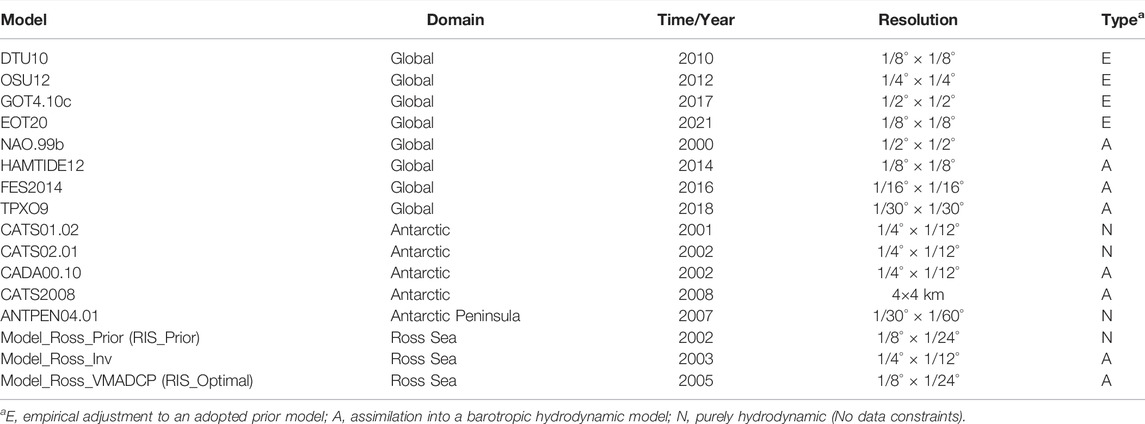
TABLE 1. Summary of ocean tide models.

2.1 Modern Global Tide Models

The empirical models include the Technical University of Denmark (DTU) series models, Ohio State University (OSU), Goddard Ocean Tide (GOT) series models, and Empirical Ocean Tide (EOT) series models. DTU (Cheng and Andersen, 2011) series models were established by the Technical University of Denmark. DTU10 is the latest released model, beyond latitude ±66°; the DTU10 model combines ERS-2, GFO, and Envisat altimetry data to improve the quality of observations using the unit method and applies the hybrid altimetry-hydrological model DTU10ANN to remove the annual influence of sea-level changes before estimating the residual water level to improve the accuracy of diurnal constituent tide measurement of the sun-synchronous satellite (ERS-2, Envisat) in the polar region. The OSU12 (Fok, 2012) model was built by the United States Ohio State University. OSU12 directly uses the results of the GOT4.7 tide model in the sea area beyond latitude ±66°, and the results are interpolated into 1/4°. The GOT (Ray, 1999; Ray, 2013) series models were developed by the United States Goddard Space Flight Center (GSFC). GOT4.10c is the updated GOT99 model implemented based on an empirical harmonic analysis of a satellite altimeter. Unlike its predecessors, for example, 4.7, 4.8, and 4.9 in GOT4.10c, Jason-1, and Jason-2 have been, respectively, used without considering T/P data. In shallow waters and deepwater poleward of 66°, data from Geosat Follow-On, ERS-1, and ERS-2 were used. A small amount of early ICESat data was used in the Weddell and Ross seas. GOT4.10c has the coarsest spatial resolution of 1/2°, and it is, therefore, expected to be less accurate in near-coastal water. The EOT (Savcenko and Bosch, 2012; Hart-Davis et al., 2021) series models were built by Germany Deutsches Geoditisches Forschungs Institut. The latest EOT series model is EOT20. EOT20 (Hart-Davis et al., 2021) uses altimetry data for 26 years from 1992 to 2018, including T/P, Jason-1/2, ERS-2, and Envisat satellites, with a grid resolution of 1/8°. Compared with EOT11a and EOT19, the EOT20 model shows significant improvements, particularly in the coastal and shelf regions, and due to the inclusion of more recent satellite altimetry data and more missions, the use of the updated FES2014 tide model is taken as a reference to estimated residual signals.

Assimilation models are widely used with high accuracy, including National Astronomical Observatory version 99b (NAO.99b), HAMTIDE series models, FES series model, and TPXO series models. NAO.99b (Matsumoto et al., 2000) is established by the National Astronomical Observatory of Japan. NAO.99b has assimilated five years of T/P satellite altimeter along-track data using the “blending” assimilation method, and the grid resolution is 1/2°. HAMTIDE series models (Taguchi et al., 2014) are established by the University of Hamburg in Germany. HAMTIDE series tide models have assimilated the time series of T/P and Jason-1 for 15 years, and the grid resolution is 1/8°. HAMTIDE12 is the latest model and is based on the linearized tidal hydrodynamic equations and on a simple harmonic time dependence of the variables. Finite difference methods were adopted for numerically solving the equations. EOT11a output was used between 74°N and 84°S as a constraint. FES series tide models (Lefevre et al., 2002; Lyard et al., 2006; Carrère et al., 2012; Carrère et al., 2016; Lyard et al., 2020) are developed by the French Tidal Group. The FES2014 model (Carrère et al., 2016; Lyard et al., 2020) is the latest model based on the tidal barotropic equation of spectral structure; it has assimilated the time series of T/P, Jason-1/2, ERS-1/2, and Envisat satellites for 20 years corrected by a new geophysical model using Spectral Ensemble Optimal Interpolation assimilation software, and the grid resolution is 1/8°. The accuracy of FES2014 is greatly improved in shallow waters and polar regions. TPXO series models (Egbert and Ray, 2000; Egbert and Erofeeva, 2002; Egbert et al., 2018) were established by Oregon State University in the United States. TPXO8 adds ERS, Envisat, and tide gage data in the polar region, and the grid resolution is 1/30°. TPXO9 (Egbert et al., 2018) is the latest version of TPXO series tide models, which has updated the water depth data and satellite altimetry data.

2.2 Circum-Antarctic Tide Models

The hydrodynamic models include the CATS01.02 (Circum-Antarctic Tidal Simulation) tide model and CATS02.01 tide model, which were constructed by Laurie Padman in Earth and Space Research and Helen Amanda Fricker in the University of California San Diego. The CATS01.02 (Circum-Antarctic Tidal Simulation) model (Padman and Kottmeier, 2000; Padman et al., 2002) is a regional finite-difference model, which is solved using a standard quadratic function. The resolution is 1/4° × 1/12° (longitude × latitude), the coverage is the whole Antarctic Ocean to the south of 50°S, and the northern open boundary was constrained using the FES95 model. The CATS02.01 tide model (Padman et al., 2002) is a tide model around the Antarctic Ocean based on a shallow water dynamic equation. CATS02.01 is solved using a linear friction equation. It is the best fitting to the tide height and current of the Ross Sea. The resolution is 1/4° × 1/12° (longitude × latitude). CATS02.01 is driven by TPXO5.1 sea surface heights along the northern open boundary.

Assimilation models are also constructed by Laurie Padman and Helen Amanda Fricker et al., including the tide models of CADA00.10 and CATS 2008. The CADA00.10 (Circum-Antarctic Data Assimilation) tide model (Padman et al., 2002) covers the Antarctic Ocean to the south of 58°S, with a spatial resolution of 1/4° × 1/12° (longitude × latitude). The CATS00.10 model is driven by time-stepping TPXO5.1-derived sea surface height along the northern open boundary at 58°S. It has assimilated the data of 25 tide stations in Antarctica and 270 T/P satellite points (north of 66.2°S). The CATS2008 tide model (Padman et al., 2008) is a high-resolution tide model with a spatial resolution of 4 km. It was forced from the global inverse model TPXO7.1 at the northern open boundary. The data assimilated by the model include T/P satellite altimetry data when no sea ice is present; 50 high-quality tide records (including sea bottom pressure data, tide station data, and part of GPS data) and the ICESat altimetry data at crossovers in the RIS and Filchner–Ronne Ice Shelf (FRIS).

2.3 Antarctic Regional Tide Models

ANTPEN04.01 (Oreiro et al., 2014) (AntPen, for short) is a regional hydrodynamic model for the entire Antarctic Peninsula with a spatial resolution of 1/30° × 1/60° (longitude × latitude). The model domain includes ocean cavities under the floating ice shelves and is based on linearized shallow-water equations forced at the open boundary by tide heights from the Circum-Antarctic forward model (CATS02.01) and astronomical forcing. The model inverses eight main tide constituents, including four semidiurnal constituents and four diurnal constituents.

The ocean tides in the Ross Sea have been an active area of research. Padman et al. (2008) constructed the assimilation Model_Ross_Inv in 2003; the coverage area of the model is 63°S∼86°S, 150°E∼220°E. The model spatial resolution is 1/4° × 1/12° (longitude × latitude), and it used TPXO5.1 under conditions of the open boundary. The assimilation data include T/P altimetry data to the north of 66°S and 10 datasets of tide gage and gravimeter on the RIS. Some scholars have built a hydrodynamic Model_Ross_Prior (RIS_Prior) (Padman et al., 2003; Padman et al., 2008) in the Ross Sea; the coverage area of the model is 63°S∼86°S, 159°E∼215°E. The model resolution is 1/8° × 1/24° (longitude × latitude), and it used CATS02.01 under conditions of the open boundary. Based on the aforementioned hydrodynamic model, Erofeeva et al. (2005) constructed the Model_Ross_VMADCP (RIS_Optimal), which uses TPXO5.1 under conditions of open boundary, and three sets of ADCP data are assimilated at the north boundary.

Smithson et al. (1996) simulated the tides in the Filchner–Ronne Ice Shelf region. The study area covers 60°S∼85°S, 90°W∼10°W, and the model resolution is 40′× 10′. Because it includes a permanent ice layer, the model uses water column data rather than water depth data. Along the open boundary, time series of sea surface heights for each node was used to force the model. Tide height coefficients were obtained from the Schwiderski global ocean tide model.

Robertson et al. (1998) studied the tides in the Weddell Sea and built a tide model. The model domain is 55°S∼83°S and 84°W∼10°E. The water depth data comes from the global water depth data model ETOPO-5. The model simulated four tide constituents of M2, S2, O1, and K1. At open boundaries, tide-height coefficients obtained from TPXO3 were used.

Hemer et al. (2006) studied the tide model in the Amery Ice Shelf (AIS). The modeling area covers the AIS and Prydz Bay, extending to the continental shelf slope. The depth data of Prydz Bay on the north side of the ice field are combined with ship track data and BEDMAP data. The CADA00.10 model is adopted under conditions of open boundary, which assimilates the tide data of Davis and Mawson stations in Prydz Bay.

3 Data and Methodology Used for the Estimation of Tide Models

3.1 Data Records

We use 86 tide stations to the south of 55°S. The data sources include 28 bottom pressure recorders (BPR), seven coastal tide gages, 25 GPS stations, 12 gravimeters, two tilt instruments, four moored pressure tide gages, and eight visual tide staffs (Figure 1). The highest-quality data come from BPR, coastal tide gages, and GPS records. Most of those data records are longer than 1/2 years, and the major tidal constituents can be best separated. Many Antarctic records are less than 29 days long so that they are difficult to analyze for a sufficient number of major tides to develop reliable predictive models for that site. Nevertheless, because few tide records exist around Antarctica, these shorter records (the intermediate-length records between 29 days and 1/2 years long) are also valuable to users. The tide constituents of all stations, as well as information on record length, measurement type, and references, can be found in the Antarctic tide survey database. The data records of the gravimeter and tiltmeter are short and older without strict data correction, which are considered to be unreliable. Gravimeter records account for a large part of RIS records. Tide gages usually have quality control. BPR measurements are mainly distributed near the Antarctic Peninsula, and GPS measurements are mainly distributed near the Weddell Sea and Ross Sea. The gravimeter and tiltmeter are mainly distributed in RIS and FRIS.

FIGURE 1

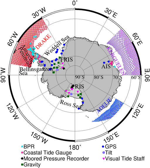
FIGURE 1. Locations of all tidal measurements and X-Track satellite altimetry track coverage.

The Center for Topographic Studies in the Sea and Hydrosphere (CTOH) computes eight main tidal constants (including M2, S2, N2, K2, K1, O1, P1, and Q1) estimated from its along-track 1Hz sea level anomaly (SLA) products. Taking advantage of the long time series of altimetry data, the regional CTOH sea level anomaly database has been harmonically analyzed to derive empirical tidal constituents, every 6–7 km along the satellite ground tracks (Roblou et al., 2011). These datasets are distributed by Archiving, Validation, and Interpretation of Satellite Oceanographic (AVISO). X-Track provides harmonic constants for three regions in the Antarctic Ocean, including the Drake Passage, Kerguelen Islands, and Adelie–Mertz (Figure 1). The data for harmonic analysis were taken from the T/P and Jason satellite altimeters. The data of the original orbit include T/P, Jason-1, and Jason-2, spanning the period from 28th February 1992 (cycle 17 of T/P) to 24th July 2015 (cycle 259 of Jason-2). The data of the interleaved orbit include T/P and Jason-1, spanning the period from 21st September 2002 (cycle 369 of T/P) to 2nd February 2012 (cycle 372 of Jason-1).

3.2 Comparison Method of Tide Models Against Tide Gages and Satellite Altimetry

To quantify each tidal constituent error between observation results and tide models, the root mean square (RMS) misfits were calculated using the following equations (Lei et al., 2017):

$RMS={\left\{\frac{1}{N}{\displaystyle \sum _{i=1}^N\frac{1}{2}\left[{\left(H_n\cos \left(G_n\right)-H_m\cos \left(G_m\right)\right)}^2+{\left(H_n\sin \left(G_n\right)-H_m\sin \left(G_m\right)\right)}^2\right]}\right\}}^{\frac{1}{2}},(1)$

where $H_n,G_n$ are the amplitude and Greenwich phase of a constituent given by observation data and $H_m,G_m$ are the corresponding amplitude and Greenwich phase of a constituent given by tide models. N is the number of observation points.

In addition, to assess the performance of each model, the root sum square (RSS) was calculated using Eq. 2.

$RSS={\left({\displaystyle \sum _{j=1}^{J}RM{S}_j^2}\right)}^{\frac{1}{2}},(2)$

where $J$ is the total number of constituents.

4 Evaluation of Tide Models

With the improvement of spatial resolution and increase of assimilation data, the accuracy of the new models has been improved compared with the earlier models. Stammer et al. (2014) has concluded that TPXO8 is the most accurate model around Antarctica, so in the subsequent comparison, only global tidal models built after 2014 are compared. Due to the lowest resolution of the GOT4.10c, it is not compared in this study. Therefore, in the following analysis, the latest global models FES 2014, TPXO9, and EOT20 and the best tidal model CATS2008 around Antarctica are selected. FES2014 assimilates the altimetry data of T/P series, ERS-1/2, and Envisat in the polar sea area, and the model resolution is 1/16°. TPXO9 assimilates the satellite altimetry data of T/P series & ERS-1/2 and some tide gage data in the polar sea area, and the model resolution around Antarctica is 1/30°. EOT20 (Hart-Davis et al., 2021) uses altimetry data for 18 years from 1992 to 2018, including T/P, Jason-1/2, ERS-2, and Envisat satellites, with a grid resolution of 1/8°. CATS2008 assimilates T/P series and ICESat altimetry data and some tide gage data, and the model resolution is 4 km.

4.1 Analysis and Comparison of Tide Models

M2, S2, K1, and O1 are the four main partial tides, and M2 and K1 are taken as examples for analysis. M2 and K1 cotidal charts of the four tide models are shown in Figure 2 and Figure 3. It can be seen from Figure 2 that the amplitude and phase spatial distribution of the four tide models are almost the same. In the deep zones of the Atlantic, Pacific, and Indian oceans, the amplitude is small, mostly concentrated below 20 cm. The amplitude of the RIS and that of the open ocean of the Ross Sea is small, about 10 cm. In the shallow water areas around the continent or island, the amplitude is larger and more than 100 cm in some areas, such as in the FRIS. From the M2 phase contour, we can see that there are four semidiurnal amphidromic points, all of which are clockwise-rotating tidal waves. The areas with different locations of amphidromic points are mainly in the Weddell Sea, RIS, Ross offshore sea, and open ocean near 0° longitude. As shown in Figure 3, there are small differences in the amplitude spatial distribution of K1 of the four tide models. In the deep zone of the Atlantic Ocean, the Pacific Ocean, and the Indian Ocean, the amplitude is relatively consistent and small, mostly concentrated below 30 cm. In the shallow water areas around the continent or islands, the amplitude is larger, such as in the FRIS around the Antarctic Peninsula, the Ross offshore sea, and the RIS. From the K1 phase contour, it can be seen that there is no diurnal tide amphidromic point, and the phase contour increases counterclockwise in the Circum-Antarctic Ocean.

FIGURE 2

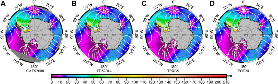
FIGURE 2. Cotidal chart of the M2 constituent of (A) CATS2008, (B) FES2014, (C) TPXO9, and (D) EOT20. Gray values in (A) are locations beyond the geographic coverage of CATS2008. The color scale represents the amplitude value; white contour lines represent the phase lag (°).

FIGURE 3

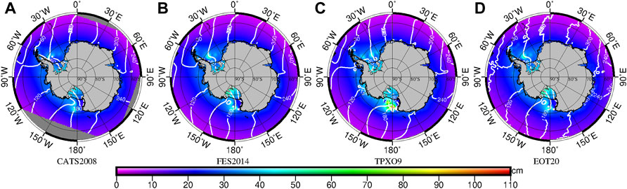
FIGURE 3. Cotidal chart of the K1 constituent of (A) CATS2008, (B) FES2014, (C) TPXO9, and (D) EOT20. Gray values in (A) are locations beyond the geographic coverage of CATS2008. The color scale represents the amplitude value; white contour lines represent the phase lag (°).

Figure 4 and Figure 5 show the differences of M2 and K1 amplitudes and phases between the CATS2008 and FES 2014, TPXO9, and EOT20 models. It can be seen from Figure 4 and Figure 5 that the amplitude differences of models in the open ocean are less than 5 cm, which indicates that there is a strong consistency of the models in the deep ocean. The main differences between the models appear in the areas around the continent. The areas with a large difference in the M2 tidal amplitude are mainly in the Weddell Sea, FRIS, and AIS. The amplitude difference between CATS2008 and FES2014 and EOT20 in the FRIS is more than 20 cm, and the amplitude difference between CATS2008 and TPXO9 in the Weddell Sea and FRIS is more than 20 cm. The phase differences of the M2 are mainly in the Weddell Sea, RIS, and open ocean of the Ross Sea. The phase differences between CATS2008 and FES2014 and EOT20 are small in the Weddell Sea but large in the RIS and open area of Ross Sea. The differences between CATS2008 and TPXO9 in the three regions are large. These three regions are semidiurnal tide amphidromic point areas, and the amplitude changes rapidly.

FIGURE 4

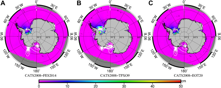
FIGURE 4. Difference of the M2 constituent between (A) CATS2008 and FES2014, (B) CATS2008 and TPXO9, and (C) CATS2008 and EOT20. The color scale represents the amplitude value; white contour lines represent the phase lag (°).

FIGURE 5

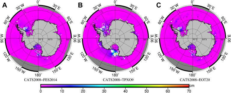
FIGURE 5. Difference of the K1 constituent between (A) CATS2008 and FES2014, (B) CATS2008 and TPXO9, and (C) CATS2008 and EOT20. The color scale represents the amplitude value; white contour lines represent the phase lag (°).

The differences of K1 amplitude are large mainly in the Weddell Sea, Antarctic Peninsula, RIS, and open ocean. The amplitude difference between CATS2008 and FES2014 and EOT20 is more than 20 cm in the Weddell Sea and RIS, the amplitude difference between CATS2008 and TPXO9 is more than 20 cm in the Weddell Sea and open ocean of the Ross Sea, and even more than 60 cm in some areas. The phase differences of K1 are larger mainly in the Weddell Sea and open ocean of the Ross Sea. The differences between CATS2008 and FES2014 are less than those between CATS2008 and TPXO9 in these two regions. The main reasons for the large differences of amplitude and phase in these areas are the enhancement of the influence of seabed topography, seabed friction coefficient, and other parameters, such as the acceleration of the spatial variation of tides, seasonal variation of sea ice, rapid decline of the accuracy of satellite altimetry data in these areas, and some areas beyond the coverage of T/P and other high-precision satellite altimeter missions, all of which lead to the large amplitude difference between models.

4.2 Evaluation of Tide Models in the Antarctic Ocean Using Tidal Records

Bilinear interpolation was used to interpolate the harmonic constants of eight main tidal components, M2, S2, N2, K2, K1, O1, P1, and Q1 to the position of tide gage stations. Eqs 1, 2 were used to calculate the RMS and RSS, and the results are shown in Table 2.

TABLE 2

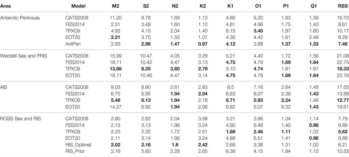
TABLE 2. Comparison between five tide models and tidal records for eight main constituents in the Antarctic Peninsula, Weddell Sea and FRIS, AIS, and Ross Sea and RIS. Bold values denote the smallest RMS and RSS values. (Unit: cm).

4.2.1 Antarctic Peninsula

The Antarctic Peninsula is located at the northernmost end of the Antarctic continent, bordering the Weddell Sea and the Bellinsgauzen Sea in the East and West. The continental shelf in the northwest of the Peninsula extends eastward to the South Shetland Islands. The continental shelf in the southeast of the Peninsula is wider than that in the northwest, and there is Filchner continental ice in the East. There are also many tide gage records in the Antarctic Peninsula, most of which are observed using a pressure tide gauge.

Statistics of RMS and RSS of five models (including CATS 2008, FES 2014, TPXO9, EOT20, and AntPen) in the Antarctic Peninsula are recorded in Table 2. The RMS of N2, K2, P1, and Q1 is small and almost the same. The minimum RMS of M2 is EOT20, and the minimum RMS of K1 is TPXO9. RMS of FES2014 and EOT20 is very similar. South of 66°S, the value of FES2014 is adopted in the EOT20. From the RSS values, the models with the same precision in the Antarctic Peninsula are FES 2014, EOT20, and AntPen models, which are 8.61, 8.29, and 7.46 cm, respectively; CATS2008 and TPXO9 models are in the order of magnitude of 10 cm. The accuracy of FES 2014, EOT20, and AntPen is higher than that of the other two tide models in the Antarctic Peninsula.

As can be seen from Figure 6, the RSS values calculated by each model on the west side of the Antarctic Peninsula are less than 3 cm. In the eastern side of the Antarctic Peninsula, in the Larsen Ice Shelf, the RSS calculated by each model is large, about 5–10 cm. Compared with the global model FES 2014 (Figure 6B), TPXO9 (Figure 6C), EOT20 (Figure 6D), and regional tide model AntPen (Figure 6E), the RSS values of CATS 2008 (Figure 6A) of four stations on the South Shetland Island are larger, and the RSS values of TPXO9 of five stations on Larsen C Ice Shelf are larger.

FIGURE 6

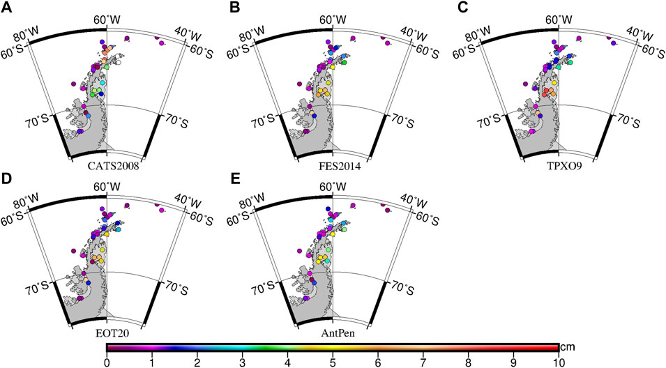
FIGURE 6. RSS of each station in the Antarctic Peninsula of (A) CATS2008, (B) FES2014, (C) TPXO9, (D) EOT20, and (E) AntPen.

4.2.2 The Weddell Sea and FRIS

The Weddell Sea is one of the epeiric seas in Antarctica, and there is FRIS in the south. There are many kinds of tide gage stations in the Weddell Sea and FRIS, and the observation data are the most, so the best basis for the verification of the model can be provided.

The RMS and RSS values of four models (including CATS 2008, FES 2014, TPXO9, and EOT20) in the Weddell Sea and FRIS are also shown in Table 2. The RMS of semidiurnal tide is higher than the ones of the diurnal tide, which is consistent with the distribution of tidal amplitude. It can be seen from Figure 2 and Figure 3 that the amplitude of M2 is larger in the FRIS and that of K1 is smaller in FRIS. Among the four models, TPXO9 has the smallest RSS value, followed by CATS 2008, FES 2014, and EOT20. TPXO9 is the most accurate model for the Weddell Sea and FRIS region.

It can be seen from Figure 7 that the RSS values calculated by GPS stations and gravity stations far away from the FRIS in the Weddell Sea area are relatively small, while the RSS values calculated by stations on the FRIS are relatively large. The areas of large RSS are mainly concentrated in the west of the ice shelf, which contains Evans and other ice streams. The accuracy of FES 2014 (Figure 7B) and EOT20 (Figure 7D) models is worse than those of CATS 2008 (Figure 7A) and TPXO9 (Figure 7C) models. The interaction between the ice stream and ice shelf has an impact on the ocean tide and altimetry data, which leads to poor prediction accuracy of the model.

FIGURE 7

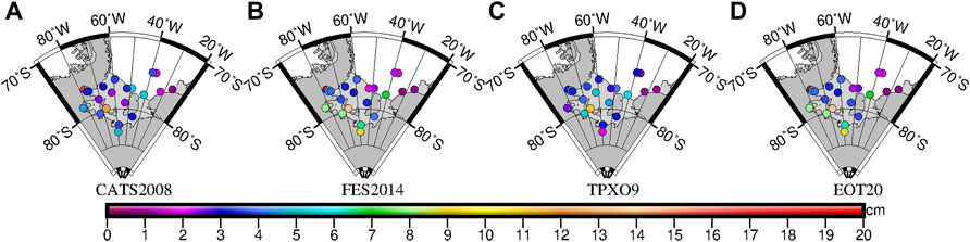
FIGURE 7. RSS of each station in the Weddell Sea and FRIS of (A) CATS2008, (B) FES2014, (C) TPXO9, and (D) EOT20.

4.2.3 Amery Ice Shelf

The number of observation stations on the AIS is less, and the observation time of observation stations on the AIS is relatively short.

Table 2 also makes statistics on RMS and RSS of four models (including CATS 2008, FES 2014, TPXO9, and EOT20) in the AIS. The accuracy of RMS of CATS2008 for each tide constituent is the worst, and the accuracy of RMS of TPXO9 for each tide constituent is the best. The accuracy of TPXO9 in the AIS is the highest, and RSS is 12.77 cm, which may be the result of the assimilation of some tide gage stations in this area by TPXO9. The accuracy of the CATS2008 is the worst, at 17.55 cm.

It can be seen from Figure 8 that the accuracies of CATS 2008 (Figure 8A), FES 2014 (Figure 8B), and TPXO9 (Figure 8C) at each station (except the one at the highest latitude) are almost the same, about 0–4 cm, and the station with the worst accuracy is the station at the highest latitude. Although the EOT20 (Figure 8D) adopted the results of FES2014 in the south of 66°S, the accuracy of EOT20 was different from that of FES2014 due to its lower resolution.

FIGURE 8

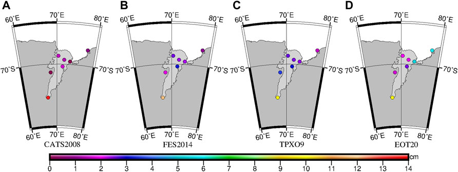
FIGURE 8. RSS of each station in the AIS of (A) CATS2008, (B) FES2014, (C) TPXO9, and (D) EOT20.

4.2.4 The Ross Sea and RIS

The Ross Sea is the bay of the South Pacific deep into Antarctica, and the RIS is the largest one in the world. Since the tide gage data of the RIS are the data records for more than 29 days, it is of great significance for tide analysis and model comparison.

The RMS and RSS of six models in the Ross Sea and RIS, including CATS2008, FES2014, TPXO9, EOT20, Ross_Prior (Model_Ross_Prior), and Ross_Optimal (Model_Ross_Tim) can be seen in Table 2. The RMS of K1 and O1 is larger than that of M2 and S2, which is consistent with the distribution of tide constituent amplitude in Figure 2 and Figure 3. For K1, O1, and Q1, the accuracy of RMS of TPXO9 is the best, and the accuracy of RMS of RIS_Prior is the worst. For M2 and S2, the accuracy of RMS of each model is almost the same. It can be seen from RMS that the accuracy of the eight tide constituents of TPXO9 and Ross_Optimal model is high. The accuracy of RMS and RSS of Ross_Prior is significantly lower than that of the other five models, mainly due to the Ross_Prior model being a hydrodynamic model, no data are assimilated. In this region, TPXO9 and Ross_Optimal models have the highest accuracy, and the RSS values are 5.62 and 6.21 cm.

As can be seen from Figure 9, RSS in the Ross Sea increases with the increase of latitude. On the western side of the RIS, the accuracies of TPXO9 (Figure 9C) and ROSS_Optimal (Figure 9E) are significantly higher than those of other models, and the accuracies of FES 2014 (Figure 9B), EOT20 (Figure 9D), and ROSS_Prior (Figure 9F) are lower. On the eastern side of the Ross Sea and RIS, the accuracy of CATS 2008 (Figure 9A) is significantly high, and the accuracy of ROSS_Prior (Figure 9F) is the lowest.

FIGURE 9

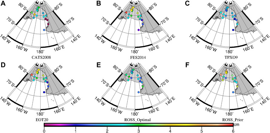
FIGURE 9. RSS of each station of (A) CATS2008, (B) FES2014, (C) TPXO9, (D) EOT20, (E) ROSS_Optimal, and (F) ROSS_Prior in the Ross Sea and RIS.

4.3 Evaluation of Tide Models in the Antarctic Ocean Using Satellite Altimetry Along-Track Harmonic Constants

Satellite altimetry data are an important supplement for the validation of tide models. Although the satellite altimeter is affected by the satellite orbital error and space propagation error, a large amount of data can be obtained along the orbit. Eqs 1, 2 were used to calculate RMS and RSS in the Drake Passage, Kerguelen Islands, and Adelie–Mertz, and the results are statistically studied and shown in Table 3.

TABLE 3

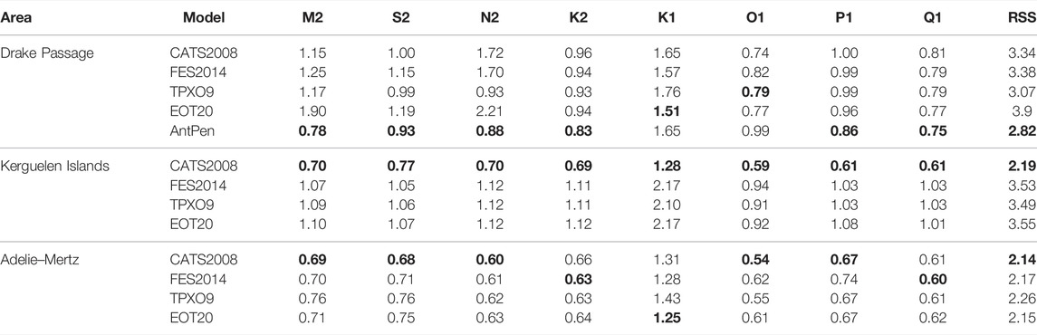
TABLE 3. Comparison between five tide models and tidal records for eight main constituents in the Drake Passage, Kerguelen Islands, and Adelie–Mertz. Bold values denote the smallest RMS and RSS values. (Unit: cm).

4.3.1 Drake Passage

The RMS and RSS values of five models (including CATS 2008, FES 2014, TPXO9, EOT20, and AntPen) and satellite altimeter along-track harmonic constants in the Drake area are statistically analyzed in Table 3. The RMS of O1, P1, Q1, and S2 is small. The RMS of K1 simulated by each model is larger than that of other tide constituents. From the RSS values, the model with the highest accuracy in the Drake Passage is AntPen, followed by TPXO9, which are 2.82 and 3.07 cm. One of the possible reasons for the better results of the AntPen model is that it does not completely cover the coordinates of satellite points in the region.

As can be seen from Figure 10, at the 50°W∼70°W and 55°S∼60°S region, the RSS calculated by each model is larger, ranging from 1 to 4 cm. This region is located in the Antarctic circulation region, and the errors caused by ocean dynamic phenomena are not well-corrected in satellite altimeter data, which has led to a large error in the calculation of harmonic constants. The RSS values of other areas are smaller, ranging from 0 to 2 cm. In addition, it can be seen from Figure 10 that the RSS of satellite points at the original orbit is less than that of the interleaved orbit, and the RSS values of satellite points at the original orbit are less than 2 cm, which are less than those of the interleaved orbit, which is about 2–4 cm. The regions with larger RSS values are distributed at the locations of the Antarctic Circumpolar Current (ACC) fronts (Donohue et al., 2016). Meandering ACC fronts created elevated Sea Surface Height Anomaly (SSHA) variance in the northern Drake Passage; therefore, the harmonic constants calculated based on SSHA have larger errors.

FIGURE 10

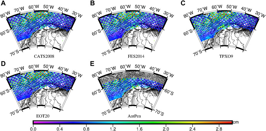
FIGURE 10. RSS of each along-track point of (A) CATS2008, (B) FES2014, (C) TPXO9, (D) EOT20, and (E) AntPen in the Drake Passage, including original orbit (large points) and interleaved orbit (small points). Gray values in (E) are locations beyond the geographic coverage of the AntPen model.

4.3.2 Kerguelen Islands

The RMS and RSS values of four models (including CATS 2008, FES 2014, TPXO9, and EOT20) and satellite altimetry along-track harmonic constants are also statistically analyzed in Table 3. The RMS of each tide constituent of CATS2008 is less than that of TPXO9 and FES 2014. From the RSS values, the model with the highest accuracy in the Kerguelen Islands is CATS2008, which is 2.19 cm. The RMS of K1 of each model is larger than that of other tide constituents. It is located near the amphidromic point of the AIS. As can be seen from Figure 11, the RSS values of satellite points at the original orbit are less than 1.5 cm, which is smaller than those of the interleaved orbit, about 1–3 cm. The RSS values are relatively larger between 80°–90°E and 55°–60°S. The SSHA data are affected by the Southern ACC Front in this region (Park et al., 2008; Wang et al., 2016).

FIGURE 11

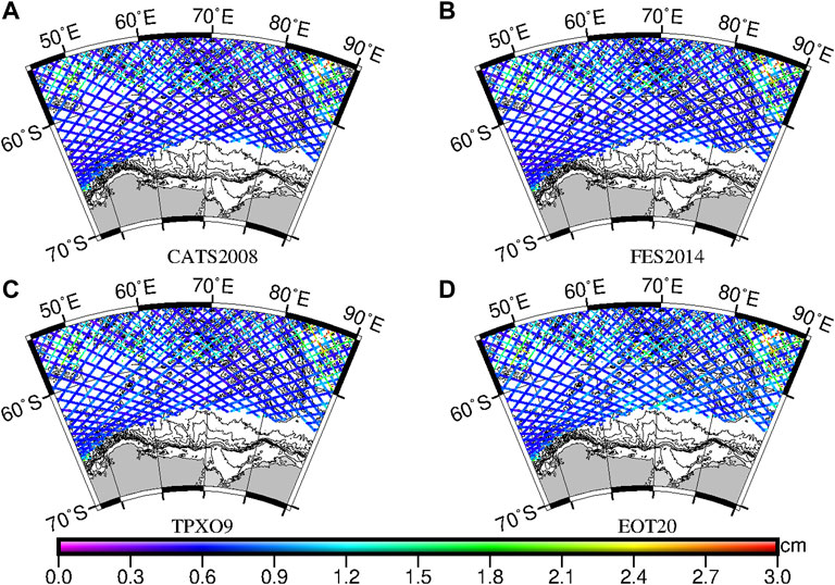
FIGURE 11. RSS of each along-track point of (A) CATS2008, (B) FES2014, (C) TPXO9, and (D) EOT20 in the Kerguelen Islands, including original orbit (large points) and interleaved orbit (small points).

4.3.3 Adelie–Mertz

Table 3 also shows RMS and RSS of four models (including CATS2008, FES2014, TPXO9, and EOT20) and satellite altimeter along-track harmonic constituents in the Adelie–Mertz. There is no significant difference in the indicators of the eight tide constituents. The RMS of K1 of each model is large. From the RSS values, the model with the highest accuracy in the Adelie–Mertz is CATS 2008, followed by EOT20, FES 2014, and TPXO9, which are 2.14, 2.15, 2.17, and 3.07 cm, respectively. The results of the four models are similar. As can be seen from Figure 12, the RSS values of the satellite point at the original orbit are less than 1.5 cm, which are smaller than those of the satellite point at the interleaved orbit, about 1–2 cm.

FIGURE 12

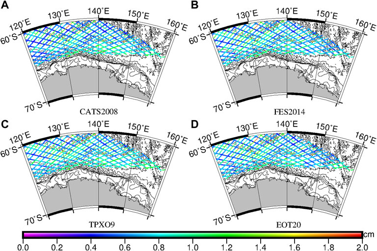
FIGURE 12. RSS of each along-track point of (A) CATS2008, (B) FES2014, (C) TPXO9, and (D) EOT20 in the Adelie-Mertz, including original orbit (large points) and interleaved orbit (small points).

4.4 Standard Deviation in Satellite Altimetry Observations

The L2P products distributed from Archiving, Validation, and Interpretation of Satellite Oceanographic Data (AVISO) contain time, sea level anomaly (SLA), information of validity of the data, and all corrections which are necessary to compute the SLA. We use non-time critical altimeter SLA products computed with respect to a 20-year (1993-2012) mean profile for Sentinel-3A. The time period of Sentinel-3A spans from March 2016 to December 2021 (from cycle1 to cycle 80). Sentinel-3A is fully independent of all the tide models tested, and Sentinel-3A is used with a new generation synthetic aperture radar altimetry, which enables more accurate SSH data closer to the coast compared with traditional altimeters. Cycle 54 was selected to estimate ocean tide models.

To compare the four ocean tide models, the four tide models were used to predict the tidal height at the single satellite crossovers between ascending and descending tracks around Antarctica and then the tidal height was applied to correct the SLA at single-satellite crossovers, and thus the SLA residuals after tidal corrections from the three tide models can be obtained. The standard deviation (STD) of the crossover points is calculated, as shown in Table 4.

TABLE 4

TABLE 4. STD of the SSH residuals at dual satellite crossovers before and after tidal correction. Bold values denote the smallest STD value (Unit: cm).

Table 4 lists the comparison between the four tide models at single-satellite crossovers. After the tidal correction of each model, the STD of crossover points has been greatly improved. The results demonstrate a good performance of the FES2014 tidal solution compared to the other two models, the STD is reduced from 36.17 to 14.75 cm.

5 Discussion

M2 and K1 tidal charts of the latest global tide models FES 2014, TPXO9, EOT20, and the latest Antarctic tide model CATS2008 are compared around Antarctica (Figure 2 and Figure 3). The amplitude of each tide model in the open ocean is the same, and there is a big difference between the coastal area and the ice shelf area, up to 70 cm. The phase distributions of each model are consistent in the open ocean, and the differences in the offshore area are mainly reflected in the location of the amphidromic point. The locations of the amphidromic point of M2 are quite different in the Weddell Sea, RIS, and open ocean of Ross Sea. There is no amphidromic point of K1 in the Antarctic Ocean, and the accuracy of the K1 phase of the four models is good.

The accuracies of the models in the Antarctic Peninsula, Weddell Sea and FRIS, AIS, and Ross Sea and RIS were analyzed using the tide records in coastal and ice shelf regions. The results show that AntPen has the highest accuracy in the Antarctic Peninsula region, while TPXO9 is the most accurate model in other regions, consistent with its assimilation of many situ data records. The accuracy of models is poorer in the Weddell Sea and FRIS than that in other regions. First, the latitude of the Weddell Sea is higher, and the satellite altimeter data assimilated is less, so the accuracy is poor. Second, most of the observation data used for accuracy evaluation comes from GPS observation, gravity observation, and visual tide staff, and these data are intermediate-length records and have lower accuracy.

From the analysis of the three regions of Drake Passage, Kerguelen Islands, and Adelie–Mertz from X-TRACK, it can be concluded that the errors of the interleaved orbit are less than those of the original orbit because they are located in the open ocean, the accuracy of each model is almost the same. The distribution of RSS in the deep ocean is consistent with the Antarctic Circulation Current fronts, and RSS is larger in the region where the fronts are located. The amplitude error of K1 is larger than other constituents, which is about two times that of other tide constituents. We infer that because the alias synodic periods (about 9.317 years) of K1/Ssa constituents are relatively longer than other pair constituents (Andersen and Knudsen, 1997), it caused the poor accuracy of K1 extracted from satellite altimetry data.

The STDs of crossover difference from the Sentinel-3A showed significant reduction after the ocean tide model correction. The STD is smallest after being corrected by FES2014. There are still differences at the crossover due to the combined effect of tidal residuals, unsimulated surface circulation, and high-frequency atmospheric effects (Seifi et al., 2019).

Limitations are found in using RMS and RSS to evaluate ocean tide models. First, there is no comparison between the short-period tides and long-period tides, and only eight major tidal constituents are compared. The comparison is incomplete. Second, due to the different resolutions of each model, errors will be generated when extracting harmonic constants at each point using interpolation methods.

6 Conclusion

This study summarized the research work of the global tide models widely applied in the Antarctic area, the construction of the tide models around the Antarctic area, and the construction of the tide models of the typical Antarctic area. The mutual differences were compared, and the accuracy of the tide models is evaluated using the data of tide gage and satellite altimeter. The RSS of inshore and ice shelf tide gages is larger than that of satellite altimeter. The model accuracy at the inshore tide gauge station varies from region to region, about 5–23 cm, and the model accuracy at the satellite altimeter point in the open and deep ocean is less than 4 cm. The precision of TPXO9 is relatively high in inshore areas and ice shelf areas, and the accuracy of the tidal model is relatively consistent in deep oceans.

At present, there are big differences between the accuracy of tide models in the polar region and open ocean area. To narrow the differences, efforts should be taken in the following aspects: 1) The location accuracy of the grounding line should be improved in the coastal areas and ice shelf areas. 2) The latest water depth model is used to improve the water depth data, especially the water depth under the large ice shelf. Currently, the water depth models widely used include GEBCO, ETOPO1, and IBCSO in the Antarctic region. 3) High-quality altimetry data are added for model construction. On the one hand, the mechanism of sea ice changes should be further studied to weaken the seasonal influence of sea ice on altimetry data; on the other hand, the data of ICESat-2, HY-2A, Sentinel-3, and other satellites should be integrated to effectively improve the spatial and temporal resolution of satellite altimetry data. Wide swath altimetry SWOT will fly over some polar regions; the high spatial resolution of altimetry will help solve the problem of short-scale tides. 4) More tide gages should be built so that high-quality measured tide data will be added for model construction and validation. For example, it is suggested to install the bottom pressure tide gages near the Weddell Sea, where there are semidiurnal tide amphidromic points and the tide changes are complex.

Data Availability Statement

The original contributions presented in the study are included in the article/Supplementary Material, further inquiries can be directed to the corresponding author.

Author Contributions

Conceptualization, XZ and WS; methodology, WS and DZ; data curation, XZ, WS, and FS; writing—original draft preparation, WS; writing—review and editing, WS and FS; visualization, WS and FS; supervision, XZ; project administration, DZ; funding acquisition, DZ All the authors have read and agreed to the published version of the manuscript.

Funding

This research was funded by the National Natural Science Foundation of China (Grant Numbers 41706115 and 42104035) and the Natural Science Foundation of Shandong Province (Grant Numbers ZR2020QD087 and ZR2017QD011).

Conflict of Interest

Author YS was employed by the Qingdao West Coast Basic Geographic Information Center Co. Ltd.

The remaining authors declare that the research was conducted in the absence of any commercial or financial relationships that could be construed as a potential conflict of interest.

Publisher’s Note

All claims expressed in this article are solely those of the authors and do not necessarily represent those of their affiliated organizations, or those of the publisher, the editors, and the reviewers. Any product that may be evaluated in this article, or claim that may be made by its manufacturer, is not guaranteed or endorsed by the publisher.

Acknowledgments

The author would like to thank Earth and Space Research for providing harmonic constants (https://www.esr.org/data-products/antarctic_tg_database/atg-data/) (http://www.esr.org/tic_tg_index.html). We are grateful to the Center for Topographic studies of the Oceans and Hydrosphere (CTOH) for the processing of the altimeter observations and the generation of the X-TRACK product used for this study. We thank AVISO for providing the Sentinel-3A L2P data (ftp://ftp-access.aviso.altimetry.fr). CATS2008 and other regional models can be downloaded via https://www.esr.org/research/polar-tide-models/list-of-polar-tide-models/. FES2014 is available online (https://www.aviso.altimetry.fr/es/data/products/auxiliary-products/global-tide-fes/description-fes2014.html). TPXO9 is available online https://www.tpxo.net/global. EOT20 is available online https://www.seanoe.org/data/00683/79489/.

References

Andersen, O. B., and Knudsen, P. (1997). Multi-satellite Ocean Tide Modelling—The K1 Constituent. Prog. Oceanogr. 40 (1-4), 197–216. doi:10.1016/S0079-6611(98)00002-0

CrossRef Full Text | Google Scholar

Carrère, L., Lyard, F., Cancet, M., and Guillot, A. (2016). “FES 2014, a New Tidal Model—Validation Results and Perspectives for Improvements,” in Proceedings of the ESA Living Planet Symposium. Editor L. Ouwehand (Prague, Czech Republic: European Space Agency. 9–13 May 2016.

Google Scholar

Carrère, L., Lyard, M., Cancet, M., Guillot, A., Roblou, L., and Guillot, A. (2012). “FES2012: A New Global Tidal Model Taking Advantage of Nearly 20 Years of Altimetry,” in Proceedings of the 20 Years of Progress in Radar Altimetry Symposium. Editor L. Ouwehand (Venice, Italy: European Space Agency. 24–29 September 2012.

Google Scholar

Cheng, Y., and Andersen, O. B. (2011). Multimission Empirical Ocean Tide Modeling for Shallow Waters and Polar Seas. J. Geophys. Res. 116, C11001. doi:10.1029/2011JC007172

CrossRef Full Text | Google Scholar

Donohue, K. A., Kennelly, M. A., and Cutting, A. (2016). Sea Surface Height Variability in Drake Passage. J. Atmos. Ocean. Technol. 33 (4), 669–683. doi:10.1175/jtech-d-15-0249.1

CrossRef Full Text | Google Scholar

Egbert, G. D., and Erofeeva, S. Y. (2002). Efficient Inverse Modeling of Barotropic Ocean Tides. J. Atmos. Oceanic Technol. 19, 183–204. doi:10.1175/1520-0426(2002)019<0183:eimobo>2.0.co;2

CrossRef Full Text | Google Scholar

Egbert, G. D., and Ray, R. D. (2000). Significant Dissipation of Tidal Energy in the Deep Ocean Inferred from Satellite Altimeter Data. Nature 405, 775–778. doi:10.1038/35015531

PubMed Abstract | CrossRef Full Text | Google Scholar

Egbert, Y., Gary, D., and Erofeeva, S. (2018). “TPXO9, A New Global Tidal Model in TPXO Series,” in Proceedings of the Ocean Science Meeting (Portland, OR, USA: American Geophysical Union. 11–16 February 2018.

Google Scholar

Erofeeva, S. Y., Padman, L., and Egbert, G. (2005). Assimilation of Ship-Mounted ADCP Data for Barotropic Tides: Application to the Ross Sea. J. Atmos. Ocean. Technol. 22, 721–734. doi:10.1175/JTECH1735.1

CrossRef Full Text | Google Scholar

Fok, H. S. (2012). “Ocean Tides Modeling Using Satellite Altimetry,” in Geodetic Science Rep (Columbus: Ohio State Univ.), 501.

Google Scholar

Hart-Davis, M. G., Piccioni, G., Dettmering, D., Schwatke, C., Passaro, M., and Seitz, F. (2021). EOT20: A Global Ocean Tide Model from Multi-mission Satellite Altimetry. Earth Syst. Sci. Data Discuss. 13, 3869–3884. doi:10.5194/essd-13-3869-2021

CrossRef Full Text | Google Scholar

Hemer, M. A., Hunter, J. R., and Coleman, R. (2006). Barotropic Tides beneath the Amery Ice Shelf. J. Geophys. Res. 111 (C11), C11008. doi:10.1029/2006JC003622

CrossRef Full Text | Google Scholar

Kim, T.-H., Shibuya, K., Doi, K., Aoyama, Y., and Hayakawa, H. (2011). Validation of Global Ocean Tide Models Using the Superconducting Gravimeter Data at Syowa Station, Antarctica, and In Situ Tide Gauge and Bottom-Pressure Observations. Polar Sci. 5, 21–39. doi:10.1016/j.polar.2010.11.001

CrossRef Full Text | Google Scholar

King, M. A., and Padman, L. (2005). Accuracy Assessment of Ocean Tide Models Around Antarctica. Geophys. Res. Lett. 32, L23608. doi:10.1029/2005GL023901

CrossRef Full Text | Google Scholar

King, M. A., Penna, N. T., Clarke, P. J., and King, E. D. (2005). Validation of Ocean Tide Models Around Antarctica Using Onshore GPS and Gravity Data. J. Geophys. Res. 110 (B8), B08401. doi:10.1029/2004JB003390

CrossRef Full Text | Google Scholar

Lefèvre, F., Lyard, F. H., Le Provost, C., and Schrama, E. J. O. (2002). FES99: A Global Tide Finite Element Solution Assimilating Tide Gauge and Altimetric Information. J. Atmos. Oceanic Technol. 19, 1345–1356. doi:10.1175/1520-0426(2002)019<1345:fagtfe>2.0.co;2

CrossRef Full Text | Google Scholar

Lei, J., Li, F., Zhang, S., Ke, H., Zhang, Q., and Li, W. (20172017). “Accuracy Assessment of Recent Global Ocean Tide Models Around Antarctica,” in Int. Arch. Photogramm. Remote Sens. Spatial Inf. Sci. Editor D. Li (Wuhan, China: International Society of Photogrammetry and Remote Sensing, XLII-2/W7, 1521–1528. doi:10.5194/isprs-archives-xlii-2-w7-1521-2017

CrossRef Full Text | Google Scholar

Lyard, F. H., Allain, D. J., Cancet, M., Carrère, L., and Picot, N. (2020). FES2014 Global Ocean Tide Atlas: Design and Performance. Ocean Sci. 17, 615–649. doi:10.5194/os-17-615-2021

CrossRef Full Text | Google Scholar

Lyard, F., Lefevre, F., Letellier, T., and Francis, O. (2006). Modelling the Global Ocean Tides: Modern Insights from FES2004. Ocean Dyn. 56, 394–415. doi:10.1007/s10236-006-0086-x

CrossRef Full Text | Google Scholar

Matsumoto, K., Takanezawa, T., and Ooe, M. (2000). Ocean Tide Models Developed by Assimilating TOPEX/POSEIDON Altimeter Data into Hydrodynamical Model: A Global Model and a Regional Model Around Japan. J. Oceanogr. 56, 567–581. doi:10.1023/A:1011157212596

CrossRef Full Text | Google Scholar

Oreiro, F. A., D'Onofrio, E., Grismeyer, W., Fiore, M., and Saraceno, M. (2014). Comparison of Tide Model Outputs for the Northern Region of the Antarctic Peninsula Using Satellite Altimeters and Tide Gauge Data. Polar Sci. 8, 10–23. doi:10.1016/j.polar.2013.12.001

CrossRef Full Text | Google Scholar

Padman, L., Erofeeva, S., and Joughin, I. (2003). Tides of the Ross Sea and Ross Ice Shelf Cavity. Antartic Sci. 15 (1), 31–40. doi:10.1017/S0954102003001032

CrossRef Full Text | Google Scholar

Padman, L., and Erofeeva, S. (2005). Tide Model Driver (TMD) Manual; Earth & Space Research: Seattle WA, USA. Available at: https://svn.oss.deltares.nl/repos/openearthtools/trunk/matlab/applications/DelftDashBoard/utils/tmd/Documentation/README_TMD_vs1.2.pdf, November 28, 2005.

Google Scholar

Padman, L., Erofeeva, S. Y., and Fricker, H. A. (2008). Improving Antarctic Tide Models by Assimilation of ICESat Laser Altimetry over Ice Shelves. Geophys. Res. Lett. 35, L22504. doi:10.1029/2008GL035592

CrossRef Full Text | Google Scholar

Padman, L., Fricker, H. A., Coleman, R., Howard, S., and Erofeeva, L. (2002). A New Tide Model for the Antarctic Ice Shelves and Seas. Ann. Glaciol. 34, 247–254. doi:10.3189/172756402781817752

CrossRef Full Text | Google Scholar

Padman, L., and Fricker, H. A. (2005). Tides on the Ross Ice Shelf Observed with ICESat. Geophys. Res. Lett. 32, 1–7. doi:10.1029/2005GL023214

CrossRef Full Text | Google Scholar

Padman, L., and Kottmeier, C. (2000). High-frequency Ice Motion and Divergence in the Weddell Sea. J. Geophys. Res. 105 (C2), 3379–3400. doi:10.1029/1999JC900267

CrossRef Full Text | Google Scholar

Park, Y.-H., Roquet, F., Durand, I., and Fuda, J.-L. (2008). Large-scale Circulation over and Around the Northern Kerguelen Plateau. Deep Sea Res. Part Topical Stud. Oceanography 55, 566–581. doi:10.1016/j.dsr2.2007.12.030

CrossRef Full Text | Google Scholar

Ray, R. D. (1999). “A Global Ocean Tide Model from TOPEX/Poseidon Altimetry: GOT99.2,” in NASA Tech. Memo. 209478 (Greenbelt, MD: Goddard Space Flight Center), 58.

Google Scholar

Ray, R. D. (2013). Precise Comparisons of Bottom-Pressure and Altimetric Ocean Tides. J. Geophys. Res. Oceans 118, 4570–4584. doi:10.1002/jgrc.20336

CrossRef Full Text | Google Scholar

Robertson, R., Padman, L., and Egbert, G. D. (1998). “Tides in the Weddell Sea,” in proceedings of Ocean, Ice, and Atmosphere, Interactions at the Antarctic Continental Margin. Antarctic Research Series. Editors S. S. Jacobs, and R. F. Weiss (Washington, DC: American Geophysical Union), 341–369. doi:10.1029/AR075p034175

CrossRef Full Text | Google Scholar

Roblou, L., Lamouroux, J., Bouffard, J., Lyard, F., Le Hénaff, M., Lombard, A., et al. (2011). “Post-processing Altimeter Data towards Coastal Applications and Integration into Coastal Models,” in Coastal Altimetry. Editors S. Vignudelli, A. G. Kostianoy, P. Cipollini, and J. Benveniste (Berlin/Heidelberg, Germany: Springer), 217–246. doi:10.1007/978-3-642-12796-0_9

CrossRef Full Text | Google Scholar

Savcenko, R., and Bosch, W. (2012). EOT11a—Empirical Ocean Tide Model from Multi-mission Satellite Altimetry. München, Germany: Deutsches Geodätisches Forschungsinstitut. DGFI Report No. 89.

Google Scholar

Seifi, F., Deng, X., and Baltazar Andersen, O. (2019). Assessment of the Accuracy of Recent Empirical and Assimilated Tidal Models for the Great Barrier Reef, Australia, Using Satellite and Coastal Data. Remote Sensing 11 (10), 1211. doi:10.3390/rs11101211

CrossRef Full Text | Google Scholar

Smithson, M. J., Robinson, A. V., and Flather, R. A. (1996). Ocean Tides under the Filchner-Ronne Ice Shelf, Antarctica. Ann. Glaciol. 23, 217–225. doi:10.3189/S0260305500013471

CrossRef Full Text | Google Scholar

Stammer, D., Ray, R. D., Andersen, O. B., Arbic, B. K., Bosch, W., Carrère, L., et al. (2014). Accuracy Assessment of Global Barotropic Ocean Tide Models. Rev. Geophys. 52, 243–282. doi:10.1002/2014RG000450

CrossRef Full Text | Google Scholar

Taguchi, E., Stammer, D., and Zahel, W. (2014). Inferring Deep Ocean Tidal Energy Dissipation from the Global High-Resolution Data-Assimilative HAMTIDE Model. J. Geophys. Res. Oceans 119, 4573–4592. doi:10.1002/2013JC009766

CrossRef Full Text | Google Scholar

Wang, J., Mazloff, M. R., and Gille, S. T. (2016). The Effect of the Kerguelen Plateau on the Ocean Circulation. J. Phys. Oceanogr 46 (11), 3385–3396. doi:10.1175/jpo-d-15-0216.1

CrossRef Full Text | Google Scholar