Source-Free P-SV Converted-Wave Reverse-Time Migration Using First-Order Velocity-Dilatation-Rotation Equations

The cross-correlation imaging condition between source- and receiver-wavefields is often used in the elastic wave reverse-time migration (RTM) to utilize P- and S-waves. However, it cannot be applied in the absence of source information (e.g., source location, and source wavelet), which is quite common in passive source exploration. We employ a source-free P-SV converted-wave imaging condition, which only requires the back-propagating receiver-wavefield to utilize the P-SV converted waves in imaging the subsurface structures. The imaging condition is independent of source information, which can avoid the extrapolation and reconstruction of the source-wavefield. As a result, the computational cost is decreased to about one-third of conventional RTM that uses source-wavefield reconstruction strategies, e.g., random boundaries. The memory requirement could be also reduced by avoiding the calculation of source-wavefield. Because our imaging condition uses the vector P-wavefield and vector S-wavefield to utilize the P-SV waves, it is necessary to decouple P-wavefield and S-wavefield during the reverse-time extrapolation of receiver-wavefield. We use the first-order velocity-dilatation-rotation elastic wave equations to realize the reverse-time propagation of vector receiver-wavefield, where the vector P-wavefield and vector S-wavefield can be obtained directly. Based on the above methods, a source-free P-SV converted-wave RTM of multi-component seismic data is realized. The model tests show that this method can generate promising subsurface images and can be complementarily used when conventional cross-correlation imaging conditions are not suitable.

Introduction

Techniques based on reflected P-wave have played an important role in seismic exploration. However, with the continued improvement of seismic exploration accuracy and the increased complexity of exploration targeted structure and lithology in the oil and gas industry, seismic exploration based solely on reflected P-wave is progressively restricted by its theoretical assumptions and single wavefield information. It has become challenging to obtain satisfactory imaging results for exploring fractured carbonate, coalbed methane, and shale gas reservoirs (Stewart et al., 2003; Yang et al., 2006; Bian et al., 2017). Multi-component seismic exploration based on the elastic wave theory can obtain more subsurface imaging information. Compared with the reflected P-wave exploration techniques, multi-component seismic imaging methods require fewer theoretical assumptions and take account of S-wave propagation in complex media. In theory, multi-component seismic exploration is more capable of fully characterizing the subsurface using both P- and S-waves, which is more conducive to improving the accuracy and resolution of imaging.

Prestack depth migration is a popular research topic of multi-component seismic exploration. At present, there are two main ways to achieve prestack migration using multi-component seismic data. One is based on scalar wave theory (Whitemore, 1983; Sun and McMechan, 2001; Sun et al., 2006; Chattopadhyay and McMechan, 2008; Liu et al., 2011) to first obtain the reflected P-wave and converted S-wave recordings by decoupling P- and S-waves from multi-component seismic data. Then, the existing acoustic RTM operator is adopted to realize the migration imaging of P- and S-waves data, respectively. It has the advantage of few calculations and high efficiency, but it also has apparent issues in that ignoring the vector properties of elastic waves and the accuracy of P-wave and S-wave decoupling can seriously affect the migration results. The other way is the elastic wave prestack depth migration based on vector wavefield (Chang and McMechan, 1994; He and Zhang, 2006), which is mainly realized by elastic reverse-time migration (ERTM) techniques. It regards multi-component seismic data as a vector wavefield for processing. Generally, the method based on the vector wavefield does not require the decoupling of P- and S-waves in the data domain. By solving the elastic wave equations and combining them with a proper imaging condition, e.g., the joint migration of multi-component, the simultaneous imaging of reflected P-wave and converted S-wave can be obtained. Therefore, the ERTM techniques have attracted extensive attention in the industry.

A large number of studies have been conducted on ERTM in recent years, and significant advancements have been made in wavefield extrapolation (Dellinger and Etgen, 1990; Dong et al., 2000b), imaging methods (He and Zhang, 2006; Du et al., 2012a; Du et al., 2014), decoupling methods of P- and S-waves in the migration process (Sun et al., 2004; Yan and Sava, 2009), migration noise suppression (Yu et al., 2018; Zhang et al., 2021), reverse-time reconstruction of the source-wavefield (Clapp, 2009; Wu and Qin, 2014), and GPU parallelism (Bao et al., 2021; Shen, 2017), respectively. These results are of great significance to promote the development of multi-component seismic RTM techniques. However, the existing ERTM techniques have two main issues. 1) The ERTM techniques assume that each component in the multi-component seismic data has the same seismic frequency spectrum. In fact, due to the different absorption mechanisms of the P-wave and S-wave in the subsurface media (Biot, 1956; Murphy, 1982; Wang et al., 2006), the attenuation of the high-frequency components of the S-wave in the actual recordings is greater than that of the P-wave, resulting in P-wave often having a higher dominant frequency and a broader bandwidth. The spectrum discrepancy of recorded P- and S-waves introduces difficulty in setting the wavelet in ERTM. 2) It is challenging to obtain accurate propagation directions of P- and S-waves for wavefield separation. In the ERTM, cross-correlation imaging condition (Claerbout, 1971) based on wavefield separation is often used to utilize the P- and S-waves, and further suppress low-wavenumber imaging artifacts. The prerequisite for accurate wavefield separation is that the propagation directions of pure P-wavefield and pure S-wavefield at all imaging grid points must be obtained for each timestep. Based on the Poynting vector (Poynting, 1884), the conventional methods for calculating wavefield propagation directions can only get the propagation directions of the coupled wavefield (Du et al., 2012b), rather than that of pure P-wavefield and pure S-wavefield. The error in propagation direction will be transferred to the migration results, reducing the accuracy of the migration.

This paper demonstrates a converted-wave RTM method that can avoid the two issues of existing traditional elastic techniques. The first-order velocity-dilatation-rotation elastic wave equations in the isotropic medium are used to implement the reverse-time extrapolation of the receiver-wavefield. The P-wavefield and S-wavefield can be automatically decoupled during the propagation which we refer to as “wavefield decomposition”. Then the decoupled receiver-wavefields are separated into the pure P- and S-wavefields of different propagation directions based on the Poynting vector which we refer to as “wavefield separation”. This study utilizes the up-going pure P- and S-waves derived from the Poynting vector to realize the converted-wave RTM by using the source-free P-SV converted-wave imaging condition.

The advantages of the method proposed in this study are 1) The first-order velocity-dilatation-rotation elastic wave equations explicitly provide various parameters for calculating the vector wavefield of pure P- and S-waves. Such decoupled vector wavefields can be easily used to obtain the Poynting vector of different wave types in the wavefield extrapolation. Thus, it overcomes the issue that the conventional elastic wave equations can only get the coupled wavefield propagation directions in RTM. 2) A source-free converted-wave imaging condition is applied for converted-wave imaging. The migration process does not require the forward extrapolation of the source-wavefield, which avoids the problem of wavelet setting. 3) The vector wavefield is processed, and there is no need to decompose the P- and S-waves from the measured multi-component seismic recordings in data pre-processing. 4) The algorithm in this paper is suitable for migration using both passive- and active-source multi-component data. The calculation cost is typically one-third of that of conventional ERTM techniques that use source-wavefield reconstruction strategies, e.g., random boundaries.

The Extrapolation and Separation of Wavefield of First-Order Velocity-Dilatation-Rotation Elastic Wave Equations

The purpose of ERTM is to realize the depth-domain imaging of pure P-wavefield and pure S-wavefield. As a result, it requires that the pure P-wavefield and pure S-wavefield must be obtained before applying the imaging condition. To suppress the low wavenumber imaging artifacts in RTM, it is necessary to separate the different propagation directions of P- and S-waves, and then only the wavefields with the opposite propagation directions are used in cross-correlation imaging. Wang and McMechan (2015) used the particle velocity and stress tensor of the traditional stress-particle velocity wave equations to calculate additional P-wave stress and obtain the P-wave particle velocity by using the divergence operator. Then, the S-wave particle velocity can be obtained by subtracting that of the P-wave from the complete particle velocity. The Poynting vector was used to obtain the propagation directions of the P-wave and S-wave. Du et al. (2017) adopted a similar method as Wang and McMechan (2015) to realize the imaging of various reflected- and converted-wavefields, but their imaging condition does not require polarity correction. Their works have improved the accuracy of ERTM, but it still requires explicitly decoupling the P-and S-waves during the migration process. In this study, we use the first-order velocity-dilatation-rotation equations to extrapolate the wavefield, which does not require explicit decoupling.

Reverse-Time Extrapolation of First-Order Velocity-Dilatation-Rotation Elastic Wave Equations

The three-dimension first-order velocity-dilatation-rotation equations in an isotropic medium are (Tang et al., 2016):

$\begin{array}{c}\{\begin{array}{c}\frac{\partial {\mathit{v}}_{\mathit{P}}}{\partial t}=c_P^2\nabla \theta \\ \frac{\partial {\mathit{v}}_{\mathit{S}}}{\partial t}=-c_S^2\nabla \times \mathit{\omega }\\ \mathit{v}={\mathit{v}}_{\mathit{P}}+{\mathit{v}}_{\mathit{S}}\\ \frac{\partial \theta }{\partial t}=\nabla \cdot \mathit{v}\\ \frac{\partial \mathit{\omega }}{\partial t}=\nabla \times \mathit{v}\end{array}\end{array}(1)$

where $c_P$ and $c_S$ are the propagation velocity of P-wave and S-wave, respectively, which are functions of the spatial coordinates. $\mathit{v}=\left(v_x,v_y,v_z\right)$ is the particle vibration velocity vector, ${\mathit{v}}_{\mathit{P}}=\left(v_{Px},v_{Py},v_{Pz}\right)$ is the velocity vector of particle vibration caused by dilatation motion, ${\mathit{v}}_{\mathit{S}}=\left(v_{Sx},v_{Sy},v_{Sz}\right)$ is the velocity vector of particle vibration caused by shear motion. $\theta =\nabla \cdot \mathit{u}$ is the scalar P-wave, and $\mathit{\omega }=\nabla \times \mathit{u}$ is the vector S-wave. $\nabla$, $\nabla \cdot$ and $\nabla \times$ are the gradient, divergence, and curl, respectively.

The finite-difference scheme of the multi-component seismic recording for reverse-time extrapolation can be obtained by using a high-order finite-difference algorithm to discrete Eq. 1 in staggered-grid space (Dong et al., 2000b). The derivation by Dong et al. (2000a) is used to obtain the stability condition of the finite-difference scheme, and the reverse-time extrapolation of multi-component seismic recordings can be realized by using the finite-difference scheme in combination with the stability condition. Eq. 1 explicitly includes the scalar P-wave component and the vector S-wave component, as well as the particle vibration velocity vector caused by the dilatation and the shear motion. As an example, we compute the wavefield for a two-layer horizontal model based on Eq. 1. As shown in Figure 1, the model is of the size of 1,000 m × 600 × 1,000 m, with the spatial grid size of 5 × 5 × 5 m. The depth of the single interface is 500 m. The P source is a Ricker wavelet with a dominant frequency of 35 Hz placed at (500 m, 300 m, 0 m). The P-wave velocities for the upper and lower layers are 2,300 and 2,800 m/s, respectively. The P-wave and S-wave velocity ratio is fixed at 1.73. The perfectly-matched-layer (PML) absorbing boundaries are set to 30 layers. Figure 1 shows the three-component wavefront snapshots of particle velocity at 0.4 s, and it can be clearly observed that the P- and S-waves can be obtained without explicit decoupling in the wavefield extrapolation by applying Eq. 1, and the P- and S-wave polarities are consistent with that of the mixed wavefield.

FIGURE 1

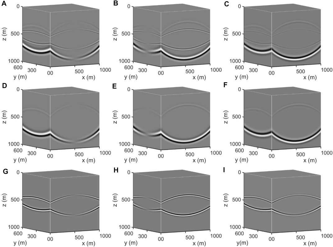
FIGURE 1. Three-component snapshots of particle velocity at 0.4 s computed based on Eq. 1. (A–C) The joint velocity components of P- and S-waves in x, y, z directions, (D–F) The P-wave components in x, y, z directions computed by applying Eq. 1, (G–I) The S-wave components in x, y, z directions computed by applying Eq. 1.

Obtaining the Poynting Vector of Pure P- and S-Waves in the Reverse-Time Extrapolation

According to the definition of the Poynting vector in seismic wavefield (Yoon and Marfurt, 2006), the following equations can be used to calculate the Poynting vector of pure P- and S-waves in the wavefield extrapolation using Eq. 1 (Tang et al., 2016):

$\begin{array}{c}\{\begin{array}{c}{\mathit{E}}_{\mathit{P}}=-\theta {\mathit{v}}_{\mathit{P}}\\ {\mathit{E}}_{\mathit{S}}=-{\mathit{v}}_{\mathit{S}}\times \mathit{\omega }\end{array}\end{array}(2)$

where ${\mathit{E}}_{\mathit{P}}$ and ${\mathit{E}}_{\mathit{S}}$ are P-wave and S-wave Poynting vectors, respectively.

Since Eq. 1 explicitly contains parameters needed in Eq. 2, it is convenient to obtain the Poynting vector of P-wave and S-wave in the reverse-time extrapolation of the receiver-wavefield by applying Eq. 1, and further obtain the propagation directions of pure P- and S-waves at each imaging point for each timestep (Tang et al., 2016). The wavefield can be separated into pure P- and S-wavefields of different propagation directions simultaneously during the imaging.

To verify the advantages mentioned above, we take the three-layer model shown in Figure 2 to calculate the forward extrapolated Poynting vector of source-wavefield based on the first-order velocity-stress equations and the first-order velocity-dilatation-rotation equations, respectively. The model is the size of 2000 × 2000 m, and the grid size is 5 × 5 m. The absorbing boundaries are implied by PML with 100 layers. The P-wave velocity model is shown in Figure 2, and the corresponding S-wave velocity model is computed from $c_P$ with a ratio of $\frac{c_P}{c_S}=1.73$. The P-wave source is a Ricker wavelet with a dominant frequency of 35 Hz located in the middle of the surface (1,000 m, 0 m). The time-stepping interval is 0.5 ms. In Figure 3, we show the difference of the Poynting vectors obtained from velocity-stress equations (Figure 3A) and velocity-dilatation-rotation equations (Figure 3B for P-wave and Figure 3C for S-wave). The first-order velocity-stress equations notably can only get the Poynting vector of the mixed P- and S-wavefields as shown in Figure 3A. When P- and S-waves exist simultaneously at a certain imaging point, the Poynting vector is neither that of P-wave nor that of S-wave (for example, indicated by the black circle in Figure 3A). Apparently, it is not easy to accurately distinguish the propagation directions of pure P-wave and pure S-wave based on this vector. In contrast, the Poynting vector of pure P-wave and pure S-wave can be obtained by applying the velocity-dilatation-rotation equations (Figure 3B,C), which can accurately describe the propagation directions of a particular type of wave.

FIGURE 2

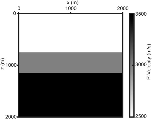
FIGURE 2. The three-layer horizontal P-wave velocity model. The P-wave velocities of the three layers from top to bottom are 2,500, 3,000, and 3,500 m/s, respectively. The depths of the two interfaces are 750 and 1,150 m, respectively.

FIGURE 3

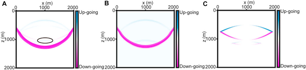
FIGURE 3. Comparisons of Poynting vector snapshots for the velocity-stress equations and velocity-dilatation-rotation equations at 0.495 s. Blue represents the up-going wave and pink represents the down-going wave, respectively. (A) A snapshot of the z-component of the Poynting vector using the velocity-stress equations. The black ellipse indicates locations that P- and S-waves exist simultaneously. (B) A snapshot of the z-component of the Poynting vector of the P-wave using the velocity-dilatation-rotation equations. (C) A snapshot of the z-component of the Poynting vector of the S-wave using the velocity-dilatation-rotation equations.

Once the Poynting vector of P-wave and S-wave are calculated in wavefield extrapolation, the wavefield can be separated into wavefields propagating in different directions. The formulas for separating P-wave into waves of opposite propagation directions are given by:

$\begin{array}{c}\begin{array}{c}{\mathit{P}}^{+}\left(x,y,z,t\right)=\{\begin{array}{cc}0& E_P^i\ge 0\\ \mathit{P}\left(x,y,z,t\right)& E_P^i<0\end{array}\\ {\mathit{P}}^{-}\left(x,y,z,t\right)=\{\begin{array}{cc}\mathit{P}\left(x,y,z,t\right)& E_P^i\ge 0\\ 0& E_P^i<0\end{array}\end{array}\end{array}(3)$

where $\mathit{P}\left(x,y,z,t\right)$ is the vector P-wave at the position (x, y, z) at time $t$, which represents the ${\mathit{v}}_{\mathit{P}}$ in the velocity-dilatation-rotation equations. ${\mathit{E}}_{\mathit{P}}={\displaystyle \sum _{i=x,y,z}{E}_p^i}$, where $E_P^i$ is the $i$-component of P-wave Poynting vector, and $i$ represents the multi-component of the P-wave. $+$ and $-$ represent the opposite directions of waves in the $i$-component, respectively. When $\mathit{i}=z$, ${\mathit{P}}^{+}\left(x,y,z,t\right)$ and ${\mathit{P}}^{-}\left(x,y,z,t\right)$ represent the up- and down-going waves in the z-component of the P-wave, respectively. The formulas for S-wave separation are analogous to Eq. 3, with the Poynting vector of the P-wave replaced by that of the S-wave. And the other two components are separated in the same way as the z-component.

Imaging Condition

The cross-correlation of source- and receiver-wavefields is commonly used in the ERTM using P- and S-waves (Yan and Sava, 2008; Du et al., 2012b) with the following basic ideas. 1) Calculating the divergence of the source-wavefield to obtain the pure P-wave $\left(S_P\right)$ component of the source-wavefield, and calculating the divergence and curl of the receiver-wavefield to obtain the pure P-wave $\left(R_P\right)$ and the pure vector S-wave $\left({\mathit{R}}_{\mathit{S}}\right)$ of the receiver-wavefield (Dellinger and Etgen, 1990). 2) Applying $R_P$ and $S_P$ to perform zero-time-delay cross-correlation and stack to get the reflected wave migration image. 3) Realizing the scalarization of ${\mathit{R}}_{\mathit{S}}$ (Du et al., 2014) and performing zero-time-delay cross-correlation with $S_P$ to obtain the converted-wave migration image. The above imaging methods are robust to noise existence (Xue, 2013) and with clear physical meanings of the imaging results. However, the scalarization of the vector S-wave will lose its vector properties. In addition, many challenging problems in the vector S-wave scalarization technique are still not resolved. For example, when the structure is complex, the polarity of the S-wave is challenging to obtain accurately. The inaccurate polarity correction will cause local fragmentation in the migration image.

To overcome the above problems, Wang and He (2017) proposed the cross-correlation imaging condition of vector wavefield dot product based on the separation of traveling waves. It first calculates the gradient and curl of the scalar P-wave and the vector S-wave respectively by the divergence and curl operators to obtain the P- and S-waves of the vector potential. Then, it uses the Poynting vector to separate P- and S-waves of the vector potential to acquire waves of the different propagation directions. Finally, the cross-correlation imaging is carried out by using the source- and receiver-wavefields of the opposite propagation directions to obtain P- and S-waves migration results. Their method does not require the scalarization of the vector S-wave, and the vector properties of the S-wave remain during the imaging process. Moreover, it is not necessary to employ polarity correction for the converted-wave migration result.

Although the imaging conditions mentioned above can often achieve promising imaging results for active source multi-component seismic data, they are not suitable for passive source data that lack accurate source information and cannot enable the extrapolation of the source-wavefield. Furthermore, it is difficult for the active source data to provide an accurate source wavelet for the wavefield extrapolation when the spectra of the multi-component seismic recording are inconsistent. The incorrect source wavelet will often result in large position errors in migration results. Xiao and Schuster (2009) proposed the passive source imaging condition for VSP imaging. The source-free imaging condition helps avoid the overburden effects and results in a better image of the salt flank by the receiver data. Shang et al. (2012) and Shabelansky et al. (2015) argued that passive seismic without location information can be used to achieve the source-free subsurface image. Based on the relationship between the P-wavefield and converted S-wavefield in the receiver extrapolation, Shabelansky et al. (2017) demonstrated a source-free converted-wave RTM imaging condition, which only uses the back-propagation P- and S-waves to perform cross-correlation imaging. As a result, it does not require source extrapolation, thereby saving calculation time and storage resources for source-wavefield reconstruction.

In this study, we apply the vector imaging condition to the RTM of the first-order velocity-dilatation-rotation elastic wave equations. First, we take advantage of velocity-dilatation-rotation equations to obtain the P-wave and S-wave with different propagation directions. There is no need for the explicit decomposition of the P- and S-waves. We can accurately obtain the propagation directions of pure P- and S-waves, assuming that there is only one set of P-wave and S-wave on the same imaging point at the same time. Then, based on the idea of vector dot product cross-correlation, we present a more precise source-free P-SV converted-wave imaging condition.

Shabelansky et al. (2017) gave a source-free converted-wave imaging condition:

$\begin{array}{c}{I}_{PS\left(x,y,z\right)}=\frac{{\displaystyle {\sum }_0^{t_{max}}{\mathit{P}}_R\left(x,y,z,t\right){\mathit{S}}_R\left(x,y,z,t\right)}}{{\displaystyle {\sum }_0^{t_{max}}{\mathit{P}}_R^2\left(x,y,z,t\right)}}\end{array}(4)$

where $I_{PS }$ is the converted-wave migration result, ${\mathit{P}}_R$ and ${\mathit{S}}_R$ are the P-wavefield and the converted S-wavefield of the receiver, respectively. $t$ represents time, and $t_{max}$ is the maximum recording length, and x, y, z are the three spatial coordinates of the rectangular coordinate system.

To improve the stability and amplitude fidelity of Eq. 4, Shabelansky et al. (2017) further modified it as follows:

$\begin{array}{c}{I}_{PS\left(x,y,z\right)}=\frac{{\displaystyle {\sum }_0^{t_{max}}4{\mathit{P}}_R\left(x,y,z,t\right){\mathit{S}}_R\left(x,y,z,t\right)}}{{\displaystyle {\sum }_0^{t_{max}}\left({\mathit{P}}_R^2\left(x,y,z,t\right)+2\left|{\mathit{P}}_R\left(x,y,z,t\right){\mathit{S}}_R\left(x,y,z,t\right)\right|+{\mathit{S}}_R^2\left(x,y,z,t\right)\right)}}\end{array}(5)$

Eq. 5 represents a source-free imaging condition, which does not need to calculate, store, and reconstruct the source-wavefield, know the source position, and set the source wavelet.

When there is only one subsurface reflection interface, the imaging result of Eq. 5 represents the ratio of the S-wave reflection coefficient to the P-wave reflection coefficient in the case of P-wave incidence. However, when there are multiple subsurface reflection interfaces, due to the influence of the interlayer multiple reflections or conversions, the imaging result of Eq. 5 fails to indicate the reflection coefficient ratio of S-wave and P-wave accurately. Therefore, if only the up-going waves in the receiver-wavefield are used for the cross-correlation operation during the imaging process, the influence of the multiple reflections and conversions on the imaging results can be reduced, and the migration accuracy can be improved. Consequently, we modified Eq. 5 as follows:

$I_{PS\left(x,y,z\right)}=\frac{{\displaystyle {\sum }_0^{t_{max}}4{\mathit{P}}_R^u\left(x,y,z,t\right){\mathit{S}}_R^u\left(x,y,z,t\right)}}{{\displaystyle {\sum }_0^{t_{max}}\left({\mathit{P}}_R^u\left(x,y,z,t\right){\mathit{P}}_R^u\left(x,y,z,t\right)+2\left|{\mathit{P}}_R^u\left(x,y,z,t\right){\mathit{S}}_R^u\left(x,y,z,t\right)\right|+{\mathit{S}}_R^u\left(x,y,z,t\right){\mathit{S}}_R^u\left(x,y,z,t\right)\right)}}(6)$

where the superscript $u$ represents the up-going wavefield of the receiver.

Numerical Tests

Two-Dimensional Marmousi2 Elastic Model

To demonstrate the effectiveness of our method, we test it with the synthetic multi-component seismic data of the partial Marmousi2 model (Martin et al., 2006). The model is of the size of 6,500 × 3,505 m with a spatial grid of $\Delta x=\Delta z=5$ m. It was stimulated by the finite-difference method with the 100-layer PML absorbing boundaries. We generate 100 P-wave sources located at a depth of 5 m below the sea surface with a horizontal interval of 65 m using a Ricker wavelet with a dominant frequency of 35 Hz. We compute the synthetic seismogram up to 4 s length with the time-stepping interval of 0.5 ms. The receiver array is located on the seafloor at 455 m depth, with a total of 1,300 traces and an interval of 5 m. The first shot is at the coordinate of $x=0$ m. The receiver array is fixed, and the shots roll one by one. Consequently, we can obtain the multi-component synthetic seismogram of 100 shots.

Figure 4 shows the RTM images obtained by using different equations and imaging conditions. Figure 4A and Figure 4B both use the first-order velocity-stress equations with the cross-correlation imaging condition of the source- and receiver-wavefields applied. The difference between the two is that Figure 4B performs wavefield separation according to the propagation directions of P- and S-wavefields before cross-correlation imaging, and then only wavefields with opposite propagation directions are involved in imaging, while Figure 4A allows all wavefields of the same or different propagation directions in P- or S-wavefields to be used in imaging. Figure 4A does not separate the directions of P-and S-wavefields, resulting in stronger low-wavenumber imaging artifacts than Figure 4B. The migration image of Figure 4C is obtained by decomposing the wavefield into the P-wavefield and S-wavefield, and separating the propagation directions of the P-wavefield and S-wavefield based on the velocity-dilatation-rotation equations, and applying the source-free imaging condition. There is no impact of source extrapolation, and the method we proposed shows a high imaging accuracy and a larger imaging range (Figure 4C).

FIGURE 4

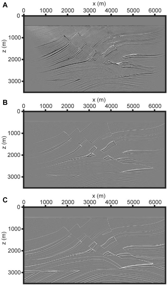
FIGURE 4. (A) The migration image of the cross-correlation imaging conditions without wavefield decomposition and wavefield separation, using the first-order velocity-stress equations. (B) The migration image of the cross-correlation imaging condition with wavefield separation, using the first-order velocity-stress equations. (C) The migration image uses the imaging condition of Eq. 6 and the elastic wave equations of Eq. 1.

Since the first-order velocity-stress elastic wave equations can only obtain the Poynting vector of the mixed wavefield, the vector can only acquire the propagation directions of the mixed wavefield, rather than that of the pure P-wave or the pure S-wave. However, the propagation directions of mixed wavefield are not consistent with that of pure P-wave or pure S-wave. Therefore, using mixed wavefield propagation directions to correct the S-wave polarity may result in incorrect polarity, lower quality of migration images, unclear structure, and destruction of the event continuity in the migration image. On the contrary, the Poynting vector of P-wave and S-wave obtained by the first-order velocity-dilatation-rotation equations can accurately represent P- and S-wave propagation directions, respectively. In turn, more accurate P-SV converted-wave migration results can be obtained.

In terms of computational efficiency, the source-free converted-wave imaging condition does not need source-wavefield extrapolation, storage, and reconstruction, which dramatically decreases the calculation cost and temporary file storage amount. Using one-shot migration of the model shown in Figure 5 as an example, the calculation time of source-free converted-wave imaging condition is more than 2.5 times faster than that of conventional cross-correlation imaging condition under the same hardware condition.

FIGURE 5

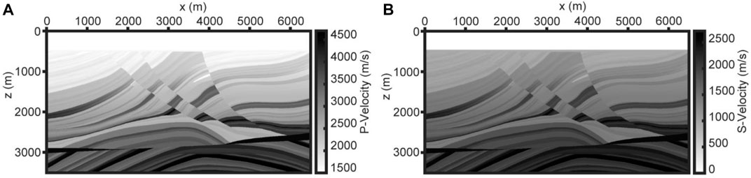
FIGURE 5. Partial Marmousi2 velocity models of (A) P-wave and (B) S-wave.

Three-Dimensional SEG/EAEG Salt Model

We also test our method on a 3D SEG/EAEG salt model as shown in Figure 6. The model is of the size of 3,000 × 3,000 × 2,010 m, with the spatial grid of $\Delta x=\Delta y=\Delta z=10$ m. The PML absorbing boundaries are set to 30 layers. The time-stepping interval is 0.35 ms. We generate P-wave sources located at 10 m depth, using the Ricker wavelet with a dominant frequency of 35 Hz. A total of seven shot lines are set up with a line interval of 400 m. Each shot line is generated from the left of the model with a shot interval of 100 m. There are 30 shots in each shot line, for a total of 210 shots. The data is recorded by 151 multi-component receiver lines located on the ground with the receiver line interval of 20 m. There are 301 traces at the group interval of 10 m on each receiver line. During the data acquisition process, the shot is moved while the receiver array remains fixed.

FIGURE 6

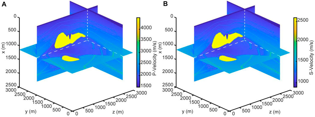
FIGURE 6. Partial SEG/EAEG salt velocity models of (A) P-wave and (B) S-wave.

The converted-wave migration image that uses the imaging condition proposed in this study (Figure 7B) is clearer and more accurate than the vector field dot product cross-correlation (Wang and He, 2017) migration image (Figure 7A) in the three-dimensional case. Figure 7B can accurately utilize subsurface media with no obvious low-wavenumber imaging artifacts in the migration image. The interfaces in the migration image are continuous. The correct subsurface structure and the geological interface can be observed. The improvements both in the accuracy and resolution of the image further demonstrate the imaging ability of our method.

FIGURE 7

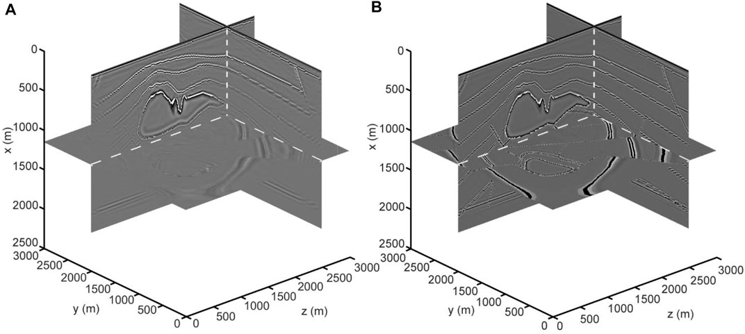
FIGURE 7. (A) The migration image using the vector field dot product cross-correlation imaging condition by Wang and He (2017). (B) The migration image using the imaging condition of Eq. 6. Both two migration images use the first-order velocity-dilatation-rotation equations.

Advantage Analysis

The first-order velocity-dilatation-rotation elastic wave equations can realize the automatic decoupling of the P- and S-waves, accurately indicate the propagation directions of the P-wave and S-wave, and further suppress the low-wavenumber imaging artifacts. The migration image obtained by source-free converted-wave imaging condition shows less low-wavenumber imaging artifacts and more continuous horizons, and therefore potentially more accurate images of the subsurface.

The method proposed in this study also has obvious advantages in computing efficiency. Taking the three-dimensional SEG/EAEG salt model shown in Figure 6 as an example, the calculation and storage cost required to migrate one-shot are shown in Table 1. Under the model shown in Figure 6, the computational cost of our method is reduced to about one-third of that of the traditional algorithm.

TABLE 1

TABLE 1. Comparison of the migration computational efficiency of the one-shot between the velocity-stress equations and velocity-dilatation-rotation equations.

Discussion

The converted-wave imaging method in this paper relies on an assumption: the source of multi-component exploration only excites the P-wave, while all the S-wave in multi-component recordings is converted from the P-wave. When the measured data does not meet this assumption (i.e., the excitation source excites P-wave and S-wave at the same time), it is necessary to develop a new approach to utilize the reflected S-wave and converted S-wave, and this method is no longer suitable. This algorithm also relies on the assumption that there is only one set of P-wave or S-wave at one imaging point at the same time, therefore when multiple sets of the P-wave or the S-wave are present at a certain imaging point at the same time, potential errors would be generated by our method.

The method in this paper can only be used for the P-SV converted-wave RTM, but the process of multi-component seismic data includes the imaging of both converted-wave and reflected P-wave. Therefore, the imaging results can be further improved by combining our method with the application of the acoustic RTM method for reflected P-waves.

Conclusion

We present a P-SV converted-wave RTM method based on the first-order velocity-dilatation-rotation elastic wave equations and the source-free imaging condition. It has the following advantages. 1) It is suitable for multi-component data imaging of both active- and passive-sources. 2) The ERTM computational cost is reduced to one-third of the conventional algorithm as it is no longer necessary to calculate, store and reconstruct the source-wavefield. 3) The first-order velocity-dilatation-rotation elastic wave equations include both a scalar P-wave parameter and a parameter for particle vibration velocity vector caused by dilatation motion. Therefore, the proposed algorithm can handle both pressure and three-component particle velocity data.

Data Availability Statement

The raw data supporting the conclusions of this article will be made available by the authors, without undue reservation.

Author Contributions

BH developed the idea for the study, BH, XY, and XS performed the research, BH and XY wrote the manuscript. The three authors are the executors of the specific work and contribute to the manuscript.

Funding

The research was financially supported by the National Natural Science Foundation of China (No. 41674118) and the Fundamental Research Funds for the Central Universities of China (No. 201964017).

Conflict of Interest

The authors declare that the research was conducted in the absence of any commercial or financial relationships that could be construed as a potential conflict of interest.

Publisher’s Note

All claims expressed in this article are solely those of the authors and do not necessarily represent those of their affiliated organizations, or those of the publisher, the editors and the reviewers. Any product that may be evaluated in this article, or claim that may be made by its manufacturer, is not guaranteed or endorsed by the publisher.

References

Bao, H., Li, M., and Zhang, M. (2021). Efficient Implementation of Wave-Equation Reverse Time Migration Based on Large Memory Nodes. Geophy. Prosp. Petrol. 60 (5), 732–737. doi:10.3969/j.issn.1000-1441.2021.05.004

CrossRef Full Text | Google Scholar

Bian, D., Wang, X., Yang, W., Yang, Z., and Wang, J. (2017). 3D Converted Wave Imaging. OGP 52 (Suppl. 2), 91–97. doi:10.13810/j.cnki.issn.1000-7210.2017.S2.016

CrossRef Full Text | Google Scholar

Biot, M. A. (1956). Theory of Propagation of Elastic Waves in a Fluid-Saturated Porous Solid. I. Low-Frequency Range. The J. Acoust. Soc. America 28 (2), 168–178. doi:10.1121/1.1908239

CrossRef Full Text | Google Scholar

Chang, W. F., and McMechan, G. A. (1994). 3-D Elastic Prestack, Reverse-Time Depth Migration. Geophysics 59 (4), 597–609. doi:10.1190/1.1443620

CrossRef Full Text | Google Scholar

Chattopadhyay, S., and McMechan, G. A. (2008). Imaging Conditions for Prestack Reverse-Time Migration. Geophysics 73 (3), S81–S89. doi:10.1190/1.2903822

CrossRef Full Text | Google Scholar

Claerbout, J. F. (1971). Toward a Unified Theory of Reflector Mapping. Geophysics 36, 467–481. doi:10.1190/1.1440185

CrossRef Full Text | Google Scholar

Clapp, R. G. (2009). “Reverse Time Migration with Random Boundaries,” in SEG Technical Program Expanded Abstracts 2009 (Houston, United States: Society of Exploration Geophysicists), 2809–2813. doi:10.1190/1.3255432

CrossRef Full Text | Google Scholar

Dellinger, J., and Etgen, J. (1990). Wave-field Separation in Two-Dimensional Anisotropic media. Geophysics 55 (5), 914–919. doi:10.1190/1.1442906

CrossRef Full Text | Google Scholar

Dong, L., Ma, Z., and Cao, J. (2000a). A Study on Stability of the Staggered-Grid High-Order Difference Method of First-Order Elastic Wave Equation. Chin. J. Geophys. 43 (6), 411–419. (in Chinese). doi:10.1002/cjg2.107

CrossRef Full Text | Google Scholar

Dong, L., Ma, Z., Cao, J., Wang, H., Geng, J., Lei, B., et al. (2000b). A Staggered-Grid High-Order Difference Method of One-Order Elastic Wave Equation. Chin. J. Geophys. 43 (3), 411–419. (in Chinese). doi:10.1002/cjg2.107

CrossRef Full Text | Google Scholar

Du, Q., Gong, X., Zhu, Y., Fang, G., and Zhang, Q. (2012a). “PS Wave Imaging in 3D Elastic Reverse-Time Migration,” in SEG Technical Program Expanded Abstracts 2009 (Houston, United States: Society of Exploration Geophysicists). doi:10.1190/segam2012-0107.1

CrossRef Full Text | Google Scholar

Du, Q., Zhu, Y., and Ba, J. (2012b). Polarity Reversal Correction for Elastic Reverse Time Migration. Geophysics 77 (2), S31–S41. doi:10.1190/geo2011-0348.1

CrossRef Full Text | Google Scholar

Du, Q., Gong, X., Zhang, M., Zhu, Y., and Fang, G. (2014). 3D PS-Wave Imaging with Elastic Reverse-Time Migration. Geophysics 79 (5), S173–S184. doi:10.1190/geo2013-0253.1

CrossRef Full Text | Google Scholar

Du, Q., Gong, X., Guo, C., Zhao, Q., Wang, C., and Li, X.-y. (2017). Vector-based Elastic Reverse Time Migration Based on Scalar Imaging Condition. Geophysics 82 (2), S111–S127. doi:10.1190/GEO2016-0146.1

CrossRef Full Text | Google Scholar

He, B., and Zhang, H. (2006). Vector Prestack Depth Migration of Multi-Component Wavefield. OGP 41 (4), 369–374. doi:10.3321/j.issn:1000-7210.2006.04.003

CrossRef Full Text | Google Scholar

Liu, F., Zhang, G., Morton, S. A., and Leveille, J. P. (2011). An Effective Imaging Condition for Reverse-Time Migration Using Wavefield Decomposition. Geophysics 76 (1), S29–S39. doi:10.1190/1.3533914

CrossRef Full Text | Google Scholar

Martin, G. S., Wiley, R., and Marfurt, K. J. (2006). Marmousi2: An Elastic Upgrade for Marmousi. The Leading Edge 25 (2), 156–166. doi:10.1190/1.2172306

CrossRef Full Text | Google Scholar

Murphy, W. F. (1982). Effects of Partial Water Saturation on Attenuation in Massilon sandstone and Vycor Porous Glass. J. Acoust. Soc. America 71 (6), 1458–1468. doi:10.1121/1.387843

CrossRef Full Text | Google Scholar

Poynting, J. H. (1884). XV. On the Transfer of Energy in the Electromagnetic Field. Phil. Trans. R. Soc. 175, 343–361. doi:10.1098/rstl.1884.0016

CrossRef Full Text | Google Scholar

Shabelansky, A. H., Malcolm, A. E., Fehler, M. C., Shang, X., and Rodi, W. L. (2015). Source-independent Full Wavefield Converted-phase Elastic Migration Velocity Analysis. Geophys. J. Int. 200 (2), 954–968. doi:10.1093/gji/ggu450

CrossRef Full Text | Google Scholar

Shabelansky, A. H., Malcolm, A., and Fehler, M. (2017). Converted-wave Seismic Imaging: Amplitude-Balancing Source-independent Imaging Conditions. Geophysics 82 (2), S99–S109. doi:10.1190/GEO2015-0167.1

CrossRef Full Text | Google Scholar

Shang, X., de Hoop, M. V., and van der Hilst, R. D. (2012). Beyond Receiver Functions: Passive Source Reverse Time Migration and Inverse Scattering of Converted Waves. Geophys. Res. Lett. 39 (15), L15308. doi:10.1029/2012GL052289

CrossRef Full Text | Google Scholar

Shen, J. (2017). Application of Multi-Card GPU in 3D Elastic Wave Reverse-Time Migration (RTM). Coal Geology. China 29 (03), 65–71. doi:10.3936/j.issn.1674-1803.2017.03.14

CrossRef Full Text | Google Scholar

Stewart, R. R., Gaiser, J. E., Brown, R. J., and Lawton, D. C. (2003). Converted-wave Seismic Exploration: Applications. Geophysics 68 (1), 40–57. doi:10.1190/1.1543193

CrossRef Full Text | Google Scholar

Sun, R., McMechan, G. A., Hsiao, H. H., and Chow, J. (2004). Separating P- and S-Waves in Prestack 3D Elastic Seismograms Using Divergence and Curl. Geophysics 69 (1), 286–297. doi:10.1190/1.1649396

CrossRef Full Text | Google Scholar

Sun, R., McMechan, G. A., Lee, C.-S., Chow, J., and Chen, C.-H. (2006). Prestack Scalar Reverse-Time Depth Migration of 3D Elastic Seismic Data. Geophysics 71 (5), S199–S207. doi:10.1190/1.2227519

CrossRef Full Text | Google Scholar

Sun, R., and McMechan, G. A. (2001). Scalar Reverse-Time Depth Migration of Prestack Elastic Seismic Data. Geophysics 66 (5), 1519–1527. doi:10.1190/1.1487098

CrossRef Full Text | Google Scholar

Tang, H.-G., He, B.-S., and Mou, H.-B. (2016). P- and S-Wave Energy Flux Density Vectors. Geophysics 81 (6), T357–T368. doi:10.1190/geo2016-0245.1

CrossRef Full Text | Google Scholar

Wang, D., Xin, K., Li, Y., Gao, J., and Wu, X. (2006). An Experimental Study of Influence of Water Saturation on Velocity and Attenuation in sandstone under Stratum Conditions. Chin. J. Geophys. 49 (3), 908–914. (in Chinese). doi:10.1002/cjg2.896

CrossRef Full Text | Google Scholar

Wang, P., and He, B. (2017). Vector Field Dot Product Cross-Correlation Imaging Based on 3D Elastic Wave Separation. OGP 52 (3), 477–483. doi:10.13810/j.cnki.issn.1000-7210.2017.03.009

CrossRef Full Text | Google Scholar

Wang, W., and McMechan, G. A. (2015). Vector-based Elastic Reverse Time Migration. Geophysics 80 (6), S245–S258. doi:10.1190/GEO2014-0620.1

CrossRef Full Text | Google Scholar

Whitemore, N. D. (1983). “Iterative Depth Migration by Backward Time Propagation,” in SEG Technical Program Expanded Abstracts 1983 (Houston, United States: Society of Exploration Geophysicists), 382–385. doi:10.1190/1.1893867

CrossRef Full Text | Google Scholar

Wu, G., and Qin, H. (2014). Elastic Reverse Time Migration in Isotropic Medium Based on Random Boundary. Prog. Geophys. 29 (4), 1815–1821. (in Chinese). doi:10.6038/pg20140444

CrossRef Full Text | Google Scholar

Xiao, X., and Schuster, G. T. (2009). Local Migration with Extrapolated VSP Green's Functions. Geophysics 74 (1), SI15–SI26. doi:10.1190/1.3026619

CrossRef Full Text | Google Scholar

Xue, D. (2013). Imaging Condition of Prestack Reverse-Time Migration. OGP 48 (2), 222–227. doi:10.13810/j.cnki.issn.1000-7210.2013.02.018

CrossRef Full Text | Google Scholar

Yan, J., and Sava, P. (2008). Isotropic Angle-Domain Elastic Reverse-Time Migration. Geophysics 73 (6), S229–S239. doi:10.1190/1.2981241

CrossRef Full Text | Google Scholar

Yan, J., and Sava, P. (2009). Elastic Wave-Mode Separation for VTI media. Geophysics 74 (5), WB19–WB32. doi:10.1190/1.3184014

CrossRef Full Text | Google Scholar

Yang, H., Ba, J., Tang, J., Nie, J., and Lu, M. (2006). Development of Conventional Geophysical Methods in Oil/gas Exploration. OGP 41 (2), 231–236. doi:10.3321/j.issn:1000-7210.2006.02.023

CrossRef Full Text | Google Scholar

Yoon, K., and Marfurt, K. J. (2006). Reverse-time Migration Using the Poynting Vector. Exploration Geophys. 37 (1), 102–107. doi:10.1071/eg06102

CrossRef Full Text | Google Scholar

Yu, F., Liu, B., Fan, J., and Li, Z. (2018). Analysis of Noise Suppression Effect of Several Angle Imaging Conditions in Reverse Time Migration. Prog. Geophys. 33 (1), 0297–0303. (in Chinese). doi:10.6038/pg2018BB0018

CrossRef Full Text | Google Scholar

Zhang, H., Feng, X., Fu, C., Sun, H., Wang, X., and Lu, Y. (2021). Noise Suppression during Elastic Reverse Time Migration in the Dip-Angle Domain Using a Convolutional Neural Network. Geophy. Prosp. Petrol. 60 (3), 376–384. doi:10.3969/j.issn.1000-1441.2021.03.003

CrossRef Full Text | Google Scholar