
95% of researchers rate our articles as excellent or good
Learn more about the work of our research integrity team to safeguard the quality of each article we publish.
Find out more
ORIGINAL RESEARCH article
Front. Earth Sci. , 07 April 2022
Sec. Geohazards and Georisks
Volume 10 - 2022 | https://doi.org/10.3389/feart.2022.743860
This article is part of the Research Topic High-Performance Computing in Solid Earth Geohazards: Progresses, Achievements and Challenges for a Safer World View all 10 articles
 Marisol Monterrubio-Velasco1*
 Jose C. Carrasco-Jimenez1
 Otilio Rojas1,2
 Juan E. Rodríguez1Andreas Fichtner3
 Josep De la Puente1
Emerging high-performance computing systems, combined with increasingly detailed 3-D Earth models and physically consistent numerical wave propagation solvers, are opening up new opportunities for urgent seismic computing. This may help, for instance, to guide emergency response teams in the wake of large earthquakes. A key component of urgent seismic computing is the early availability of source mechanism estimates, well before conventional and time-consuming moment tensor inversions are carried out and published. Here, we introduce a methodology that rapidly estimates focal mechanisms (FM) for moderate and large earthquakes (Mw > 4.0) by means of statistical and clustering algorithms. The fundamental rationale behind the method is that events of a certain size tend to be similar to other events of similar size in similar locations. In this work, two different strategies are used to provide different FM solutions: the first is based only in spatial considerations including statistical analysis, and the other one is based on a data clustering algorithm. We exemplify our methodology with six different subsets of the open-access Global Centroid Moment Tensor (GCMT) catalog. Specifically, our study datasets include events from Japan, New Zealand, California, Mexico, Iceland, and Italy, which represent six seismically active regions, with a large FM variability. Our results show a 70–85% agreement between our fast FM estimates and inversion results, depending on the particular tectonic region, dataset size, and magnitude threshold. In addition, our FM estimation strategies only spend few seconds for processing, since they are totally independent of seismic record retrieval and inversion. Albeit not meant to be a substitute for CMT inversions, our methodologies can bridge the time gap between earthquake detection and FM inversion.
Fast earthquake magnitude and focal mechanism (FM) estimates are key information for rapid emergency response applications, including urgent post-event seismic simulations. Few hours after the occurrence of a large-magnitude earthquake, these simulations aim to map ground shaking in the affected region to show areas of high intensity motion, which may host potential structural damages. An FM solution describes the fault-plane orientation and directions of principal stresses in the area where the earthquake occurred (Udias and Buforn 2017; Maeda 1992). The FM is given by three angles, two of them, the strike ϕ and dip δ angles, geometrically define the fault plane, and the third angle, the rake λ measures the direction of fault slip. Thus, an FM is used for the mathematical description of seismic sources in terms of the moment tensor (MT) equivalent body forces. The most general approach to determine an FM solution is by computing the centroid moment tensor (CMT). For moderate-to-large magnitude earthquakes, CMTs are usually obtained from waveform or spectral data inversions (Dziewonski et al., 1981; Dziewonski and Woodhouse 1983). Although, approaches to estimate earthquake location and magnitude are consolidated and extremely fast, automatic solutions for FM estimates are not always provided by the seismological agencies, or are only available at later times after waveform inversions have been completed (Tarantino et al., 2019). However, it is worth noting that significant efforts have been made towards almost real-time determination of FM (or CMT) by using different methods and algorithms. For example, Lin et al. (2019) and Melgar et al. (2012) exploit GPS networks, while other works use source inversion algorithms based on modelling of the W-phase, a very long-period phase (100–1,000 s) arriving at the same time as the P-wave (see, e.g., Duputel et al., 2012). Another approach relies on the azimuthal distribution of early P-wave peaks in displacement, velocity and acceleration traces (Tarantino et al., 2019). Moreover, several packages have been developed for automatic MT determination, such as Scisola (open-source software developed by Triantafyllis et al., 2016) or Gisola (Triantafyllis et al., 2021). Scisola is an open source Python based software for automatic MT calculation that combines two platforms, ISOLA (Sokos and Zahradnik 2008) and SeisComP3 (Weber et al., 2007). Gisola is an evolved version of Scisola that applies enhanced algorithms for waveform data filtering. However, the response times of most aforementioned techniques are constrained by the retrieval times of their input data, i.e., seismic records of the recent earthquakes (Melgar et al., 2012; Scognamiglio et al., 2010, and ref. there in). Therefore, the development of alternative approaches for fast FM estimations, independent of seismic records, may serve as temporary replacement until inversions have finished. This work explores statistical approaches, with the assistance of clustering algorithms, to estimate FM solutions for a new earthquake based on the similarity of ϕ, δ and λ with respect to past events. The historical databases are gathered by the open-access Global Centroid Moment Tensor (GCMT) catalog (GCMT, Ekström et al., 2012). As input data, our methodologies only require the hypocentral location and magnitude of the new earthquake. This information is promptly provided by different seismological agencies with a latency of few seconds after earthquake occurrence. Once triggered, our methodologies can provide FM estimates within seconds, thereby enabling real-time affectation analyses before FM inversions become available. Our results can be potentially used to add directivity information into fast shaking assessment estimates, shortly after the earthquake is recorded, because it is precise for large events which have damaging potential. The method, however, is not universal, because it behaves worse if smaller magnitude events are used. Hence it is no substitute for CMT inversion, but a provider of fast estimates.It is important to acknowledge that the methodology results not in one single best-fitting result, but in a collection of results among which is a good-fitting result. For shaking assessment (see, e.g., Wald et al., 1999, Wald et al., 2008) this is not a strong limitation, as few scenarios can be computed using all CMT estimates and the best fit can be assessed a posteriori. Last but not least, the methodology has a potential for probabilistic seismic hazard (PSHA, see e.g. Baker 2008; Mulargia et al., 2017) studies, especially those taking into account CMT information in their attenuation relationships or seismic modelling components. When populating hypothetical future earthquakes, in the so-called earthquake rupture forecast, CMTs could be estimated using our method, thus not necessarily restricting such earthquakes to mapped faults and their prescribed tectonic regimes. In fact, using catalog information (i.e. our CMT estimate) to make assessments about a hypothetical scenario is at the very core of PSHA. Nevertheless a seismic scenario computed using our CMT estimates would lack any kind of probabilistic component: it would be a deterministic scenario with associated uncertainties inherent to the CMT estimation methodology. The proposed methodology for FM estimation exploits information on hypocenters and magnitudes of catalogued neighboring events. Specifically, we employ conventional statistical analysis and the automatic DBSCAN clustering algorithm (Ester et al., 1996). To measure distance between two FM solutions, we use the Minimum Rotated Angle (MRA) metrics Kagan (2007) that quantify similarities between two double-couple (DC) sources in absolute angle degrees. It is worth noting that non-DC components, typically associated with volcanic activity and fluid-related earthquakes, are not the focus of our work because they do not typically produce large-magnitude, i.e. highly damaging, events (Stierle 2015; Wang et al., 2018). We assess the accuracy of the methodology through statistical comparisons of our FM results with published GCMT inversion solutions. For validation, we select six seismically active regions with large variability of the rupture mechanisms for the selected historical earthquakes used as estimation basis. These regions are Japan, New Zealand, California, Mexico, Iceland, and Italy.
We obtained the datasets used in this work from the GCMT catalog (Dziewonski et al., 1981; Ekström et al., 2012), available through the Searchable Product Depository (SPUD) of the Incorporated Research Institutions for Seismology (IRIS) (Trabant et al., 2012). Global Centroid-Moment-Tensors from the GCMT project at Lamont-Doherty Earth Observatory are available through SPUD within minutes after their publication. Initial quick-CMT solutions are shown and are later updated to GCMT solutions when updates arrive. At present, the GCMT catalog contains more than 40,000 earthquakes. From the queried catalog we use the Event information which includes the hypocenter location, earthquake magnitude, Date-Time UCT, faulting geometry, and the FM solution of moderate to large events with magnitude M ≥ 4.5. Is worth to highlight that in this work we only use the hypocenter location of the Event information to give the coherence of the first information registered after an earthquake occurs.
In this study, we consider six data subsets associated with six study regions: New Zealand, Japan, California, Mexico, Iceland, and Italy. Each subset is defined by the ranges of hypocentral locations, magnitudes and event times (Table 1). Figure 1 shows each regions and FM solutions, represented as beach balls. The beach ball sizes are proportional to the event magnitude.

TABLE 1. Filters applied to the GCMT database to extract six regional datasets. We list the total amount of events in each dataset. Databases have been queried from IRIS “https://ds.iris.edu/spud/momenttensor”
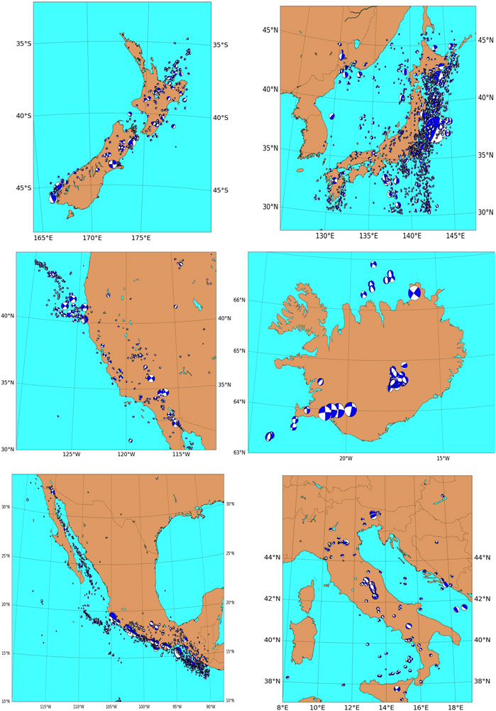
FIGURE 1. GCMT datasets used in this study (see Table 1), the epcientral locations, and the FM solutions are shown.
In this work, we assess the accuracy of our FM solutions by means of the MRA metric, proposed by Kagan (2007). This metric measures the distance between two double-couple (DC) solutions in absolute angular terms, and it enables a comparison between two DC solutions obtained by different methods, as well as variations of earthquake FMs in space and time. Moreover, the MRA has been used widely, thereby allowing us to compare methodologies of different authors.
MRA requires computing the matrix eigenvectors t, p and b, which belong to
The MRA Φ, as defined in Kagan (2007), is given by
Where t’, p’ and b’, are the eigenvectors associated to one FM solution, while a second FM solution has t”, p” and b” as eigenvectors.
Following the formulation in Kagan (2007), Eq. 2 yields the correct value of the rotation angle for Φ < 90°. However, if Eq. 2 results in Φ > 90° then a more general equation should be applied to compute Φ. For Φ > 90° to obtain the minimum rotation angle Φ Eq. 3 is applied, in those cases the smallest absolute value dot product should be negative, and the other products should be positive (further details see Kagan (2007).)
Figure 2 depicts some examples of different MRA values computed from the shown FM solutions.
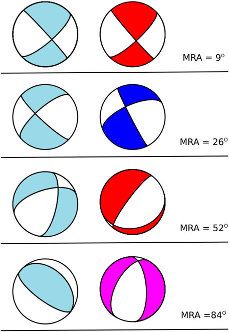
FIGURE 2. Example of the MRA metric comparing two FM solutions.
Different research results conclude that an acceptable agreement between two FM solutions is given by angle differences of the order of a few tens of degrees, while a strong variance corresponds to an angle difference greater than 50° (or 60°) (Vannucci et al., 2004; Triantafyllis 2014; Triantafyllis et al., 2016). Triantafyllis et al. (2013) found an average error between manual and the automatic FM solutions computed using Scisola of Φ ≈ 37°. Moreover, based on heuristic analyses from our statistical results, in this work we assume a similarity threshold Φth < 30°. Therefore, we suggest that two FM solutions with Φ > Φth are not comparable.
Class identification in spatial databases can be accomplished through the exploitation of clustering algorithms. Cluster analysis is developed under the assumption that spatial data has an implicit structure that can be uncovered by clustering algorithms. The clusters must comply with two characteristics: internal cohesion, also known as homogeneity, and external isolation, also known as separation. Thus, clustering techniques seek to summarize meaningfully different pattern profiles by identifying segments of points in which observations within the same cluster exhibit high degrees of similarity (homogeneity) while differing in some respects from observations in other clusters (separation). In this work, a density-based method, namely Density-based Spatial Clustering of Applications with Noise (DBSCAN) Ester et al. (1996) is used to identify geological or structural profiles, which are depicted by the clusters uncovered by the algorithm. DBSCAN relies on two parameters: a distance threshold ϵ, which indicates the maximum distance between two observations, and the minimum number of observations n to form a cluster. The first step is to describe each observation, i.e., an earthquake with a focal mechanism, using a multi-dimensional real-valued vector representation described by the hypocentral location, strike, dip and rake. The set of observations is fed to the DBSCAN algorithm to uncover the intrinsic geological or structural profiles. In order to obtain the optimal number of profiles (i.e. clusters), the distance threshold and the minimum number of samples, both of which parameters have an effect on the number of clusters. The distance threshold ϵ is estimated using the strategy based on knee/elbow methodology (Satopaa et al., 2011). And the minimum number of samples n are set equal to two
In the following subsection we provide a general description of the proposed method. Subsequently, we present its application to several regions of interest.
The proposed methodology to estimate an FM solution is based on spatial properties. Thus, once the hypocentral location of the new event with an unknown FM solution is available, we select a spherical neighborhood centered at its hypocentral location. Previous events inside this neighborhood will then be used to suggest different FM solutions. In this work we propose two different methods for this:
(a) The first method is based on spatial assumptions and uses the hypocentral Euclidean distance Δ as a metric to quantify the distance between the new event and each of its neighbors. To measure it, we apply the Haversine formula that determines the great circle distance between two points (Sinnott 1984),
Where R is the radius of the Earth, and ψ1, ψ2, and λ1, λ2 are the latitude and longitude coordinates of two points, respectively. Once d is computed, the Euclidean distance from the new event to each neighbor is given by
(b) The second method is based on the DBSCAN clustering algorithm. To apply this algorithm, we select four features, the distance from each neighbor to the hypocenter of the new event, and also the three angles of the FM of each neighbor. Once the algorithm automatically detects the clusters, we compute the position of each centroid, as well as the FM solution from the median of ϕx, δx, and λx from the events that belong to each x cluster. The number of solutions depends on the number of clusters detected in the DBSCAN algorithm. It is worth noting that a minimum number of neighbors to apply the cluster algorithm should be assumed. Hence, in this application we take a minimum of three neighbors (n = 3). The clusters automatically detected could reflect information about different regional tectonic features.
To apply the methods described in the previous subsection we follow a step-by-step process
The first step is the compilation of suitable datasets. For this, we access moment tensor information of each selected region, summarized in Table 1, through the IRIS-SPUD website 1 (Trabant et al., 2012). We perform an exploratory study to visualise the statistical FM distribution using Kaverina diagrams (Kaverina et al., 1996) which classify events according to their double-couple (DC) rupture type. Figure 3 shows the Kaverina diagrams for each study region using the visualizing tool developed in (Álvarez-Gómez 2019). Clearly dominant rupture types are observed in some regions, for example, strike-slip events in California, or normal faulting in Iceland. Other regions, such as New Zealand, Mexico and Japan, depict a larger variety of rupture types. The main purpose of visualizing historical datasets in Kaverina diagrams is to know the rupture-type at each region. This information is useful for the interpretation of results in the following section.
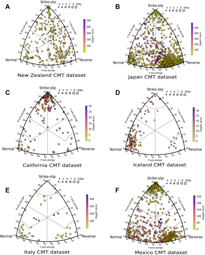
FIGURE 3. Kaverina’s diagrams for selected six regions: (A) New Zealand M ≥ 4.8, (B) Japan M ≥ 5.5, (C) California M ≥ 4.4, (D) Iceland M ≥ 4.6, (E) Italy M ≥ 4.6, and (F) Mexico M ≥ 5.5.
In the second step, we perform a statistical analyses using the two methods described in the previous subsection. This statistical evaluation aims to test the proposed methodology using each earthquake in the dataset as an independent observation, considering them as a hypothetical new event with unknown FM. Moreover, the statistical analysis allows us to quantify the accuracy of the proposed methodology by means of the MRA computed between the proposed and the original solution. In this work, we choose an MRA threshold value of Φth = 30° (Triantafyllis 2014; Kagan 2007), below which two FM solutions are deemed sufficiently similar, suggesting that the proposed one may indeed be used as a first guess for the new earthquake with unknown FM solution. This value is motivated by earlier studies on the similarity between FM solutions (Triantafyllis et al., 2013, Triantafyllis et al., 2016; Altunel and Pinar 2021), and by the observation that differences between FM solutions for an earthquake provided by different agencies are typically below Φ = 30°. From this point of view both methods described in the previous subsection can be considered supervised techniques, because the FM solution for the new-event is already known.
As previously mentioned, each method requires a minimum number of neighbors around the new event. At least three neighbors, n = 3, for the DBSCAN algorithm, and one neighbor, n = 1, for the hypocentral Euclidean distance. In the following, we will denote by Ωn the number of events in the dataset that fulfill the requirement of having a minimum of n neighbors.
In the third, step we optimize the neighborhood size. Trying to find an optimal size, we modify the radius dth of the spherical neighborhood. To find the optimum dth, we repeat the previous step, increasing the neighborhood radius after testing all the events in the dataset. We start with a radius of 20 km, and increase up to 200 km in 10 km steps. An optimum dth value must satisfy two conditions:
(1) a large number of events in the dataset with at least one neighbor inside the sphere, that is, a large Ω1,
(2) and a large percentage of events with at least one neighbor with Φ < 30°.
In Figure 4, we exemplify this search for an optimal dth. Blue bars indicate the percentage of events with at least one solution with Φ < 30°. The red triangles depict the percentage of events in the dataset considered in the analysis, i.e., events with at least one neighbor inside the sphere (Ω1). For all regions, as the neighborhood size increases, the percentage of spheres with at least one neighbor increases until an inflection point, beyond which it remains constant. We consider this inflection point as the threshold size dth. This indicates that, although the neighborhood size increases (and thus the number neighbors), the similarities between FM solutions are not further improved. Therefore, the optimal radius of the sphere maximizes both percentages at the same time, as indicated by the orange ellipse in Figure 4.
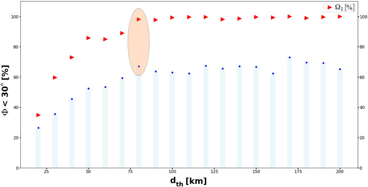
FIGURE 4. Example of the selection process of the optimal dth parameter. Red markers show the percentage of events with at least one neighbor inside the sphere (Ω1). Blue marks indicate the percentage of events with at least one FM solution with Φ < 30°. Ellipse indicates the optimum dth considered in the study as the inflection point in both curves.
To study how the minimum magnitude Mth in a dataset modifies the threshold radius dth, we repeat the same analysis considering different Mth values. However, this analysis is possible only for large catalogs, such as for the Japan and Mexico datasets. Table 2 depicts the selected dth values for each region.
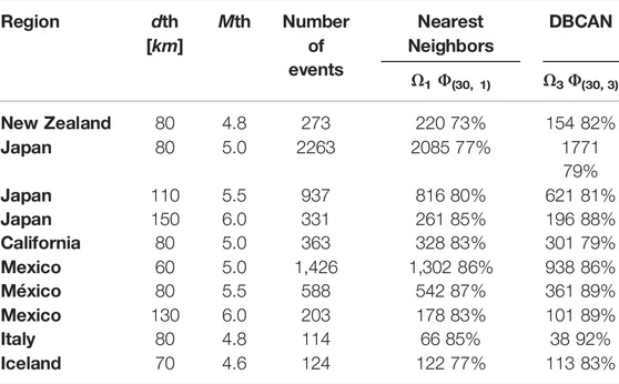
TABLE 2. Results of the methodology proposed in this work: dth is the neighborhood radius size in kilometers; Mth the minimum magnitude considered in the study; Number of events the total number of earthquakes with a magnitude larger or equal than Mth; Ω1 and Ω3 are the number of events with at least one or three neighbors inside the sphere of radius dth respectively; and
In the first part of this section we present the results of the two methods applied to the selected regions. This will be followed in the second part by specific examples for selected earthquakes in each region.
Table 2 shows the main results of the statistical analysis for each region. It is worth noting that for a similar Mth the radius dth is similar to with few tens of kilometers for different regions. Also, as Mth increases, the radius dth becomes larger. The statistical results indicate that around 70–85% of the tested events have an FM solution similar to those computed in the GCMT catalog (Φ < 30). This percentage range is accomplished for both, the clustering algorithm and the spatial metrics. Moreover in the regions with similar rupture types, such as California, Mexico, Japan or Iceland (Figure 3), this percentage increases. On the other hand, this similarity decreases in regions where the faulting types are more diverse, including New Zealand and Italy. In the datasets with few events such Italy, performance of both methods is lower because the neighborhood tends to have scarce data, thereby preventing improvements of the statistics.
Figures 5A–F shows the MRA histograms for each region, obtained with the statistical metrics (Ωth,1). We observe that the MRA distribution is clearly skewed towards low MRA values, mostly reaching Φ < 30.
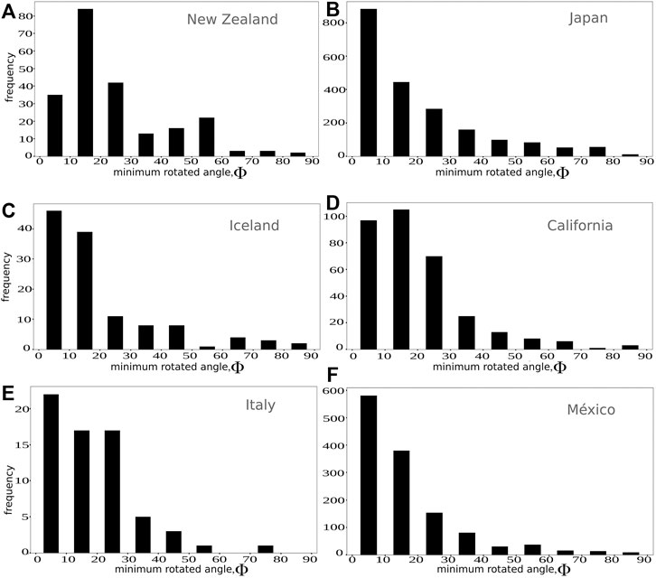
FIGURE 5. Histogram distribution of Φ values obtained by the comparison between each new event and its nearest neighbors (k1, k2, k3, k4, k median). The values represented in the plot are the minimum Φ obtained in the nearest neighbor comparison.
In Figure 6, a detailed plot shows the behavior of Φ(30, 1) considering the nearest neighbors and the median statistical solution for New Zealand. Figure 6G shows the ordered Ω values obtained in the (a-f) subplots. In dark-violet the minimum value between k1, k2, k3, k4 and k − median is depicted, from there is easy to observe how the FM solutions is improved.
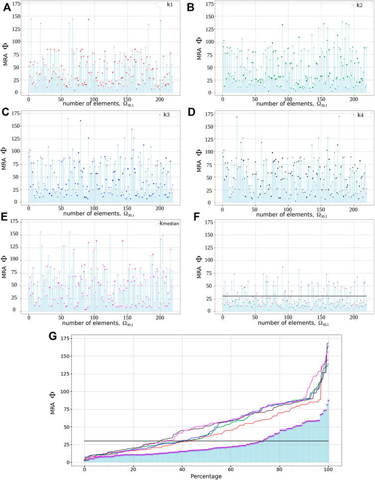
FIGURE 6. Statistical metrics results in the New Zealand region. Each subplot depicts the Φ computed for each new-event vs. the four nearest neighbors k1 (A), k2 (B), k3 (C), k4 (D), and k-Median (E). The minimum values between these five statistical solutions are depicted in subplot (F) where the horizontal line indicates the threshold Φ < 30°. (G) shows the ordered values of the other subplots in same colors except the dark-violet that corresponds to the minimum value in subplot (F).
In general, the nearest neighbor, k1, is the most likely to provide a similar FM solution. This is expected because nearby earthquakes are likely to rupture the same fault or under similar tectonic regimens. However, we also observe that the median FM solution produce MRA of Φ < 30°. In those cases, most neighbors have similar rupture types than the new-event. Moreover, in some cases, also another neighbors (k2, k3, k4), show a smaller Φ than k1. This could be related to hypocenter location uncertainties.
Statistical results of the DBSCAN algorithm are shown in Figure 7 for each region. The percentages shown in this figure consider that at least one FM solution computed using the median values in each cluster has Φ < 30°, for events with at least three neighbors (Ω3). The median FM solutions are computed by using the events belonging to each automatically detected cluster. We observe that the DBSCAN algorithm computes similar percentages to the nearest neighbors statistics for those events that fulfill the number of neighbors Ω3.
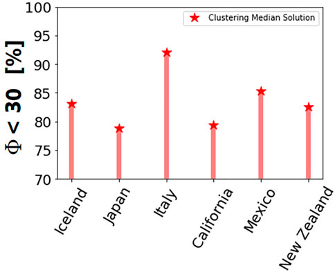
FIGURE 7. Statistical results of the DBSCAN algorithm. The percentage considers the subset Ω3 where the median FM from at least one predicted cluster has Φ < 30°.
In this section, we apply the method presented above to specific earthquakes in different regions. From the databases we randomly choose one test event with at least three neighbors inside the sphere of size dth. The selected earthquakes are listed in table 3.
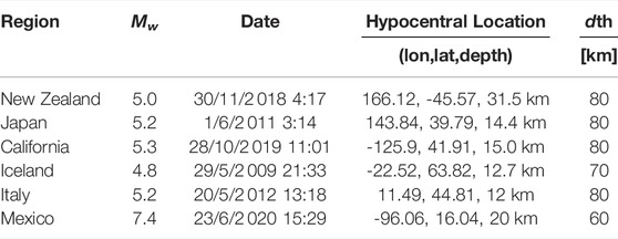
TABLE 3. Earthquakes analyzed using the statistical methodology proposed in this work (see. section 4).
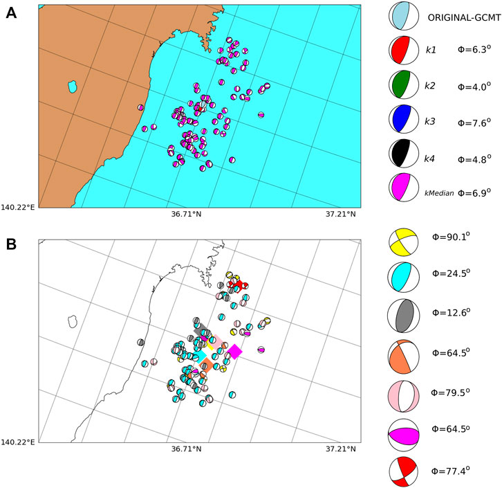
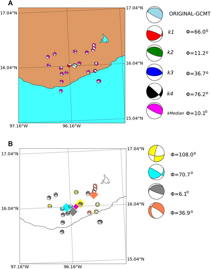
New Zealand Figure 8A shows the spatial epicentral locations and focal mechanisms of the test event, it neighbors inside the sphere, and the median event. and their focal mechanism in magenta color is plotted. The closest neighbor is shown in red. In this example, we obtain MRA values of Φ < 30° for the three nearest events k1, k2 and k3, and for the median event k − median.
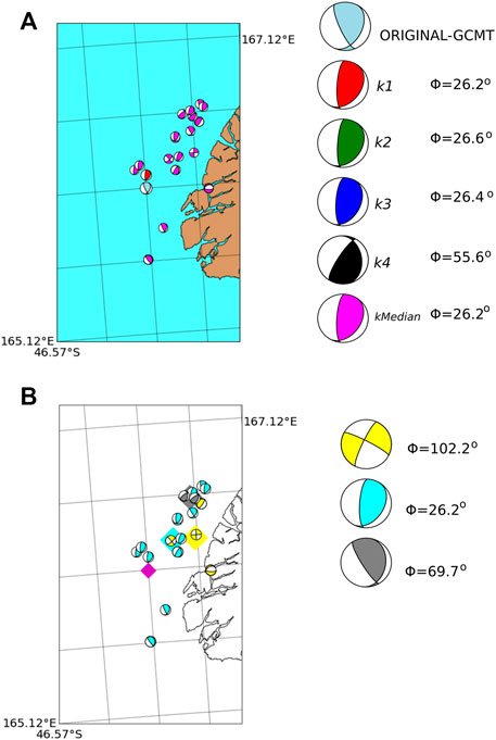
FIGURE 8. (A) Nearest neighbor solutions for a particular example in New Zealand (see Table 3). The map shows the location and focal mechanism of the test event (light-blue) and its neighbors. From closer to farther solutions, k1 (red beachball), k2 (green), k3 (dark-blue), k4 (black), and k − median (magenta). The MRA values Φ, listed to the right, measure the differences between each neighbor and the test event solution. (B) DBSCAN results for the same earthquake of Figure 8A in light-blue. The magenta diamond indicates its epicentral location. The beach balls with the same color belong to the same cluster defined by the DBSCAN algorithm. The centroids of each cluster are shown in diamond markers of the corresponding color. Those centroids are computed as the mean value of the latitude, longitude and depth from each event in the cluster. At the right side the median FM solutions computed in each cluster are shown. The MRA value Φ relative to the test-event is also indicated.
The DBSCAN clustering results are presented in Figure 8B. The different colors indicate the clusters detected in the DBSCAN algorithm and the diamonds mark their respective cluster-centroid locations. In this particular example, the smallest cluster has the more similar FM solution to the test event.
Japan The dataset of the Japan region is the largest in our analysis. We also choose randomly an earthquake with more than three neighbors inside a sphere of radius dth = 80 km size. Our threshold magnitude in this example is 5.0.
The hypocentral locations and focal mechanisms of the test event and its four nearest neighbors are displayed in Figure 9. In this example, the similarity is high for all neighbors. This is also reflected in the clustering algorithm which detects three clusters. Is worth to note that the clustering algorithm joins in the yellow cluster different event solutions. Let us keep in mind that the objective of cluster analysis is to generalize the solution model, thus, some individual events may be misclassified, which does not diminish the contribution of the solution. The generalization seeks to have good classification of spatial events in the general population of events, and low error rates do not mean perfect classification. However, it is important to note that the rest of the clusters in Figure 9 share many similarities between their elements reflecting a good clustering selection by the DBSCAN. The most similar median FM solution is for the larger cluster. These results could indicate similar geological patterns in that region, producing events with similar FM solutions.
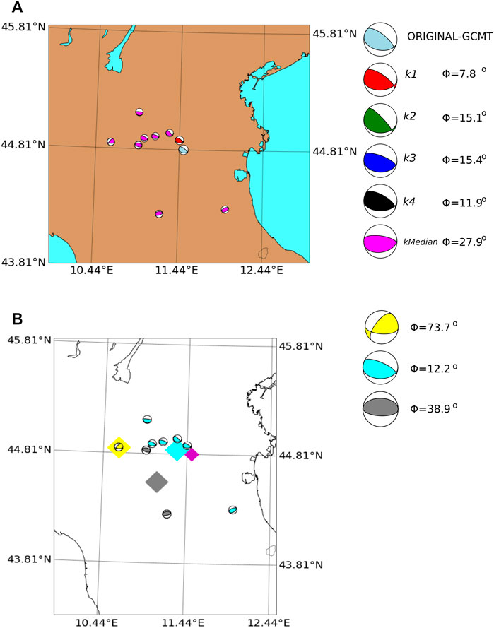
California The California region shows a predominant strike-slip rupture style, as seen in Figure 3. The results of our method, displayed in Figure 10, reveal a similarity close to Φ < 30°. In this example, the k-median is the event with the lowest MRA. The cluster analysis gives three groups, with the largest cluster being the one with the closest centroid and the smallest median MRA.
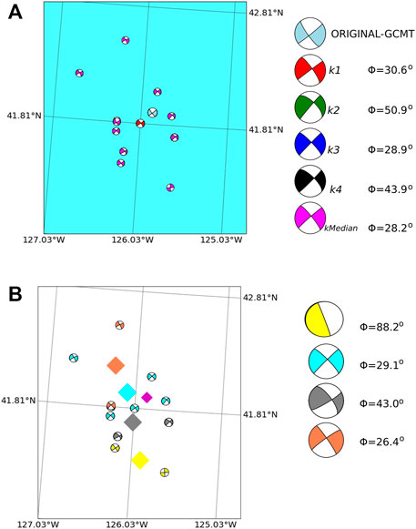
Iceland In this example, the nearest neighbors metric offers a better solution for the closest neighbor k1 (see Figure 11). The clustering results also provide a good solution for the cluster with the closest centroid to the test event, thus indicating short-range similar tectonics over distances of few kilometers).
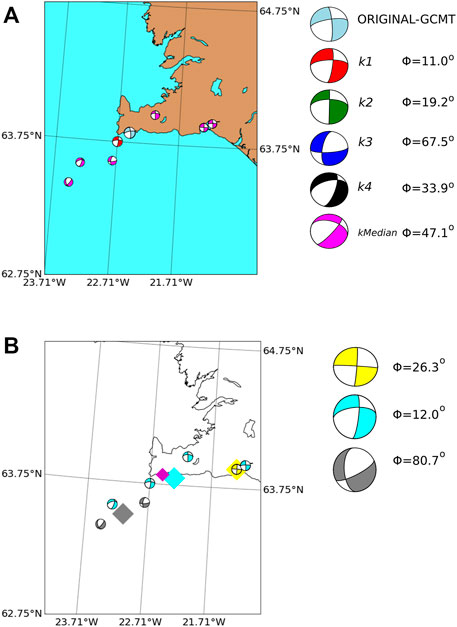
Italy The Italian region shows a predominantly normal and reverse rupture type distribution (Figure 3). However, this database has only 118 earthquakes, and so we consider all events provided in the GCMT catalog. In the example shown in Figure 12, we observe a large similarity between the selected earthquake and its neighbors, with the lowest MRA for the nearest neighbor k1. The results from the clustering algorithm also provide a similar solution for the larger cluster with the closest centroid.
Mexico The Mexican region has one of the largest datasets. The statistical results provide one event with Φ < 30°. In this particular example, we observe that the k − median neighbor gives the largest similarity (Figure 13). Moreover, the median FM of the largest cluster provides the most similar solution to the test event.
In this work we propose an inversion-free approach to the fast estimation of FM solutions, primarily intended to serve as input for urgent seismic simulations or similar problems with computation deadlines. Within this context, the rapid estimation of source parameters is highly relevant. Moreover, the predictive power of historical datasets represents an opportunity that is worth being exploited. In particular, in this work we develop a methodology for the estimation of FM solutions that is based purely on past earthquakes. After statistically validating the experiments, we find some important advantages of this statistical estimation tool.
Firstly, the method is extremely fast, with time to solution at
Among the advantages of our method, it relies on catalog information about past events. This is in contrast to more traditional methods based on waveform analysis, hence our method is significantly faster. Among its disadvantages, with respect to classical CMT inversion, we can only estimate CMT from large events, which are more likely to behave similarly to other similar events in the catalog. For smaller events our approach loses precision. Moreover, non-DC components are ignored in our study, which is not very relevant for large earthquakes but definitely relevant for smaller-event catalogs. In addition, we acknowledge that the method relies in similarity among large earthquakes recorded in a particular region. If events are few or too dissimilar, our method would fail. Nevertheless, the predictive capacity of our method can be analyzed a priori for such a region and thus we can establish the method’s suitability for the region beforehand.
As a conclusion, our method can provide with suitable CMT estimates, with statistically relevant accuracy, shortly after a large event is recorded. This enables the possibility or urgent computing of seismic hazard by means of physical simulations where directivity may be a significant component. We have tested our method in several regional contexts and analyzed its accuracy. The precision that can be attained depends strongly on the statistical distribution of large events in our study region’s catalog but produces a starting point for analysis prior to the latter determination of the CMT by means of inversion, which supersedes our result.
In future works we will study the impact of CMT accuracy in ground motion values and intensity measures such as peak ground accelerations resulting from simulations. Similarly we will analyze means to improve the method’s predictive capabilities by narrowing the choice of final CMT candidates.
Figures, tables, and images will be published under a Creative Commons CC-BY licence and permission must be obtained for use of copyrighted material from other sources (including re-published/adapted/modified/partial figures and images from the internet). It is the responsibility of the authors to acquire the licenses, to follow any citation instructions requested by third-party rights holders, and cover any supplementary charges.
The datasets presented in this study can be found in online repositories. The names of the repository/repositories and accession number(s) can be found below: http://ds.iris.edu/spud/momenttensor.
MM-V, JC-J, AF, and JP, contributed to conception and design of the study. MM-V, OR, and JR wrote the first draft of the manuscript. All authors contributed to manuscript revision, read, and approved the submitted version.
The research leading to these results has received funding from the European Union’s Horizon 2020 research and innovation programme under the grant agreement no. 823844, the Center of Excellence for Exascale in Solid Earth (ChEESE CoE Project).
The authors declare that the research was conducted in the absence of any commercial or financial relationships that could be construed as a potential conflict of interest.
All claims expressed in this article are solely those of the authors and do not necessarily represent those of their affiliated organizations, or those of the publisher, the editors and the reviewers. Any product that may be evaluated in this article, or claim that may be made by its manufacturer, is not guaranteed or endorsed by the publisher.
MM-V, JR, OR, AF, JP, thank the ChEESE CoE Project.
1https://ds.iris.edu/spud/momenttensor, last access 27/8/2020
Aki, K., and Richards, P. G. (2002). Quantitative Seismology the City. 2nd ed. Sausalito, CA: University Science Books.
Altunel, E., and Pinar, A. (2021). Tectonic Implications of the Mw 6.8, 30 October 2020 Kuşadası Gulf Earthquake in the Frame of Active Faults of Western Turkey. Turkish J. Earth Sci. 30, 436–448. doi:10.3906/yer-2011-6
Álvarez-Gómez, J. A. (2019). FMC-earthquake Focal Mechanisms Data Management, Cluster and Classification. SoftwareX 9, 299–307. doi:10.1016/j.softx.2019.03.008
Baker, J. W. (2008). An Introduction to Probabilistic Seismic hazard Analysis (Psha). White paper, 72. version 1.
Duputel, Z., Rivera, L., Kanamori, H., and Hayes, G. (2012). W Phase Source Inversion for Moderate to Large Earthquakes (1990-2010). Geophys. J. Int. 189, 1125–1147. doi:10.1111/j.1365-246x.2012.05419.x
Dziewonski, A. M., Chou, T.-A., and Woodhouse, J. H. (1981). Determination of Earthquake Source Parameters from Waveform Data for Studies of Global and Regional Seismicity. J. Geophys. Res. 86, 2825–2852. doi:10.1029/jb086ib04p02825
Dziewonski, A. M., and Woodhouse, J. H. (1983). An experiment in Systematic Study of Global Seismicity: Centroid-Moment Tensor Solutions for 201 Moderate and Large Earthquakes of 1981. J. Geophys. Res. 88, 3247–3271. doi:10.1029/jb088ib04p03247
Ekström, G., Nettles, M., and Dziewoński, A. M. (2012). The Global CMT Project 2004-2010: Centroid-Moment Tensors for 13,017 Earthquakes. Phys. Earth Planet. Interiors 200-201, 1–9. doi:10.1016/j.pepi.2012.04.002
Ester, M., Kriegel, H.-P., Sander, J., and Xu, X. (1996). A Density-Based Algorithm for Discovering Clusters in Large Spatial Databases with Noise. Kdd 96, 226–231.
Frohlich, C. (1996). Cliff's Nodes Concerning Plotting Nodal Lines for P, Sh and Sv. Seismological Res. Lett. 67, 16–24. doi:10.1785/gssrl.67.1.16
Kagan, Y. Y. (2007). Simplified Algorithms for Calculating Double-Couple Rotation. Geophys. J. Int. 171, 411–418. doi:10.1111/j.1365-246x.2007.03538.x
Kaverina, A. N., Lander, A. V., and Prozorov, A. G. (1996). Global Creepex Distribution and its Relation to Earthquake-Source Geometry and Tectonic Origin. Geophys. J. Int. 125, 249–265. doi:10.1111/j.1365-246x.1996.tb06549.x
Lin, J.-T., Chang, W.-L., Melgar, D., Thomas, A., and Chiu, C.-Y. (2019). Quick Determination of Earthquake Source Parameters from Gps Measurements: a Study of Suitability for Taiwan. Geophys. J. Int. 219, 1148–1162. doi:10.1093/gji/ggz359
Maeda, N. (1992). A Method of Determining Focal Mechanisms and Quantifying the Uncertainty of the Determined Focal Mechanisms for Microearthquakes. Bull. Seismological Soc. America 82, 2410–2429.
Melgar, D., Bock, Y., and Crowell, B. W. (2012). Real-time Centroid Moment Tensor Determination for Large Earthquakes from Local and Regional Displacement Records. Geophys. J. Int. 188, 703–718. doi:10.1111/j.1365-246x.2011.05297.x
Mulargia, F., Stark, P. B., and Geller, R. J. (2017). Why Is Probabilistic Seismic hazard Analysis (Psha) Still Used? Phys. Earth Planet. Interiors 264, 63–75. doi:10.1016/j.pepi.2016.12.002
Satopaa, V., Albrecht, J., Irwin, D., and Raghavan, B. (2011).Finding a” Kneedle” in a Haystack: Detecting Knee Points in System Behavior. In 2011 31st international conference on distributed computing systems workshops. IEEE, 166–171. doi:10.1109/icdcsw.2011.20
Scognamiglio, L., Tinti, E., Michelini, A., Dreger, D. S., Cirella, A., Cocco, M., et al. (2010). Fast Determination of Moment Tensors and Rupture History: What Has Been Learned from the 6 April 2009 L'Aquila Earthquake Sequence. Seismological Res. Lett. 81, 892–906. doi:10.1785/gssrl.81.6.892
Sokos, E. N., and Zahradnik, J. (2008). Isola a Fortran Code and a Matlab Gui to Perform Multiple-point Source Inversion of Seismic Data. Comput. Geosciences 34, 967–977. doi:10.1016/j.cageo.2007.07.005
Stierle, E. (2015). Non-Double-Couple Components in Moment Tensors of Aftershock Seismicity and Laboratory Earthquakes. Ph.D. thesis.
Tarantino, S., Colombelli, S., Emolo, A., and Zollo, A. (2019). Quick Determination of the Earthquake Focal Mechanism from the Azimuthal Variation of the Initial P-Wave Amplitude. Seismological Res. Lett.
Trabant, C., Hutko, A. R., Bahavar, M., Karstens, R., Ahern, T., and Aster, R. (2012). Data Products at the Iris Dmc: Stepping Stones for Research and Other Applications. Seismological Res. Lett. 83, 846–854. doi:10.1785/0220120032
Triantafyllis, N. (2014). Scisola: Automatic Moment Tensor Solution for SeisComP3. Master’s thesis. Patras: School of Engineering, Computer Engineering Informatics Departme.
Triantafyllis, N., Sokos, E., and Ilias, A. (2013). Automatic Moment Tensor Determination for the Hellenic Unified Seismic Network. Bull. Geol. Soc. Greece 47, 1308–1315.
Triantafyllis, N., Sokos, E., and Ilias, A. (2016). Scisola: Real-Time Moment Tensor Monitoring for Seiscomp3. Bull. Geol. Soc. Greece 50, 1120–1129.
Triantafyllis, N., Venetis, I., Fountoulakis, I., Pikoulis, E.-V., Sokos, E., and Evangelidis, C. (2021). Gisola: Real-Time Moment Tensor Computation Optimized for Multicore and Manycore Architectures. Tech. Rep. Copernicus Meetings.
Vannucci, G., Pondrelli, S., Argnani, A., Morelli, A., Gasperini, P., and Boschi, E. (2004). An Atlas of Mediterranean Seismicity. Ann. Geophys. 47.
Wald, D. J., Quitoriano, V., Heaton, T. H., Kanamori, H., Scrivner, C. W., and Worden, C. B. (1999). Trinet “Shakemaps”: Rapid Generation of Peak Ground Motion and Intensity Maps for Earthquakes in Southern california. Earthquake Spectra 15, 537–555. doi:10.1193/1.1586057
Wald, D., Lin, K.-W., Porter, K., and Turner, L. (2008). Shakecast: Automating and Improving the Use of Shakemap for post-earthquake Decision-Making and Response. Earthquake Spectra 24, 533–553. doi:10.1193/1.2923924
Wang, R., Gu, Y. J., Schultz, R., and Chen, Y. (2018). Faults and Non-double-couple Components for Induced Earthquakes. Geophys. Res. Lett. 45, 8966–8975. doi:10.1029/2018gl079027
Keywords: focal mechanism, fast-response, urgent computing, GCMT catalog, DBSCAN clustering, source parameters
Citation: Monterrubio-Velasco M, Carrasco-Jimenez JC, Rojas O, Rodríguez JE, Fichtner A and Puente JDl (2022) A Statistical Approach Towards Fast Estimates of Moderate-To-Large Earthquake Focal Mechanisms. Front. Earth Sci. 10:743860. doi: 10.3389/feart.2022.743860
Received: 19 July 2021; Accepted: 18 February 2022;
Published: 07 April 2022.
Edited by:
Alice-Agnes Gabriel, Ludwig Maximilian University of Munich, GermanyReviewed by:
Wenhuan Kuang, Southern University of Science and Technology, ChinaCopyright © 2022 Monterrubio-Velasco, Carrasco-Jimenez, Rojas, Rodríguez, Fichtner and Puente. This is an open-access article distributed under the terms of the Creative Commons Attribution License (CC BY). The use, distribution or reproduction in other forums is permitted, provided the original author(s) and the copyright owner(s) are credited and that the original publication in this journal is cited, in accordance with accepted academic practice. No use, distribution or reproduction is permitted which does not comply with these terms.
*Correspondence: Marisol Monterrubio-Velasco, bWFyaXNvbC5tb250ZXJydWJpb0Bic2MuZXM=
Disclaimer: All claims expressed in this article are solely those of the authors and do not necessarily represent those of their affiliated organizations, or those of the publisher, the editors and the reviewers. Any product that may be evaluated in this article or claim that may be made by its manufacturer is not guaranteed or endorsed by the publisher.
Research integrity at Frontiers
Learn more about the work of our research integrity team to safeguard the quality of each article we publish.