 Stephan Schennen
 Sebastian Wetterich
 Lutz Schirrmeister
 Georg Schwamborn
 Jens Tronicke1
- 1Institute of Geosciences, University of Potsdam, Potsdam, Germany
- 2Alfred Wegener Institute Helmholtz Center for Polar and Marine Research, Department of Permafrost Research, Potsdam, Germany
Ground-penetrating radar (GPR) is a popular geophysical method for imaging subsurface structures with a resolution at decimeter scale, which is based on the emission, propagation, and reflection of electromagnetic waves. GPR surveys for imaging the cryosphere benefit from the typically highly resistive conditions in frozen ground, resulting in low electromagnetic attenuation and, thus, an increased penetration depth. In permafrost environments, seasonal changes might affect not only GPR performance in terms of vertical resolution, attenuation, and penetration depth, but also regarding the general complexity of data (e.g., due to multiple reflections at thaw boundaries). The experimental setup of our study comparing seasonal differences of summertime thawed and winter- and springtime frozen active layer conditions above ice-rich permafrost allows for estimating advantages and disadvantages of both scenarios. Our results demonstrate major differences in the data and the final GPR image and, thus, will help in future studies to decide about particular survey seasons based on the GPR potential for non-invasive and high-resolution investigations of permafrost properties.
Introduction
The mean surface air temperature in the Arctic has increased from 1960 to 2019 by nearly 4°C (GISTEMP Team, 2021) and from 2006 to 2017, the average ground temperature increase across all polar and mountain permafrost regions was 0.29 ± 0.12°C (Biskaborn et al., 2019). In addition, an increase of high temperature events has been observed, while cold temperature events have declined (AMAP, 2021). In the following decades, Arctic temperatures are expected to continue rising (Meredith et al., 2019). As a consequence, frozen ground is or will be exposed to widespread thawing conditions in near future. The resulting subsidence and wetting poses a risk to infrastructure founded on yet frozen ground. Furthermore, thawing of permafrost bears the risk of greenhouse gas release, resulting in a positive feedback mechanism for climate change (e.g., Koven et al., 2015). This is particularly true for Yedoma Ice Complex (IC) deposits being a major carbon pool in the Arctic (Strauss et al., 2013, 2017).
The expected dynamics of permafrost landscape change show a demand for subsurface investigations to extrapolate permafrost sampling results from coring and exposure sites or to monitor vulnerable infrastructure bound to climate-sensitive ground. Given the vulnerability of the environment and the scale of interest, a noninvasive method with resolution capabilities at a decimeter scale is needed for subsurface permafrost investigations. A suitable geophysical tool for non-invasive imaging of subsurface structures in these regions is ground-penetrating radar (GPR). GPR is based on the emission of electromagnetic (EM) waves, and the recording of the electromagnetic energy reflected at interfaces defined by a contrast of electrical permittivity. Allowing subsurface imaging with a decimeter resolution in a non-invasive manner, GPR has found a wide field of applications addressing different problems from civil engineering, hydrology, geology, or archeology.
In periglacial regions, GPR reflection surveying has been used to investigate geomorphological features such as pingos (Yoshikawa et al., 2006), thermokarst lakes (Schwamborn et al., 2002), deposits in glacier forelands (Schwamborn et al., 2008a), and the seasonally unfrozen uppermost active layer (Schwamborn et al., 2008b; Brosten et al., 2009). Furthermore, GPR has been used to analyze infrastructure risk at polar research stations (Campbell et al., 2018; Grigoreva et al., 2020) or to monitor snowpack accumulation (Schmid et al., 2014). Dominant interfaces in the subsurface are, for example, the permafrost table below a thawed active layer, and interfaces of adjacent sedimentary units, which exhibit different ice content and, thus, resulting in different electrical material properties.
In such GPR surveys, EM energy is transmitted and recorded typically using surface-launched antennas. The radiation characteristics are strongly focused towards the subsurface half-space depending on the permittivity of the subsurface. Thus, an antenna placed on a thawed active layer will radiate more EM energy into the subsurface than an antenna on a frozen active layer. However, the increased electromagnetic attenuation within a thawed active layer and the strong reflectivity contrast at the permafrost table may hinder EM energy to propagate into deeper permafrost layers below. In contrast, a frozen active layer is characterized by less attenuation, i.e., higher electrical resistivity, and a decreased contrast in reflectivity at the bottom of the active layer. Furthermore, the EM wavefield in a thawed active layer is expected to be more complex, because a strong increase of velocity (up to a factor of five and more) at the upper and lower interface of the active layer results in wave-guide phenomena related to such a thawed layer.
In this study, we compare two 3D GPR data sets recorded across the same field site (characterized by Yedoma Ice Complex deposits) within five months under 1) frozen and 2) thawed active layer conditions in spring (April) and summer (August) 2014, respectively. We aim to point out advantages of both scenarios to guide decisions about choosing a particular survey season for specific applications of future GPR surveying in such environments.
Survey Site and Geological Background
Our survey site is a late Pleistocene Yedoma Ice Complex on Bol’shoy Lyakhovsky Island, the southern island of the New Siberian Archipelago. Figure 1 shows an aerial orthophoto of our survey site next to a scarp, representing the sharp transition to a thermo-terrace roughly 7 up to 15 m below. The individual areas surveyed in spring (April) and summer (August) 2014 are visualized as hillshade-like representations of digital terrain models (DTM). In detail, the visualization is obtained from the vertical component of the surface normals. We chose this representation 1) to apply a uniform detrending on our tilted DTM surface and 2) to point out morphological features, namely several decimeter elevated thermokarst mounds (baidzherakhs) and depressions in between. Here, bright areas represent horizontal (flat) regions, while black areas are tilted with angles ≥11.5°. Both survey areas overlap on an area of approximately 40 × 5 m (dashed rectangle in Figure 1B), that represents our study area.
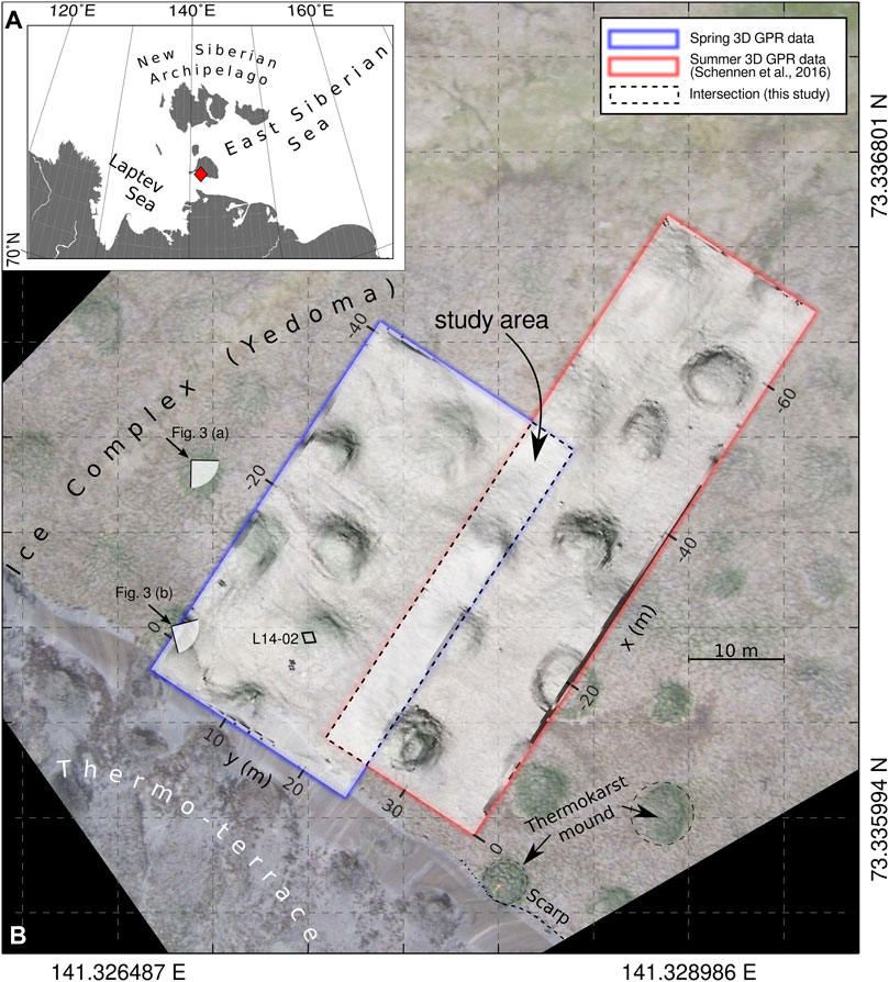
FIGURE 1. GPR survey site showing (A) the location of the study area on Bol’shoy Lyakhovsky Island and (B) an aerial orthophoto of the field site with an overlain transparent hillshade-like visualization of the digital terrain model. The dashed rectangle denotes the study area; i.e., the area where GPR data have been recorded in spring and summer 2014. The coring site L14-02 (Supplementary Table S1) is located inside the area covered by our spring GPR survey. The general elevation slope from SW to NE is −10%.
Investigations of permafrost deposits on Bol’shoy Lyakhovsky Island have been carried out since the end of the 19th century (Bunge, 1887; von Toll, 1897). Quaternary permafrost deposits were studied in the 20th century by Russian (Romanovskii, 1958a; Romanovskii, 1958b; Romanovskii, 1958c; Arkhangelov et al., 1996; Kunitsky, 1998) and by Russian-Japanese projects (Nagaoka, 1994; Nagaoka et al., 1995). Since 1999 Bol’shoy Lyakhovsky Island has been the object of several expeditions within the frame of a German-Russian science cooperation (e.g., Andreev et al., 2004, 2009, 2011; Wetterich et al., 2009, 2011, 2014, 2019, 2021; Zimmermann et al., 2017). In 2014, geophysical research of Quaternary sediments on Bol’shoy Lyakhovsky Island was carried out for the first time (Schennen et al., 2015, 2016).
The stratigraphy exposed at the southern coast of Bol’shoy Lyakhovsky Island spans discontinuously the last about 200 ka, and differentiates into ten main units. The presence of four generations of stadial and interstadial Ice Complex deposits (Tumskoy, 2012; Wetterich et al., 2019) is striking. Those are divided by thermokarst and floodplain deposits of different ages, and topped by a Holocene cover. The vertical and lateral stratigraphic contacts of the exposed units differ along the coastline depending on past climate, permafrost, and geomorphologic dynamics that defined accumulation and preservation conditions for the individual units. The stratigraphic sequence of our survey site is shown in Figure 2. In chronological order the stratigraphic units are summarised in Supplementary Table S1.
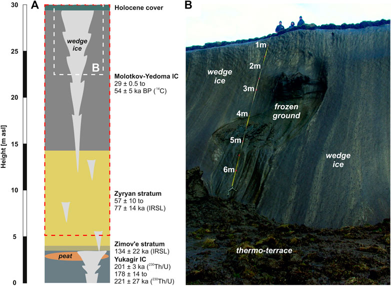
FIGURE 2. (A) Major stratigraphic sequences at our survey site as also summarized in Supplementary Table S1. The red box denotes the depth range as covered by our GPR data and the white box indicates (B) the exposed uppermost 7 m of the Holocene cover and the Yedoma Ice Complex above a thermo-terrace.
The study site chosen for the 3D GPR measurements refers to Figure 2, where the Yedoma Ice Complex of Marine Isotope Stage (MIS) 3 below the Holocene cover (MIS 1) constitutes most of the exposed permafrost. Deeper lying deposits belong to the Zyryan floodplain stratum of MIS 5–4 age, the Zimov’e stratum of MIS 6 age and the Yukagir Ice Complex of MIS 7 age (Supplementary Table S1).
Material and Methods
We acquired our 3D GPR data using a PulseEkko system from Sensors & Software equipped with a pair of unshielded 100 MHz antennas (nominal mid-frequency). To perform our survey in a kinematic manner, we mounted our antennas on a sledge and used a total tracking station (TTS, Leica TPS 1200) to track the sledge positions continuously during data acquisition (Figure 3). More details regarding this setup can be found in Böniger and Tronicke (2010). We used the same survey setup in spring (Figure 3A) and summer (Figure 3B). We recorded our data in free run mode with a line spacing of ∼25 cm and an inline trace spacing of ∼5 cm. Our data processing flow follows a standard processing sequence including zero-time-correction, bandpass filtering, gridding to a regular grid (25 cm crossline and 10 cm inline grid-point spacing), 3D topographic migration including the same amplitude scaling (Allroggen et al., 2015), and topographic correction. We used two different velocity models for migration to consider a thawed and a frozen active layer, respectively, in the data sets recorded in different seasons. For migrating our spring data, we used a uniform velocity model of v = 0.17 m/ns. For the summer data, our velocity model consists of two layers: a 40 cm thick top layer with v = 0.06 m/ns (representing the thawed active layer) and an underlying layer with v = 0.17 m/ns representing frozen ground. We extracted our velocity models from a) common-midpoint data (i.e., consequently increasing the distance between transmitting and receiving antenna, centered on a constant midpoint) and b) diffraction analysis (calculating traveltime hyperbolas and fitting these to hyperbolic diffraction patterns in the survey data). More details can be found in Schennen et al. (2016). Our TTS data processing comprised gridding on the same regular grid we used for our GPR data. We did not correct our spring TTS data for snow cover depth.
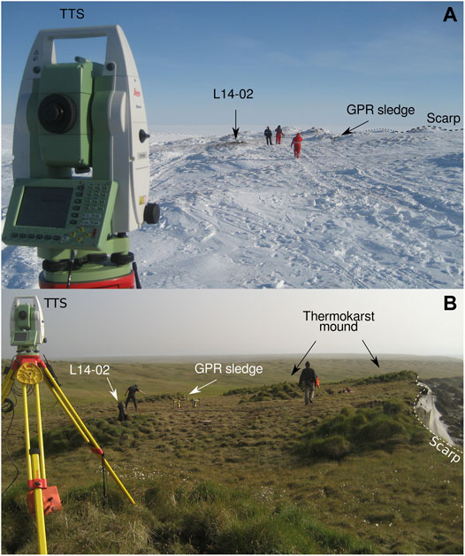
FIGURE 3. Impression of survey conditions in (A) spring and (B) summer 2014. The scarp at the southern end of our survey area represents a sharp transition to a thermo-terrace ∼7–15 m below. The coring site L14-02 (see also Supplementary Table S1) was covered by our GPR survey in spring. The viewpoints of both photos are annotated in Figure 1.
Results
With our kinematic surveying strategy tracking the GPR antenna sledge with a TTS (Böniger and Tronicke, 2010), we acquired two Digital Terrain Models (DTMs) with a spatial resolution in the order of cm. As visible in Figure 1, surface morphology of our winter DTM appears smoother compared to our summer DTM. This observation can partly be attributed to a snow cover with a thickness of up to 10 cm (see also Figure 3A) and a more slippery ground, resulting in a smoother movement of our GPR sledge. In the following, we focus on the intersecting area of both DTM and elaborate surface differences from spring to summer. Afterwards, we proceed with differences in subsurface imaging based on exemplary zoom-ins extracted from our migrated 3D GPR data sets.
Differences in Digital Terrain Model
When creating a DTM for our GPR processing flow (as needed for topographic migration and topographic correction), relative elevations within our survey area are generally sufficient. For relating our DTMs to each other, we smooth both DTMs using a 2D Gaussian kernel (standard deviation: 0.2 m, radius: 1 m) and calculate the difference height Δz = zsummer—zspring. Finally, we shift our Δz model to a mode of Δz = 0 to remove any global trend and focus on small scale topographic variations.
Figure 4A shows all grid cells of our resulting Δz model as a histogram. Because we shifted our differential DTM to quasi-equilibrium, the dominant loss of elevation is 0 cm. Some grid cells exhibit a relative elevation loss of more than 0.2 cm. Figure 4B shows a height profile that was extracted from the differential DTM illustrated in Figure 4C. The height profiles indicate an eroded thermokarst mound at the upper part of our survey area (x > −5 m) as the major region of elevation loss, as both height profiles diverge. The differential DTM below confirms that this elevation loss extends also laterally and is associated with a formerly elevated thermokarst mound at x = −3 m and y = 25 m. Grid cells that exhibit the dominant value of less than 3 cm elevation change are not bound to any particular region, but widely spread across our survey area and, thus, are interpreted to reflect the resolution capabilities of our DTM.
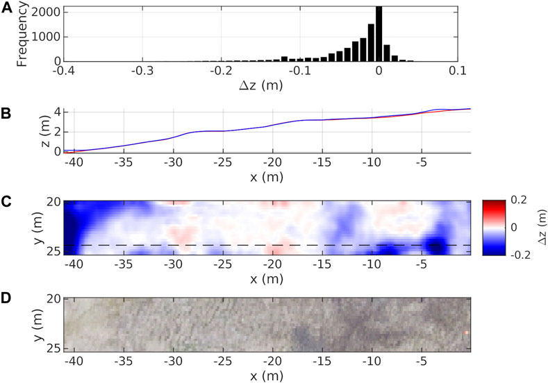
FIGURE 4. DTM elevation change from spring to summer in our study area as seen in (A) the histogram of height differences across all DTM grid cells, (B) extracted profile [dashed line in (C)] from summer DTM (red) and spring DTM (blue), (C) a map of elevation change from spring to summer 2014, (D) detail of orthophoto extracted from Figure 1.
Differences in Ground-Penetrating Radar Data
We compare our GPR data using two approaches. In the first approach (signal loss at the active-layer base), we use stacked traces before and after topographic migration for the same location to point out differences in 1D with a focus on reflectivity and absorption. In the second approach (imaging of interfaces, resolution and interpretability within 3D data), we extract exemplary 2D patches from our data sets and analyze those in time and frequency domain to investigate differences of 2D structural imaging such as those related to variations in vertical resolution and lateral continuity of reflectors. We relate our observed reflections, both between major stratigraphic units and within, to differences in ice content. According to Schwamborn et al. (2008b), these reflections can already result from a change of 30% in gravimetric ice content. Please note that all coordinates are referring to the survey grid as introduced in Figure 1.
Signal Loss at the Active-Layer Base
Figure 5 illustrates our processed GPR data including a topographic correction but without applying topographic migration. We show the same 2D line extracted from our spring data (Figure 5A) and our summer data (Figure 5B). As major differences, the summer 2D profile shows a more complex waveform pattern at traveltimes t < 60 ns (resulting from interference phenomena of antenna crosstalk and energy reflected at the active layer base) and the frozen ground below elevated areas (thermokarst mounds, see Figure 4) appears rather blind (i.e., only minor reflected energy is visible in these areas). In contrast, our spring data show a simpler early time wavefield at t < 60 ns (without dominating interference patterns) and the data provide further insights into subsurface structures within and below the thermokarst mounds. However, the spring data exhibit a more complex waveform pattern towards later traveltimes (e.g., x = −25 m, t > 210 ns) due to a higher amount of diffracted energy.
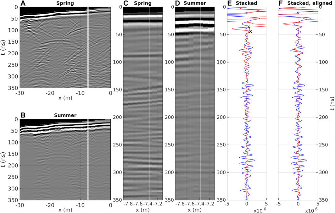
FIGURE 5. Comparison of stacked traces extracted from gridded profile data after amplitude scaling using a t2-scaling function. From left to right: 2D profile recorded (A) in spring and (B) in summer. Zoom-ins to illustrate the data used for stacking (indicated by the white box) of (C) the spring data and (D) the summer data. (E) Stacked trace of spring (blue) and summer data (red). (F) Trace-to-trace comparison after alignment at the 50 ns reflection event (see black crosses in e) resulting in a time shift of −9 ns. The shown time window of 350 ns corresponds to a depth interval of ∼30 m depth for v = 0.17 m/ns.
Based on the profiles shown in Figures 5A,B, we select a location dominated by horizontal reflections (Figures 5C,D) and calculate a median trace using five traces between x = −7.5 m ± 0.2 m as indicated by the white boxes in Figures 5A–D. Figures 5E,F shows trace-to-trace comparisons between our calculated median traces of unmigrated spring and summer data, respectively. Despite the mentioned differences at early times (t < 60 ns), the median trace of the summer data exhibits a reflection pattern similar to that of the spring data, although shifted by a lag of 9 ns as applied in Figure 5F. Exemplary ratios (summer/spring) of maximal reflection amplitudes extracted from our stacked and aligned median trace data in Figure 5F are, e.g., 0.77 (at t = 83 ns), 0.70 (at t = 107 ns), and 0.24 (at t = 234 ns), indicating an up to four times higher signal loss in summer compared to spring.
Figure 6 shows a similar illustration of the GPR data after applying the full processing flow, i.e., including 3D topographic migration before applying the topographic correction. In contrast to the unmigrated 2D profiles (Figure 5), all diffraction hyperbolas are successfully collapsed and the reflections appear smoother (Figures 6A–D). Furthermore, the trace-to-trace comparison (Figure 6E), demonstrates that the stacked traces from both data sets show already high coherency in reflection patterns below the active layer bottom (t > 60 ns) without applying an additional time shift. This observation can be interpreted as a validation of our velocity models used for the topographic migration. Here, former differences in traveltime within the unmigrated data have been corrected: i.e., diffracted energy was properly propagated back using our data set-specific rms-velocity models. Exemplary ratios (summer/spring) of maximal reflection amplitudes extracted from our migrated and stacked median trace data in Figure 5F are, for example, 0.36 (at t = 87 ns), 0.51 (at t = 110 ns), and 0.18 (at t = 234 ns), implying an up to five times higher signal loss in summer compared to spring. In comparison to the ratios delineated from unmigrated stacked traces at the same travel times, we observe typically lower ratios. We relate this observation to a more effective migration of our spring data compared to summer, where a) diffraction patterns do not occur as widespread (due to higher attenuation), and our estimated velocity model will more often deviate from reality, for example, due to small-scale contrasts in wetness, resulting in a more heterogeneous near-surface velocity field.
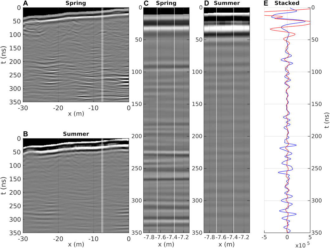
FIGURE 6. Comparison of stacked traces extracted from gridded profile data after 3D topographic migration. From left to right: 2D profile recorded (A) in spring and (B) in summer. Zoom-ins to illustrate the data used for stacking (indicated by the white box) of (C) the spring data and (D) the summer data. (E) Stacked trace of spring (blue) and summer data (red). In contrast to Figure 5E, there was no manual time shift applied, because both traces appear aligned after topographic migration. The shown time window of 350 ns corresponds to a depth interval of ∼30 m depth for v = 0.17 m/ns.
Imaging of Interfaces, Resolution and Interpretability Within 3D Data
Figure 7 compares the surroundings of an internal cryolithological reflection recorded at 120 ns (∼10.2 m depth for v = 0.17 m/ns, extracted at x = −7.5 m) from our spring data (Figure 7A) to the corresponding area extracted from our summer data (Figure 7B). Compared to the summer data, the spring data exhibit both a higher dynamic range in amplitudes and a higher vertical resolution resulting in a generally sharper image of subsurface structures. Thus, the denoted reflector appears more distinct in the spring data, while the summer data provide a smoother but less detailed image of subsurface structures which could ease reflector tracing. The corresponding amplitude spectra (Figures 7C,D) confirm these observations. Although the total amount of energy is comparable, the amplitude spectra of the summer data appear shifted towards lower frequencies and exhibit a sharper focus of energy (i.e., narrower bandwidth) compared to the spring data. This can be seen particularly in the normalized amplitude spectra shown in Figure 7D, where the summer spectrum (red) exhibits a sharp descent from ∼80 to ∼105 MHz compared to the spring spectrum (blue). As a consequence, the spring spectrum exhibits up to four times higher amplitudes around ∼110 MHz as demonstrated by the spectral ratios in Figure 7C.
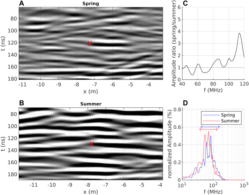
FIGURE 7. Exemplary 2D detail in time (A,B) and frequency domain (C,D). 2D data were extracted from our migrated (A) spring and (B) summer data cube (between x = −11 and −4 m, at y = 21 m), and manually aligned based on image details (red marker at center). Note, a gain factor of two has been applied to the summer data for visualization. Right column: (C) ratio of unnormalized amplitude spectra around our nominal antenna frequency and (D) normalized amplitude spectra for spring (blue) and summer (red) data. In (D), horizontal lines denote frequency range between 10th percentile A10 and 90th percentile A90 (comprising 80% of the recorded amplitudes).
Figure 8 compares the surroundings of an internal cryolithological reflection recorded at 180 ns (∼15.3 m depth for v = 0.17 m/ns, extracted at x = −17.5 m) from our spring data to the corresponding region extracted from our summer data. Both images show roughly the same dynamics in amplitude, whereas the spring data provide a slightly sharper image due to a higher vertical resolution. The summer data look smoother and miss some information from the spring data (see arrow 1 and 2 in Figure 8). In contrast to the previous example discussed in Figure 7, the seasonal difference between total recorded energy is much more distinct between spring and summer data. Again, the summer mode is shifted towards lower frequencies (∼70 MHz compared to ∼95 MHz in the spring data) and exhibits a much stronger decrease at frequencies f > 80 MHz. Normalizing both spectra to their total amplitude provides a consistent picture; i.e., the summer data exhibit a narrower shape with increased amplitude at lower frequencies (e.g., ∼0.8 at ∼70 MHz compared to 0.65 at ∼ 95 MHz).
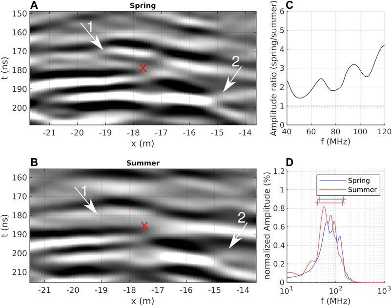
FIGURE 8. Exemplary 2D detail in time (A,B) and frequency domain (C,D). 2D data were extracted from our migrated (A) spring and (B) summer data cube (between x = −22 and −14 m, at y = 21 m), and manually aligned based on image details (red marker at center). Note, a gain factor of two has been applied to the summer data for visualization. Right column: (C) ratio of unnormalized amplitude spectra around our nominal antenna frequency and (D) normalized amplitude spectra for spring (blue) and summer (red) data. In (D), horizontal lines denote frequency range between 10th percentile A10 and 90th percentile A90 (comprising 80% of the recorded amplitudes). Arrows identify features that are further discussed in the text.
Figure 9 compares the surroundings of an internal cryolithological reflection recorded at 205 ns (∼17.4 m depth for v = 0.17 m/ns, extracted at x = −34.5 m) from our spring data to the corresponding region extracted from our summer data. Similar to Figures 7, 8, the summer image (Figure 9B) shows smoother reflection patterns than the spring image (Figure 9A). Thus, the interference around the analysis point (red marker) is not resolved and we are not able to continuously follow the black (positive) phase of the tilted reflector in the summer data (similar features are observed for other reflectors). In the spectral domain, the normalized spectra of both data sets differ less compared to the previous examples (Figure 9D). However, the spectrum of the summer data contains, across all frequencies, approximately 25% compared to the spring as demonstrated by the amplitude ratios in Figure 9C.
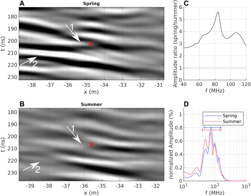
FIGURE 9. Exemplary 2D detail in time (A,B) and frequency domain (C,D). 2D data were extracted from our migrated (A) spring and (B) summer data cube (between x = −39 and −31 m, at y = 21 m), and manually aligned based on image details (red marker at center). Note, a gain factor of two has been applied to the summer data for visualization. Right column: (C) ratio of unnormalized amplitude spectra around our nominal antenna frequency and (D) normalized amplitude spectra for spring (blue) and summer (red) data. In (D), horizontal lines denote frequency range between 10th percentile A10 and 90th percentile A90 (comprising 80% of the recorded amplitudes). Arrows identify features that are further discussed in the text.
Discussion
Our three presented detailed examples show a loss of resolution from spring to summer and an increased complexity, especially, at the early travel times. In the following, we intend 1) to relate these observations to a wider assessment of the entire data cube, 2) to quantify the differences in the spectral domain, 3) to relate our observations to modeling and physics, and 4) to translate our observations into practical recommendations for future surveys.
Evaluation of Amplitude Spectra
Table 1 summarizes spectral differences between our spring and summer data for eight selected data segments. Segments 1–3 are shown in Figures 7–9, respectively. Similar to those, all segments were manually selected and cover the surrounding of distinct reflections in our 3D data. The lateral and vertical position was aligned by visual inspection. Our previous observations of an increased amplitude and resolution in the spring data is confirmed throughout all segments; i.e., the energy ratio (spectral energy in spring related to summer) varies between 1.2 and 3.6. Furthermore, we observe a frequency downshift of our spectral energy, which is quantified by defining a bandwidth criterion based on the percentile 10 and 90 as lower and upper boundary. We notice that the lower bound is generally lower in summer compared to spring. Furthermore, our upper bandwidth bound exhibits generally smaller frequencies in summer. Thus, our earlier described subjective interpretation of smoother images in summer can be expressed as a mean frequency downshift of 9 MHz in and a mean bandwidth narrowing of 5 MHz.
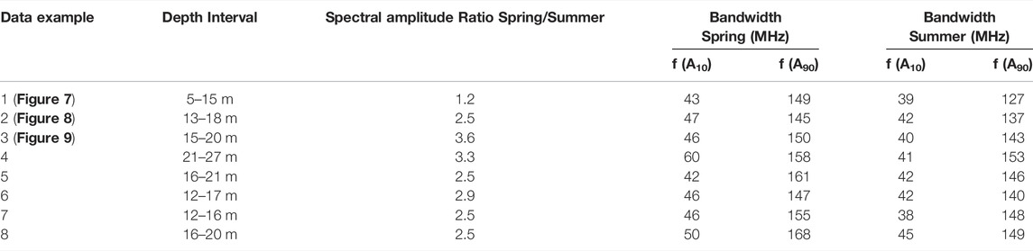
TABLE 1. Evaluation of amplitude spectra: amplitude ratio of spring to summer data and bandwidth (defined by 10th percentile A10 and 90th percentile A90). Depth interval is estimated for the time window of spring data and assuming v = 0.17 m/ns.
However, our observations may be partly related to our assumptions during data processing. For a more fair approach in terms of data interpretation, we calculate our spectral attributes on migrated data, incorporating a velocity model of the subsurface. For summer data our assumptions are likely to diverge stronger from the in situ GPR velocities (e.g., due to small-scale wetness heterogeneities in the active layer), leading to a weaker focusing of diffracted energy and a smoother appearance of reflections.
Several loss mechanisms affect an electromagnetic wave during propagation. These comprise spherical spreading, geometrical loss due to refraction, and intrinsic attenuation.
The loss due to spherical divergence results from the enlarging spherical surface of the electromagnetic pulse as the electromagnetic wave propagates concentrically away from the transmitter. Once emitted, the electromagnetic energy per surface element decreases with 1/t2 assuming a constant wavelength (i.e., constant propagation velocity).
Focusing effects at refraction interfaces result in geometrical loss (Bogorodsky et al., 1985). Here, due to the transition in another medium, the electromagnetic wavelength is altered resulting in an abrupt increase in electromagnetic energy per surface element (focusing effect for v2 < v1, i.e., if the velocity of the underlying layer is smaller) or an energy decrease (defocusing for v2 > v1). We calculate the radius of the first Fresnel Zone along an exemplary ray path and estimate a geometrical loss of −7 dB in summer with respect to spring at the lower boundary of the active layer.
Another signal loss mechanism we expect to differ in spring and summer is the intrinsic attenuation due to relaxation mechanism and electrical conduction. The intrinsic attenuation
with the electrical conductivity
We estimate the intrinsic attenuation for a thawed active layer using an electrical resistivity of
Thus, we relate our observed increase in energy loss from spring to summer dominantly to the strong electric contrast in summer and only to a minor part to the increase in electrical conductivity.
2D Finite-Difference Time-Domain Modelling
In the following, we use finite-difference time-domain (FDTD) modelling (Warren et al., 2016) to verify our observations in terms of synthetic 2D GPR data for our two scenarios. We rely our model on the borehole-based L14-02 ice content data (Schwamborn and Wetterich, 2016) shown in Figure 10A; i.e., a sediment core that was drilled during the spring survey in 2014 (for borehole location see Figures 1, 3). Taking into account typical bulk density values for Yedoma Ice Complex deposits (Strauss et al., 2013) and a two-phase CRIM model (Birchak et al., 1974), we calculate volumetric ice contents and the corresponding 1D GPR velocity function. We duplicate our 1D velocity function laterally and multiply the resulting 2D velocity field with a 2D noise model exhibiting small-scale heterogeneities (Figure 10B) to obtain our final 2D GPR velocity function. Figure 10C shows a vertical profile through our resulting velocity model, with the calculated velocity profile in black and the resulting velocity range for each depth in red.
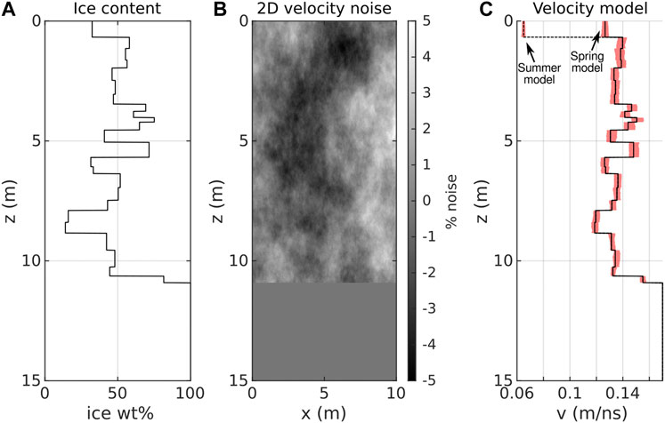
FIGURE 10. Construction of a heterogeneous 2D GPR velocity field for FDTD modeling. (A) gravimetric ice content of L14-02 (Schwamborn and Wetterich, 2016), (B) 2D stochastic noise field, (C) black: corresponding 1D GPR velocity model (black line) following a 2-phase CRIM model (Birchak et al., 1974) and the velocity range (red area) resulting from superposition with our 2D noise field.
Figure 11 shows our 2D FDTD modeling results for both the spring and the summer scenarios using source wavelets with center frequencies of 50, 100, and 200 MHz, respectively. All data are calculated for an antenna offset of 1 m. We applied an t2 amplitude scaling to correct for spherical divergence. For our synthetic spring scenario, the active layer is only resolved in the 200 MHz data. In 50 MHz and 100 MHz data the reflection of the lower active layer base is not visible due to the larger wavelength and antenna crosstalk. In contrast, the active layer bottom is detected at 100 MHz in the summer scenario due to the lower active layer GPR velocity. At ∼4.5–5.25 m depth, our velocity model exhibits a sequence of high velocity layers with thicknesses below 0.25 m. The sequence is resolved in the spring and the summer scenario at 100 and 200 MHz (with a different degree of detail), and integrated to a single reflector in our 50 MHz data due to the larger wavelength. A layer with lower GPR velocity at a depth of ∼8.5 m is resolved in both spring and summer data at 100 and 200 MHz in terms of two-sided reflections. For the 50 MHz data, this layer is only resolved as a single reflector. The transition to a massive ground ice body at a depth of z ∼ 11 m is resolved with all frequencies.
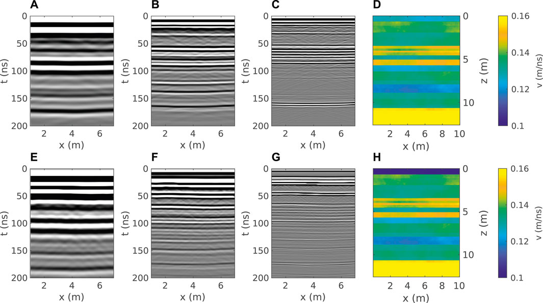
FIGURE 11. Finite-difference time-domain modeling results for our 2D velocity model for 50 MHz (A,E), 100 MHz (B,F), and 200 MHz (C,G) for spring and summer scenarios, respectively. The corresponding velocity models are shown in (D) and (H). Both models differ only in the uppermost 60 cm (active layer).
Although the number of resolved layers remains equal for each frequency, all layers resolved in our synthetic spring data are also resolved in our summer data. However, the spring data generally exhibit a higher contrast below the active layer, resulting in an easier interpretation and tracing of particular interfaces. For active layer imaging, an effective antenna mid-frequency of at least 100 MHz is recommended in summer and at least 200 MHz in spring.
Summary
For the first time, comparative 3D GPR observations have been undertaken at the same study area to point out advantages and disadvantages for deducing subsurface permafrost properties under completely frozen (springtime) and superficially thawed (summertime) conditions. Both datasets were collected using a nominal center frequency of 100 MHz. Summer GPR data differ from those obtained during spring due to the presence of an uppermost seasonally thawed active layer. This is seen in more complex waveform patterns at early times (i.e., t < 60 ns) in the summer data and results from interference between antenna crosstalk and reflected energy from the active layer base, while the spring data exhibit dominantly antenna crosstalk and less interference with reflected energy resulting in a less complex early time wavefield.
When comparing the surroundings of selected reflections recorded in summer and spring at different depths, the spring data show a higher dynamic range in amplitudes and a higher vertical resolution, resulting in a generally sharper image of subsurface structures, and the denoted reflectors appear more distinct. In contrast, the summer images provide a lower dynamic range and lower vertical resolution resulting in a smoother image of subsurface structures. This might ease reflector tracing and picking, but hinders a detailed imaging and interpretation as using the spring data.
Spectra of both data sets normalized to their respective total energy provide a consistent picture and differ much less than those of specific spring and summer reflection details. However, the spectra of our migrated summer data only contain around 40% of the energy compared to the spring data and also show a mean frequency downshift and bandwidth narrowing. We relate our observations dominantly to the strong increase in permittivity contrast at the active layer base in summer, but also to the increased superficial heterogeneity, causing our velocity model to deviate more likely from the actual in situ velocities. Although we show dominantly 2D data, a 3D survey setup is very important to ensure a successful migration by taking off-profile diffracted energy into account.
Due to topographic dynamics from season to season, we point out that combining datasets of different years will be challenging. Furthermore, a joint processing of data acquired at different seasons is not recommended. When interested in a larger picture of general reflectors of distinct (cryostratigraphic) units, which shall be traced in 3D, we recommend to perform the survey in summer to benefit from the smoother data. If active layer imaging is of major interest, we suggest an effective antenna mid-frequency of at least 100 MHz in summer and at least 200 MHz in spring, based on our modeling result. If detailed structural information is relevant and the object of interest is at the edge of resolution capabilities, we recommend performing the survey in spring. Thus, it is ensured to get the best performance with the drawback of more complex interpretation and higher surveying effort (e.g., related to lower battery performance and harsher conditions for field work).
Data Availability Statement
The datasets presented in this study can be found in online repositories. The names of the repository/repositories and accession number(s) can be found below: The datasets analyzed for this study can be found in the PANGAEA data repository (https://doi.org/10.1594/PANGAEA.868978, https://doi.org/10.1594/PANGAEA.859798).
Author Contributions
SS and JT contributed to conception of the study and acquired the survey data. SW, GS, and LS conducted sediment sampling and analysis. SS wrote the first draft of the manuscript. SW wrote the section survey site. All authors contributed to manuscript revision, read, and approved the submitted manuscript.
Funding
We gratefully acknowledge the German Federal Ministry of Education and Research (BMBF) for funding this study as part of the CARBOPERM project (03G0836B, 03G0836J).
Conflict of Interest
The authors declare that the research was conducted in the absence of any commercial or financial relationships that could be construed as a potential conflict of interest.
The handling editor and the reviewer AV are currently organizing a Research Topic with the author LS.
Publisher’s Note
All claims expressed in this article are solely those of the authors and do not necessarily represent those of their affiliated organizations, or those of the publisher, the editors, and the reviewers. Any product that may be evaluated in this article, or claim that may be made by its manufacturer, is not guaranteed or endorsed by the publisher.
Acknowledgments
We thank M. Dubnitzki, W. Schneider, and V. Zykov for technical and logistical support. Furthermore, we thank N. Allroggen for his support in acquiring the spring data set and two reviewers for their valuable comments on the manuscript.
Supplementary Material
The Supplementary Material for this article can be found online at: https://www.frontiersin.org/articles/10.3389/feart.2022.741524/full#supplementary-material
References
Allroggen, N., Tronicke, J., Delock, M., and Böniger, U. (2015). Topographic Migration of 2D and 3D Ground‐penetrating Radar Data Considering Variable Velocities. Near Surf. Geophys. 13, 253–259. doi:10.3997/1873-0604.2014037
AMAP (2021). Arctic Climate Change Update 2021: Key Trends and Impacts. Summary for Policy-makersArctic Monitoring and Assessment Programme (AMAP). Tromsø, Norway, 16.
Andreev, A. A., Grosse, G., Schirrmeister, L., Kuznetsova, T. V., Kuzmina, S. A., Bobrov, A. A., et al. (2009). Weichselian and Holocene Palaeoenvironmental History of the Bol'shoy Lyakhovsky Island, New Siberian Archipelago, Arctic Siberia. Boreas 38, 72–110. doi:10.1111/j.1502-3885.2008.00039.x
Andreev, A. A., Schirrmeister, L., Tarasov, P. E., Ganopolski, A., Brovkin, V., Siegert, C., et al. (2011). Vegetation and Climate History in the Laptev Sea Region (Arctic Siberia) during Late Quaternary Inferred from Pollen Records. Quat. Sci. Rev. 30, 2182–2199. doi:10.1016/j.quascirev.2010.12.026
Andreev, A., Grosse, G., Schirrmeister, L., Kuzmina, S., Novenko, E., Bobrov, A., et al. (2004). Late Saalian and Eemian Palaeoenvironmental History of the Bol'shoy Lyakhovsky Island (Laptev Sea Region, Arctic Siberia). Boreas 33, 319–348. doi:10.1111/j.1502-3885.2004.tb01244.x
Arkhangelov, A. A., Mikhalev, D. V., and Nikolaev, V. I. (1996). “About Early Epochs of Permafrost Formation in Northern Yakutia and Age of Ancient Relicts of Underground Glaciation,” in Razvitie Oblasti Mnnogoletnei Merzloty I Periglyatsial’noi Zony Severnoi Evrazii I Usloviya Rasseleniya Drev- Nego Cheloveka. Editors A. A. Velichko, A. A. Arkhangelov, O. K. Borisova, Y. N. Gribchenko, A. N. Drenova, E. M. Zeliksonet al. (Moscow: Institute of Geography), 102–109. (in Russian).
Birchak, J. R., Gardner, C. G., Hipp, J. E., and Victor, J. M. (1974). High Dielectric Constant Microwave Probes for Sensing Soil Moisture. Proc. IEEE 62, 93–98. doi:10.1109/PROC.1974.9388
Biskaborn, B. K., Smith, S. L., Noetzli, J., Matthes, H., Vieira, G., Streletskiy, D. A., et al. (2019). Permafrost Is Warming at a Global Scale. Nat. Commun. 10, 1–264. doi:10.1038/s41467-018-08240-4
Bogorodsky, V. V., Bentley, C. R., and Gudmansen, P. E. (1985). Radioglaciology, Glaciology and Quaternary Geology. Dodrecht, Holland: D. Reidel Publishing Company.
Boniger, U., and Tronicke, J. (2010). On the Potential of Kinematic GPR Surveying Using a Self-Tracking Total Station: Evaluating System Crosstalk and Latency. IEEE Trans. Geosci. Remote Sensing 48, 3792–3798. doi:10.1109/TGRS.2010.2048332
Brosten, T. R., Bradford, J. H., McNamara, J. P., Gooseff, M. N., Zarnetske, J. P., Bowden, W. B., et al. (2009). Estimating 3D Variation in Active-Layer Thickness beneath Arctic Streams Using Ground-Penetrating Radar. J. Hydrol. 373, 479–486. doi:10.1016/j.jhydrol.2009.05.011
Bunge, A. A. (1887). “Bericht ueber den ferneren Gang der Expedition. Reise nach den Neusibirischen Inseln. Aufenthalt auf der Grossen Ljachof-Insel,” in Expedition zu den Neusibirischen Inseln und dem Jana-Lande (1885). Beitraege zur Kenntnis des russischen Reiches und der angrenzenden Laender. Editors L. V. Schrenk, and C. J. Maximovicz, III, 231–284. (in German).
Campbell, S., Affleck, R. T., and Sinclair, S. (2018). Ground-penetrating Radar Studies of Permafrost, Periglacial, and Near-Surface Geology at McMurdo Station, Antarctica. Cold Regions Sci. Tech. 148, 38–49. doi:10.1016/j.coldregions.2017.12.008
GISTEMP Team (2021). GISS Surface Temperature Analysis (GISTEMP), Version 4. NASA Goddard Institute for Space Studies. Dataset. Available at: data.giss.nasa.gov/gistemp/(accessed 05 01, 2021).
Grigoreva, S. D., Kiniabaeva, E. R., Kuznetsova, M. R., Popov, S. V., and Kashkevich, M. P. (2020). Examples of Application of GPR for Ensuring Safety of Infrastructure Objects at the Area of the Russian Antarctic Station Progress (East Antarctica). Proc. EAGE Eng. Mining Geophys. 2020, 1–11. doi:10.3997/2214-4609.202051010
Koven, C. D., Schuur, E. A. G., Schädel, C., Bohn, T. J., Burke, E. J., Chen, G., et al. (2015). A Simplified, Data-Constrained Approach to Estimate the Permafrost Carbon-Climate Feedback. Phil. Trans. R. Soc. A. 373, 205420140423. doi:10.1098/rsta.2014.0423
Kunitsky, V. V. (1998). “Ice Complex and Cryoplanation Terraces of Bol’shoy Lyakhovsky Island,” in Problems of Geocryology. Collected Papers. Editors R. M. Kamensky, V. V. Kunitsky, B. A. Olovin, and V. V. Shepelev (Yakutsk: RAS, Permafrost Institute), 60–72. (in Russian).
Meredith, M., Sommerkorn, M., Cassotta, S., Derksen, C., Ekaykin, A., Hollowed, A., et al. (2019). “Polar Regions,” in IPCC Special Report on the Ocean and Cryosphere in a Changing Climate. Editors H. O. Pörtner, D. C. Roberts, V. Masson-Delmotte, P. Zhai, M. Tignor, E. Poloczanskaet al. In press. accessed on 2021-05-22. https://www.ipcc.ch/srocc/chapter/chapter-3-2/.
Nagaoka, D. (1994). “Properties of Ice Complex Deposits in Eastern Siberia,” in Proceedings of the 2nd Symposium on the Joint Siberian Permafrost Studies between Japan and Russia in 1993, Tsukuba, Japan, 14–18.
Nagaoka, D., Saijo, K., and Fukuda, M. (1995). “Sedimental Environment of the Edoma in High Arctic Eastern Siberia,” in Proceedings of the 3rd Symposium on the Joint Siberian Permafrost Studies between Japan and Russia, Tsukuba, Japan. Editors K. Takahashi, A. Osawa, and Y. Kanazawa (Hokkaido University), 8–13.
Oezen, L. D., and Geyh, M. A. (2002). 230Th/U Dating of Frozen Peat, Bol'shoy Lyakhovsky Island (Northern Siberia). Quat. Res. 57, 253–258. doi:10.1006/qres.2001.2306
Romanovskii, N. N. (1958a). New Data about Quaternary Deposits Structure on the Bol’shoy Lyakhovsky Island (Novosibirskie Islands). Nauchnye Doklady Vysshei Shkoly. Seriya Geologo-geograficheskaya 2, 243–248. (in Russian).
Romanovskii, N. N. (1958b). “Paleogeographic Conditions of Formation of the Quaternary Deposits on Bol’shoy Lyakhovsky Island (Novosibirskie Islands),” in Voprosy Fizicheskoi Geografii Polyarnykh Stran. Vypysk I. Editor V. G. Bogorov (Moscow: Moscow State University), 80–88. (in Russian).
Romanovskii, N. N. (1958c). Permafrost Structures in Quaternary Deposits. Nauchnye Doklady Vysshei Shkoly. Seriya Geologo-geograficheskaya 3, 185–189. (in Russian).
Schennen, S., Allroggen, N., and Tronicke, J. (2015). “Near Surface Geophysics,” Russian-German Cooperation CARBOPERM: Field Campaigns to Bol’shoy Lyakhovsky Island in 2014. Editors G. Schwamborn, and S. Wetterich Reports on Polar and marine Research 686, 48–63. doi:10.2312/BzPM_0686_2015
Schennen, S., Tronicke, J., Wetterich, S., Allroggen, N., Schwamborn, G., and Schirrmeister, L. (2016). 3D Ground-Penetrating Radar Imaging of Ice Complex Deposits in Northern East Siberia. Geophysics 81 (1), WA195–WA202. doi:10.1190/geo2015-0129.1
Schirrmeister, L., Oezen, D., and Geyh, M. A. (2002). 230Th/U Dating of Frozen Peat, Bol’shoy Lyakhovsky Island (Northern Siberia). Quaternary Research 57, 253–258. doi:10.1006/qres.2001.2306
Schmid, L., Heilig, A., Mitterer, C., Schweizer, J., Maurer, H., Okorn, R., et al. (2014). Continuous Snowpack Monitoring Using Upward-Looking Ground-Penetrating Radar Technology. J. Glaciol. 60, 509–525. doi:10.3189/2014JoG13J084
Schwamborn, G. J., Dix, J. K., Bull, J. M., and Rachold, V. (2002). High-resolution Seismic and Ground Penetrating Radar-Geophysical Profiling of a Thermokarst lake in the Western Lena Delta, Northern Siberia. Permafrost Periglac. Process. 13 (4), 259–269. doi:10.1002/ppp.430
Schwamborn, G., Heinzel, J., and Schirrmeister, L. (2008a). Internal Characteristics of Ice-Marginal Sediments Deduced from Georadar Profiling and Sediment Properties (Brøgger Peninsula, Svalbard). Geomorphology 95, 74–83. doi:10.1016/j.geomorph.2006.07.032
Schwamborn, G., Wagner, D., and Hubberten, H.-W. (2008b). The Use of GPR to Detect Active Layers in Young Periglacial Terrain of Livingston Island, Maritime Antarctica. Near Surf. Geophys. 6, 331–336. doi:10.3997/1873-0604.2008008
Schwamborn, G., and Wetterich, S. (2016). Geochemistry and Physical Properties of Permafrost Core L14-02. PANGAEA. doi:10.1594/PANGAEA.868978
Strauss, J., Schirrmeister, L., Grosse, G., Fortier, D., Hugelius, G., Knoblauch, C., et al. (2017). Deep Yedoma Permafrost: A Synthesis of Depositional Characteristics and Carbon Vulnerability. Earth-Science Rev. 172, 75–86. doi:10.1016/j.earscirev.2017.07.007
Strauss, J., Schirrmeister, L., Grosse, G., Wetterich, S., Ulrich, M., Herzschuh, U., et al. (2013). The Deep Permafrost Carbon Pool of the Yedoma Region in Siberia and Alaska. Geophys. Res. Lett. 40, 6165–6170. doi:10.1002/2013gl058088
Tumskoy, V. E. (2012). Osobennosti Kriolitogeneza Otlozhenii Severnoi Yakutii V Srednem Neopleistotsene-Golotsene (Peculiarities of Cryolithogenesis in Northern Yakutia from the Middle Neopleistocene to the Holocene). Kriosfera Zemli 16, 12–21. (in Russian).
von Toll, E. V. (1897). Iskopaemye Ledniki Novo-Sibirskikh Ostrovov, Ikh Otnoshenie K Trupam Mamontov I K Lednikovomu Periodu (Ancient Glaciers of New Siberian Islands, Their Relation to mammoth Corpses and the Glacial Period). Zapiski Imperatorskogo Russkogo Geograficheskogo Obshestvapo Obshei Geografii (Notes of the Russian Imperial Geographical Society) 32, 1–137.
Warren, C., Giannopoulos, A., and Giannakis, I. (2016). gprMax: Open Source Software to Simulate Electromagnetic Wave Propagation for Ground Penetrating Radar. Comp. Phys. Commun. 209, 163–170. doi:10.1016/j.cpc.2016.08.020
Wetterich, S., Meyer, H., Fritz, M., Mollenhauer, G., Rethemeyer, J., Kizyakov, A., et al. (2021). Northeast Siberian Permafrost Ice‐Wedge Stable Isotopes Depict Pronounced Last Glacial Maximum Winter Cooling. Geophys. Res. Lett. 48, e2020GL092087. doi:10.1029/2020GL092087
Wetterich, S., Rudaya, N., Kuznetsov, V., Maksimov, F., Opel, T., Meyer, H., et al. (2019). Ice Complex Formation on Bol'shoy Lyakhovsky Island (New Siberian Archipelago, East Siberian Arctic) since about 200 ka. Quat. Res. 92 (2), 530–548. doi:10.1017/qua.2019.6
Wetterich, S., Rudaya, N., Tumskoy, V., Andreev, A. A., Opel, T., Schirrmeister, L., et al. (2011). Last Glacial Maximum Records in Permafrost of the East Siberian Arctic. Quat. Sci. Rev. 30, 3139–3151. doi:10.1016/j.quascirev.2011.07.020
Wetterich, S., Schirrmeister, L., Andreev, A. A., Pudenz, M., Plessen, B., Meyer, H., et al. (2009). Eemian and Late Glacial/Holocene Palaeoenvironmental Records from Permafrost Sequences at the Dmitry Laptev Strait (NE Siberia, Russia). Palaeogeogr. Palaeoclimatol. Palaeoecol. 279, 73–95. doi:10.1016/j.palaeo.2009.05.002
Wetterich, S., Tumskoy, V., Rudaya, N., Andreev, A. A., Opel, T., Meyer, H., et al. (2014). Ice Complex Formation in Arctic East Siberia during the MIS3 Interstadial. Quat. Sci. Rev. 84, 39–55. doi:10.1016/j.quascirev.2013.11.009
Wetterich, S., Tumskoy, V., Rudaya, N., Kuznetsov, V., Maksimov, F., Opel, T., et al. (2016). Ice Complex Permafrost of MIS5 Age in the Dmitry Laptev Strait Coastal Region (East Siberian Arctic). Quat. Sci. Rev. 147, 298–311. doi:10.1016/j.quascirev.2015.11.016
Yoshikawa, K., Leuschen, C., Ikeda, A., Harada, K., Gogineni, P., Hoekstra, P., et al. (2006). Comparison of Geophysical Investigations for Detection of Massive Ground Ice (Pingo Ice). J. Geophys. Res. 111, E06S19. doi:10.1029/2005JE002573
Zimmermann, H., Raschke, E., Epp, L., Stoof-Leichsenring, K., Schirrmeister, L., Schwamborn, G., et al. (2017). The History of Tree and Shrub Taxa on Bol'shoy Lyakhovsky Island (New Siberian Archipelago) since the Last Interglacial Uncovered by Sedimentary Ancient DNA and Pollen Data. Genes 8, 273E273. doi:10.3390/genes8100273
Keywords: GPR, seasonal effects, resolution, yedoma, permafrost
Citation: Schennen S, Wetterich S, Schirrmeister L, Schwamborn G and Tronicke J (2022) Seasonal Impact on 3D GPR Performance for Surveying Yedoma Ice Complex Deposits. Front. Earth Sci. 10:741524. doi: 10.3389/feart.2022.741524
Received: 14 July 2021; Accepted: 07 March 2022;
Published: 19 April 2022.
Edited by:
Go Iwahana, University of Alaska Fairbanks, United StatesReviewed by:
Tatsuya Watanabe, Kitami Institute of Technology, JapanAlexandra Veremeeva, Institute of Physical-Chemical and Biological Problems in Soil Science (RAS), Russia
Copyright © 2022 Schennen, Wetterich, Schirrmeister, Schwamborn and Tronicke. This is an open-access article distributed under the terms of the Creative Commons Attribution License (CC BY). The use, distribution or reproduction in other forums is permitted, provided the original author(s) and the copyright owner(s) are credited and that the original publication in this journal is cited, in accordance with accepted academic practice. No use, distribution or reproduction is permitted which does not comply with these terms.
*Correspondence: Stephan Schennen, c3RlcGhhbi5zY2hlbm5lbkBsZWlibml6LWxpYWcuZGU=
†Present Address: Stephan Schennen, Leibniz Institute for Applied Geophysics, Hanover, GermanySebastian Wetterich, Heisenberg Chair of Physical Geography with Focus on Paleoenvironmental Research, Institute of Geography, Dresden, Technische Universität Dresden, GermanyGeorg Schwamborn, Eurasian Institute of Earth Sciences, Istanbul Technical University, Istanbul, Turkey