Thickness Variation Characteristics of Tidal Rhythmites—An Example From the Pinghu Formation, Xihu Sag, East China Sea Shelf Basin

The Pinghu Formation of the Xihu Sag in the East China Sea shelf basin is influenced by tidal processes, but few studies have focused on its tidal rhythmites. Through detailed observation and description of cores, this article studies the periodicity of the tidal rhythmites of well A-11 by using the grayscale measurement of digital images based on spectral analysis and wavelet transform. According to the statistical data series of millimeter lamination thickness, the sandy lamina thickness, the argillaceous lamina thickness, and the couplet thickness were quantitatively compared and analyzed, to support the interpretation of the main controlling factors of different thickness cycles. The periodicity of sandy laminae, argillaceous laminae, and couplet thickness have distinct differences, which are interpreted to be due to differences in the nature and magnitude of tidal current cycles at the time of deposition. The high-frequency signal represents event deposition, the middle-frequency signal represents tidal current deposition, and the low-frequency signal highlights changes in sedimentary facies. Therefore, the change in the couplet thickness is controlled by event deposition, tidal current deposition, and change of the depositional environment. Our approach to the study of thickness variations in tidal rhythmites supports the reconstruction of the tidal sedimentary environment in the paleostratigraphic sequence.

Introduction

Tidal depositional systems are the product of sedimentary environments dominated or influenced by the effects of tides. Sediments deposited under tidal hydrodynamics are distributed and organized into specific sedimentary facies, which preserve strong tidal constituents influencing a given coastal area (Wu, 1994; Wu, 1996; Gao et al., 2000; Zhou et al., 2002; Zhao et al., 2008). Tidal environments, whether deltaic or estuarine, are commonly classified as supratidal, intertidal, and subtidal (Zhao et al., 2008). The general term “tidalites” (Wu, 1994; Wu, 1996) refers to deposits with tidal signatures exhibited as rhythmites. The thickness and frequency of sandy laminae and argillaceous laminae in tidal rhythmites bedding record the tidal cycle and the magnitude of tidal energy. Through the study of tidal rhythmites, the tidal deposition process can be reconstructed, and the periodic characteristics of tidal deposition can be inferred. Tidal cycles have been studied at different scales in the deposition process (Tessier and Gigot, 1980; Visser, 1980; Yang and Nio, 1985; Williams, 1989; Kvale and Archer, 1990; Kvale et al., 1999; Li et al., 2000; Zhou et al., 2002; Bádenas et al., 2003; Hovikoski et al., 2005; Frouin et al., 2006; Longhitano et al., 2012; Bhattacharya et al., 2019) by analyzing the changes of both the thickness and number of couplets in rhythmites. Tidal rhythmites have become an important indicator for high-resolution paleoenvironmental reconstructions.

The East China Sea shelf basin is an important petroliferous basin in China, and the Eocene Pinghu Formation is one of the main target strata for oil and gas exploration in Xihu Sag. Before and after the deposition of the Pinghu Formation, the Yandang, Oujiang, and Yuquan tectonic movements occurred, resulting in a complicated paleogeomorphology and major changes in sedimentary environments. Previous scholars disagree on the sedimentary model for the Pinghu Formation. Jiang et al. (2011) used micropaleontological fossils to propose that the upper Pinghu Formation and Huagang Formation were the continental deposits. Yang et al. (2013) proposed that the sandbody morphology and sedimentary sequence of E₂p in the Pinghu slope zone support interpretation of a braided delta in a shallow water environment. Liu et al. (2009) proposed that an alluvial fan, a nearshore subaqueous fan, and a turbidite fan developed in the early and middle stages of the Pinghu Formation, and a braided river delta and fan delta developed in the middle and late stages of the Pinghu Formation, and tidal flat deposits mainly developed in the late stages of the Pinghu Formation. Recently, there has been a convergence in interpretation on the role of tidal processes and deposits. Zhao Lina et al. (Zhao, 2007) proposed that the Pinghu Formation in the Pinghu structural zone of the Xihu Sag could be divided into two main sedimentary facies types: the tidal sedimentary facies and tidal delta sedimentary facies. Wu Jiapeng (Wu et al., 2017) divided the lithofacies of the Pinghu Formation into three types: the conglomerate facies, sandstone facies, and fine-grained lithofacies and interpreted delta facies, tidal flat facies, and restricted marine facies influenced by tidal action. Yu et al. (2017) interpreted that the Pinghu Formation is a tidal fluvial delta sedimentary system and a tidal flat sedimentary system.

The general understanding of the tidal sedimentary environments of the Pinghu Formation is relatively mature, but detailed analysis remains rare. Based on the detailed observation and description of the cores of well A-11 of the Pinghu Formation in the Xihu Sag, East China Sea Shelf Basin, a large number of tidal sedimentary structures have been identified. Software was used to analyze the periodicity of the variation of the couplet thicknesses, using measurements of the sandy laminae and the argillaceous laminae thicknesses, and to discuss the geological mechanism of the periodic variation of the three so as to provide a reference for the reconstruction of the regional paleoenvironment.

Geological Setting

The Xihu Sag is the largest oil-gas structural belt in the East China Sea shelf basin. Its eastern boundary is the Diaoyu Island fold belt, and it is adjacent to the Diaobei Sag and the Fujiang Sag in the south and north, respectively. In the west, from north to south, it is connected with five tectonic units: the Hubijiao Uplift, Changjiang Sag, Haijiao Uplift, Qiantang Sag, and Yushan Uplift (Figure 1A), with a north-south length of about 440 km, an east-west width of about 110 km, and a total area of about 51,800 km² (Abbas et al., 2018; Zhao et al., 2018; Chen et al., 2020; Cheng et al., 2020; Jiang et al., 2020). The Xihu Sag of the Cenozoic strata intersected from the bottom to top of the Eocene Oujiang Formation, Wenzhou Formation, and Pinghu Formation, Huagang Formation of Oligocene, Longjing Formation, Yuquan Formation and Liulang Formation of Miocene, Santan Formation of Pliocene, and Donghai Formation of Quaternary (Figure 1B). The Pinghu Formation and Huagang Formation are the main oil and gas exploration target strata in this area. Well A-11, located in the western slope belt of the sag, was drilled into the Eocene Pinghu Formation at a depth of 3,856.6–3,865.89 m in the core section. The tidal sedimentary structures of the cores in this section are well developed, and the sedimentary structures include interbedded sandy and argillaceous, double clay layers and couplets (Figure 2).

FIGURE 1

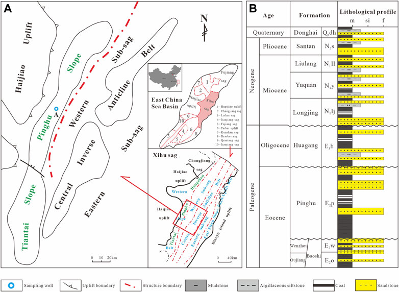
FIGURE 1. Geological maps showing: (A) Tectonic characteristics of the Xihu Sag, East China Sea shelf basin; (B) Comprehensive stratigraphic column of the Xihu Sag, East China Sea shelf basin.

FIGURE 2

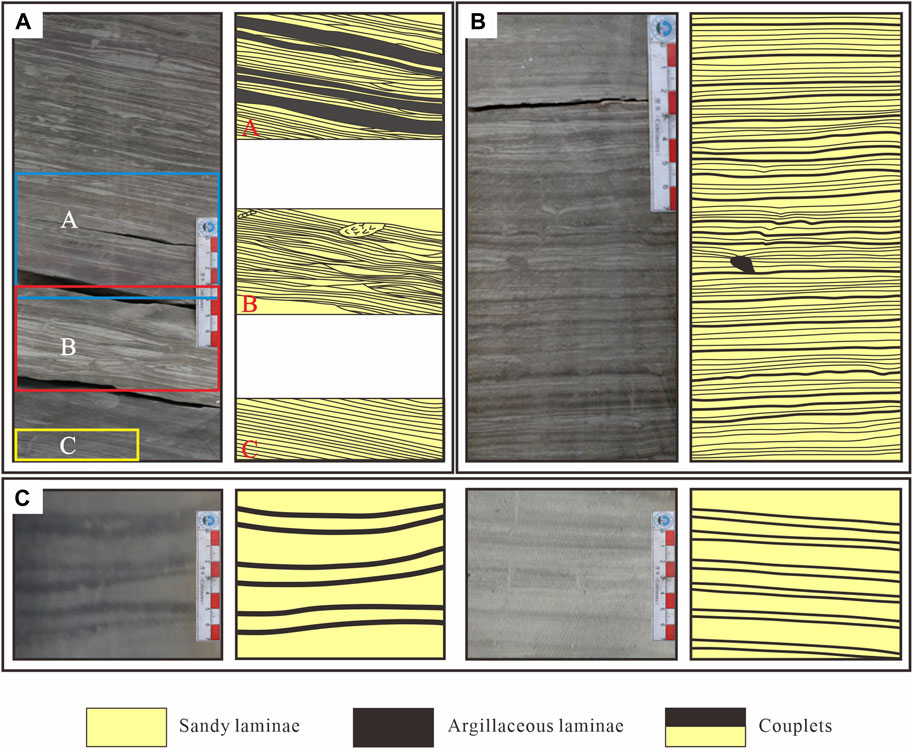
FIGURE 2. Typical sedimentary characteristics of well A-11 of the Pinghu Formation in the Xihu Sag, East China Sea shelf basin. (A) interbedded sandy and argillaceous, A-flaser bedding, B-lenticular bedding, and C-interbedded sandy and argillaceous; (B) couplet; (C) double clay layer.

In this study, the core was observed and described in detail (1:5 vertical resolution), and the sedimentary structure, lithologic characteristics, lithofacies, and their association relations were analyzed. Combined with the analysis of laboratory data, it was considered that the core section represented tidal flat deposits. We selected five sets of sandy-argillaceous beds with depths of 3,856.60–3,858.50 m, 3,858.50–3,860.20 m, 3,860.20–3,860.45 m, 3,862.25–3,863.45 m, and 3,863.45–3,865.89 m, in which the first section is interpreted as a sand flat deposit, the second section and fifth section are interpreted as a mixed flat deposit, the third section is interpreted as a mud flat deposit, and the fourth section is interpreted as a tidal channel deposit (Figure 3).

FIGURE 3

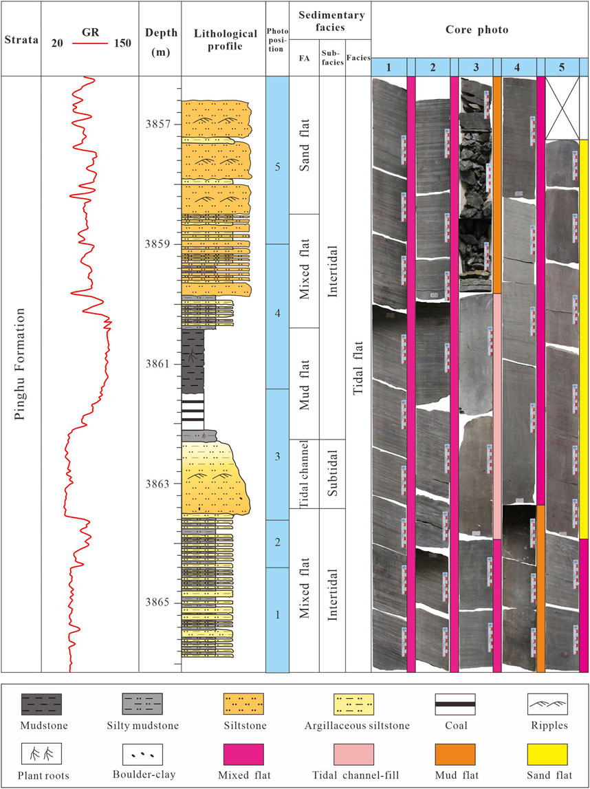
FIGURE 3. Lithologic column of well A-11 of the Pinghu Formation in the Xihu Sag, East China Sea shelf basin. Note that the Pinghu Formation consists of tidal flat units consisting of interbedded sandstone and mudstone. GR is the natural gamma ray log. FA is lithofacies associations.

Data Sets and Methodology

Data Sets

All data were collected from core images, and fine core observations were performed in the core bank of CNOOC Shanghai branch. The analysis of the lamina’s thickness in the core section of well A-11 in the Pinghu Formation (3,856.6∼3,865.89 m), which included the measurement of the thickness of the layer, frequency spectrum analysis, and wavelet analysis, was conducted in the Yangtze University laboratory.

Methodology

The measurement of the thickness of sandy and argillaceous laminae is the basis of studying tidal rhythmites. In this study, core images with depth scales were first adjusted to the extent that the minimum couplet could be clearly observed. However, due to the limitation of measurement accuracy, it is difficult to measure the thin argillaceous laminae mixed in the thicker sandy laminae, or conversely to measure the thin sandy laminae mixed in the thicker argillaceous laminae. Therefore, our statistical couplet thicknesses include a thicker sandy lamina thickness and the adjacent thicker argillaceous lamina thickness. In addition, some of the finer laminae are not continuous across the core. The route of the survey line should be selected on the profile line with clear laminae and an obvious growth zone. We measured as many laminae as possible. Through multiple tests on different paths in the core image, it was proved that the laminae identified in the midline path were the most complete. We used MATLAB software to automate identification of the sandy and argillaceous laminae thicknesses from the images. Each of the sandy and argillaceous laminae was numbered, and the laminae thickness of the five sets of tidal rhythmites was calculated. The linewidth of image information acquisition was measured in PIX units (i.e., pixels), and an appropriate linewidth of the filter kernel was set. When the filter kernel is set too small, the resolution is higher, but it is easily interfered by local factors in the measurement path, such as 1pix (Figure 4); when the filter core is set too large, the influence of the background blot noise can be reduced, and the signal of high-resolution lamination is easily lost, such as 5pix, 7pix, 9pix, and 11pix (Figure 4) (Yi et al., 2010; Wu et al., 2012; Yi, 2012; Lopes et al., 2018). The filter core is generally set as an odd number, but the 1pix filter kernel does not have the filter denoising function (Figure 4). Different filtering mechanisms were used to carry out multiple acquisitions in the same path. Therefore, from the comprehensive consideration of the denoising effect and lamina recognition clarity, the best acquisition effect was determined, when the filter core was set at 3pix (Figure 4). Based on the color difference of different lithologies, the core image is converted into a grayscale image, and binarization image denoising is carried out to obtain the binarization result of a single point on the midline. The continuous pixel length of the binarization result is counted, and the result is converted into the actual length. The continuous pixel length of each binarization result represents the lithology and thickness of the sandy and argillaceous laminae; thus, the actual thickness corresponding to each lamina can be obtained. In this study, a total of 1,530 lamina thicknesses and 765 couplets of sandy and argillaceous layers were counted (Table 1).

FIGURE 4

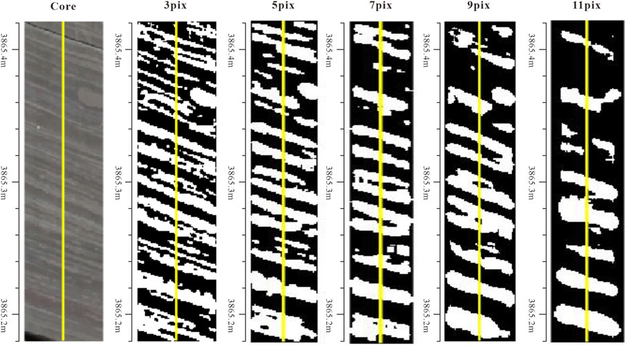
FIGURE 4. Comparison of the results of core images collected under different filter cores (3,865.28 m∼3,865.41 m).

TABLE 1

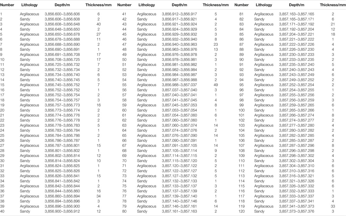
TABLE 1. Statistics of sandy and argillaceous lamina thicknesses of well A-11 in the Pinghu formation.

To verify the feasibility of this method, the clearest part of the sample was taken for manual calculation rather than the whole sample. Manual counting requires the naked eye combined with a mirror to carefully distinguish the lamina, and then, the lamina thickness was calculated through the scale. Therefore, in the case of an unclear lamina, the result of manual calculation is not accurate enough, and its comparative analysis has little significance. Figure 5 shows a total of 46 laminae calculated by software using the above method, with the maximum thickness of 10 mm. The number of manual counting laminae is 44; the maximum thickness of laminae is 10 mm. There are only two laminae of the difference between the two. Therefore, the number of laminae calculated by the two methods is almost consistent. In addition, from the position of lamina thickness peaks, there is little difference between the two, almost at the same position. The results of manual counting and software calculation can correspond well in both the laminar number and laminar thickness, which proves the feasibility of this method.

FIGURE 5

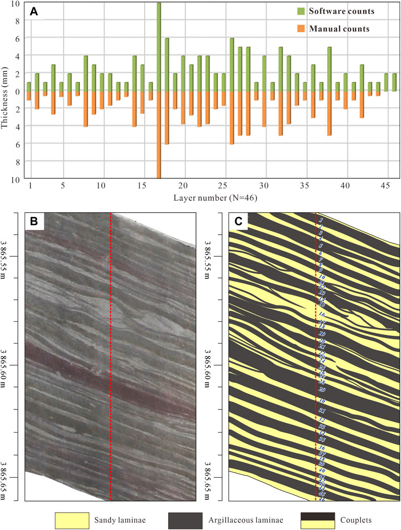
FIGURE 5. Laminae were compared by manual counts and software count results. (A) is a comparison of the two methods. (B) is a photo of the measured core, and (C) is a sketch of its core.

The spectrum analysis is carried out after interpolation, de-extrema and de-trend preprocessing for lamina data. Spectrum analysis is the most commonly used statistical analysis method in the study of periodic phenomena. Its basic principle is to decompose the composite wave system into several simple harmonics with different amplitudes and phases through data transformation and then calculate the period value according to the main frequency of the wavelet (Zhao et al., 2009). First, the spectrum analysis program RedFit3.8 was used to calculate the fast Fourier transform (FFT) (Li et al., 2006; Santos et al., 2020; Fontana et al., 2021) for each lamina thickness data sequence under the background of red noise, and the characteristic period distribution of lamina thickness was explained. Second, on this basis, through AnalySeries 2.08 software of low pass filtering function to remove the high-frequency factor such as wave abnormalities, the coring grain layer thickness of lithofacies association cycle information was extracted, and analysis of the periodicity of the couplet, the sandy laminae, and the argillaceous lamina thickness was carried out. Third, wavelet analysis was used to eliminate the influence of the tidal current cycle from the variation of the thickness of sandy laminae and argillaceous laminae. Finally, the quantitative characterization of the current cycle and sedimentary facies of the change had an impact on the lamina thickness change, respectively. Wavelet analysis not only retains the advantages of the Fourier transform but also makes up for the deficiency that the Fourier transform cannot reflect signal characteristics in local time (space). Many scholars have introduced this method into a high-precision sequence unit division to amplify the information in logging signals and to identify sequence cycles of different levels (Zhu et al., 2010; Chen et al., 2018; He, 2020; Fontana et al., 2021). Through frequency division processing on the data on variation in the thickness of sandy laminae, argillaceous laminae, and couplets, the frequency division signal was extracted and compared with the sedimentary facies divided by core observations, and the corresponding relationship between the frequency signal and sedimentary facies was summarized.

Result

Variation Characteristics of the Lamina Thickness

The thickness of each sandy lamina, argillaceous lamina, and couplet, as well as the variation of the thickness of adjacent laminae, was obtained statistically (Table 2). It can be seen from the table that the thicknesses of couplets and laminae range dramatically, such as some adjacent laminae are quite different in thickness, although some in successions have a relatively consistent thickness. The thickness of the adjacent laminae is rather variable, which has affected the periodicity analysis. At first, the laminae’s thickness was numbered and arranged, and then, the interpolated preprocessing of the data was performed in order to enhance the trend of the data and facilitate the mining of periodic regularity (Figure 6).

TABLE 2

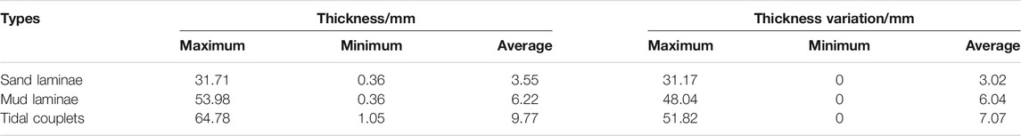
TABLE 2. Statistics of the tidal couplet thickness variation of well A-11 in the Pinghu formation.

FIGURE 6

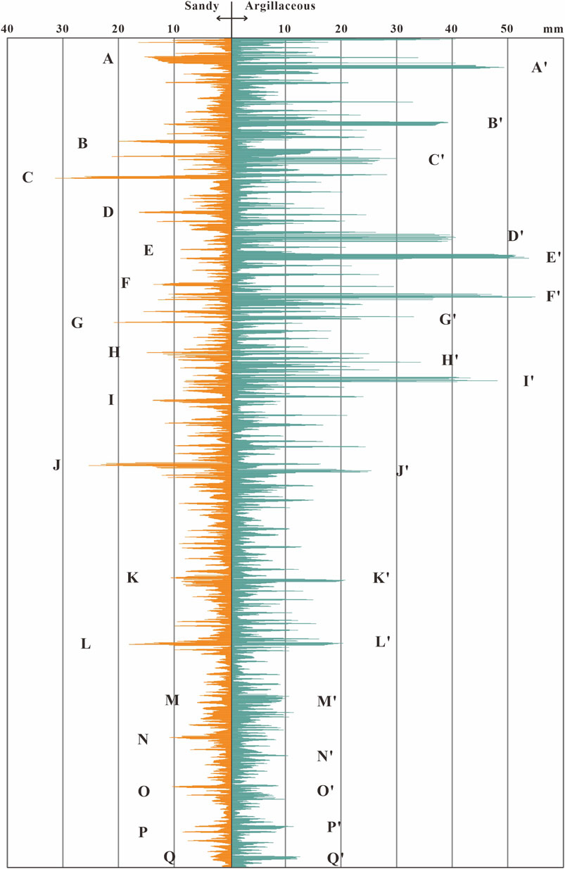
FIGURE 6. Statistical results of the sandy and argillaceous lamina thicknesses of well A-11 in the Pinghu Formation.

The thickness of sandy laminae has 17 cycles (No. A–No. Q) and that of the argillaceous laminae has 17 cycles (No. A′–No. Q′) (Figure 6). The periods of the cycles are different. From cycle D′–cycle I′, the thicknesses of argillaceous laminae are large, but the number of laminae is smaller than those of cycle D–cycle I. After comparing the variation of the thickness period of sandy and argillaceous laminae, it can be found that they are correlated but without the same trends. The sandy laminae and argillaceous laminae can both vary at the maximum, such as cycle E–cycle F and cycle E′–cycle F′, cycle J–cycle L and cycle J′–cycle L′, and cycle O–cycle Q and cycle O′–cycle Q′. Also, cycle A–cycle D and cycle A′–cycle D′, and cycle M–cycle N and cycle M′–cycle N′ do not reach the summit at the same lamina number, with the disparity of about 10 laminae. All the cycles are combined responses of the sedimentary dynamics and the environment of deposition.

Spectral Analysis

In order to accurately identify the period of the lamina thickness, spectral analysis was performed on the data. Generally, the higher the power value is, the stronger the signal of this period appears in the data series. According to the 99% confidence curve test of red noise, the couplet frequency points are 0.054, 0.104, and 0.120 (Figure 7A); the argillaceous lamina frequency points are 0.054, 0.104, and 0.120 (Figure 7B); the sandy lamina frequency points are 0.054, 0.091, 0.104, and 0.120 (Figure 7C). The reciprocal of the frequency value can obtain the corresponding period or cycle number (Li et al., 2006; Zhao et al., 2009; Santos et al., 2020). As can be seen from the spectrum figure (Figure 7), the spectral peaks of the strongest signals of the lamina thickness, argillaceous lamina thickness, and sandy lamina thickness correspond to the number of lamina cycles of 18.52, that is, 18.52 laminae per interval, and the thickness appears in a period of variation. The thickness periods of even couplets and argillaceous laminae are 9.62 in the medium band, while the thickness periods of sandy laminae are 10.99 and 9.62; the thickness period of the three in the high frequency band is 8.33, but sporadic and diffuse wave peaks are occasionally seen in the thickness of sandy laminae. In conclusion, the periodicities of sandy laminae, argillaceous laminae, and couplets are different. The difference is attributed to differences in tide currents, sedimentary facies distribution, and the environment of deposition.

FIGURE 7

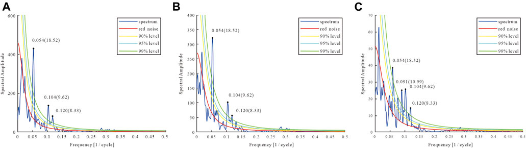
FIGURE 7. Couplet thickness variation, (A) argillaceous lamina thickness variation, and (B) sandy lamina thickness variation (C) of well A-11 after Fourier transformation in the Pinghu Formation.

The Geological Explanation of Lamina Thickness Variation

In order to characterize the effect of current cycles and sedimentary facies on the thickness of laminae quantitatively, we compared tidal cycles in various lithofacies associations and sought to identify changes in the tidal current.

Tidal Cycles in Different Lithofacies Associations

The core section of well A-11 mainly develops five sets of couplets, which are interpreted as the intertidal mixed flat, tidal channel, mud flat, mixed flat, and sand flat lithofacies associations, respectively, from bottom to top (Table 3). In the mud flat, because of more argillaceous laminae, the low preservation rate, and poor core preservation, the laminae are less recognizable, so the mud flat section is not suitable to complete the statistical calculation of the layer pair’s thickness. As a result, the sand flat, mixed flat, and tidal channel are selected for this analysis.

TABLE 3

TABLE 3. Relationship among depth, lithofacies associations, and the couplets.

On this basis, the study compared the variation of the relative content of sandy and argillaceous lamina thicknesses, discussed the variation characteristics of sandy-argillaceous couplet thicknesses in different lithofacies associations in the intertidal belt, and assessed the sedimentary environment as a whole. Near the base of the measurement section, the sedimentary environment is characterized by the transition from thick sandy and argillaceous interbeds to thin sandy and argillaceous interbeds which supports the interpretation as a mixed flat. The sandy content in the middle part increased obviously, which was manifested as the tidal channel-fill; the upper part of the argillaceous content reaches the peak value, which is mainly composed of argillaceous laminae, supporting a mud flat interpretation. Near the top of the measured section, the content of sandy and argillaceous laminae is similar, supporting the interpretation of a mixed flat setting. The sandy content of the top reaches the peak, while the argillaceous content decreases sharply, showing typical sand flat deposition (Figure 8). These characteristics further support that the variation of the sand-argillaceous couplet thickness is driven by many factors, especially the changes of tidal current deposition and lithofacies associations, while the periodic change of the sandy-argillaceous couplet thickness in tidal rhythmites can be used as a record of the tidal cycle signals.

FIGURE 8

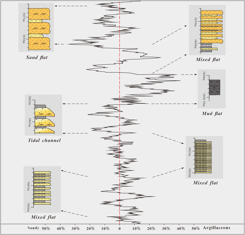
FIGURE 8. Sedimentary cycle characteristics of different lithofacies associations in well A-11 of the Pinghu Formation.

For sand flats, comparison and statistics were made on the sandy and argillaceous contents of couplets No. 1∼No. 152 (Figure 8). The percentage of the sandy content is high, and the frequency of change is low, while that of the argillaceous content is low, and the frequency of change is high. When the thickness of laminae is analyzed, the sandy laminae will weaken the tidal periodicity because of their abundance in the sand flats. Therefore, the argillaceous laminae can reflect the tidal cycles much better (Figure 8). The maximum cycle value of the thickness of the argillaceous laminae in the sand flat (Figure 9A) was verified by the red noise confidence of 99%; in other words, the spectral peak of the lowest frequency and the frequency point were 0.059. With the frequency of the peak of 0.059 as the upper limit, low-pass filtering was performed on the thickness data (Figure 9B). The filtering result of thickness is similar to a sine curve, with an average cycle of 17 laminae per interval. The lamina thickness presents a change cycle. This cycle is consistent with the maximum cycle of the argillaceous lamina thickness in well A-11 (Figure 7B), indicating that the formation of this peak is influenced by the tidal current cycle.

FIGURE 9

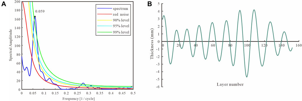
FIGURE 9. Fourier transform (A) and low-pass analysis (B) of the argillaceous thickness variation in the sand flat of well A-11 of the Pinghu Formation.

For the mixed flats, statistical analysis was run on the sandy and argillaceous contents of couplets No. 153∼No. 250 and No. 464∼No. 765 (Figure 8). The sandy and argillaceous deposits are relatively uniform, and the variation frequency of the thickness of the sandy lamina is similar to that of the argillaceous lamina (Figure 8). Therefore, the couplet thickness is selected the mixed flat section with relatively uniform sandy and argillaceous deposition. The maximum cycle value of the thickness of the couplet in the mixed flat (Figure 10A) was verified by the red noise confidence of 99%; in other words, the spectral peak of the lowest frequency and the frequency point were 0.055. With the frequency of the peak of 0.055 as the upper limit, low-pass filtering was performed on the thickness data (Figure 10B). The filtering result of thickness is similar to a sine curve, with an average cycle of 18.03 laminae per interval. This cycle is consistent with the maximum cycle of the couplet lamina thickness in well A-11 (Figure 7A), indicating that the formation of this peak is influenced by the tidal current cycle.

FIGURE 10

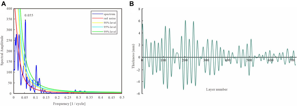
FIGURE 10. Fourier transform (A) and low-pass analysis (B) of the couple thickness variation in the mixed flat of well A-11 of the Pinghu Formation.

For the tidal channel-fill, comparison was made on the sandy and argillaceous contents of couplets No. 368∼No. 463 (Figure 8). For the tidal channel-fill, the percentage of the sandy content is large, and the frequency of change is low, while that of the argillaceous content is low, and the frequency of change is obviously high. When the thickness of laminae is analyzed, the sandy laminae will weaken the tidal periodity because of their abundance in the tidal channel. Therefore, the argillaceous laminae can reflect the tidal cycles much better (Figure 8). The maximum cycle value of the thickness of the argillaceous laminae in the tidal channel (Figure 11A) was verified by the red noise confidence of 99%; in other words, the spectral peak of the lowest frequency and the frequency point were 0.054. With the frequency of the peak of 0.054 as the upper limit, low-pass filtering was performed on the thickness data (Figure 11B). The filtering result of thickness is similar to a sine curve, with an average cycle of 18.5 laminae per interval. This cycle is consistent with the maximum cycle of the argillaceous lamina thickness in well A-11 (Figure 7B), indicating that the formation of this peak is influenced by the tidal current cycle.

FIGURE 11

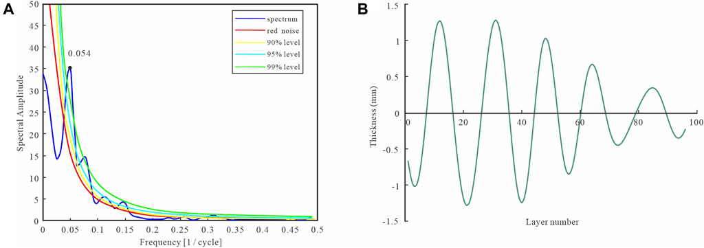
FIGURE 11. Fourier transform (A) and low-pass analysis (B) of the argillaceous thickness variation in the tidal channel of well A-11 of the Pinghu Formation.

Comparing the filtered results of both the sand flat, mixed flat, and tidal channel-fill, the trends are uniform. So the effects of the tidal cycle in the sand flat, mixed flat, and tidal channel are the same.

Facies Change in the Tidal Current

Through wavelet analysis of all couplet data in the core section, three groups of high-frequency, middle-frequency, and low-frequency data were obtained to judge the relationship between the data and lithology and sedimentary facies (Figure 12 and Figure 13). The wavelet analysis technique has been widely used to separate a time series of observations into two parts: an underlying signal or meaningful pattern of variation and a superimposed noise or random variation (Zhao et al., 2009). It can also be used to separate a time series of observations into a low-frequency variation part and a high-frequency variation part. The filtering analysis is carried out step by step. With each step, the high-frequency component is separated out, and the low-frequency components are left in the residual data. In this way, a series of components are derived with frequencies varying from high to low. The curve in Figure 11 shows that different components were distinguished from the original data through the method of wavelet analysis.

FIGURE 12

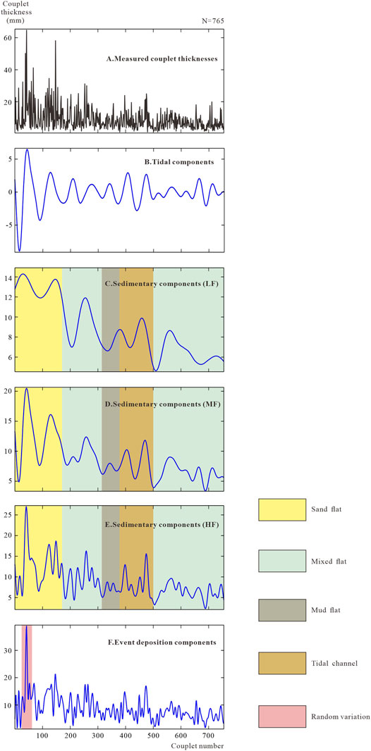
FIGURE 12. Paleotidal components, sedimentary variations and random variations derived from wavelet analysis, tidal deposits in well A-11 of the Pinghu Formation; tidal couplet sequence (N = 765). LF- relatively low-frequency sedimentary; MF- relatively middle-frequency sedimentary; HF- relatively high-frequency sedimentary. Arrowed large deviation in curve F is likely to have been caused by a storm event.

FIGURE 13

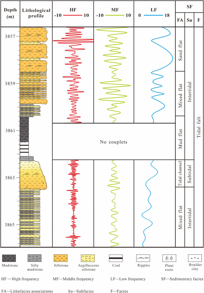
FIGURE 13. Relationship between the wavelet transform and lithofacies associations of the couplet thickness in well A-11 of the Pinghu Formation.

Curve B: Curve B presents the shape of a sine curve, showing the characteristics of the trend (Figure 12). It has a good corresponding relationship with curve A. When the couplet thickness has a crest, it is interpreted to record a spring tide, and when the couplet thickness has a trough, it is interpreted to record a neap tide.

Curves C to E: Curves C to E show that the belt of sedimentary facies becomes more obvious with the increasing frequency (Figure 12). The sand flat has the strongest energy and the largest lamina thickness. The energy and lamina thickness of the tidal channel-fill are second. The energy of the mixed flat fluctuates greatly, and the lamina thickness varies greatly. The energy of the mud flat is the most stable, and the lamina thickness is the thinnest (Figure 12 and Figure 13).

Curve F: The large deviation in curve F separated from the sand flat of curve E is likely to be caused by many factors (Figure 12), such as storms, spatial and temporal variations in megaripple dimensions, and measurement errors (Yang and Nio, 1985). However, it is unlikely that changes in megaripple dimensions would cause such abrupt changes in couplet thicknesses. It seems probable, therefore, that the large random deviations with rapid variations (e.g., the one indicated by the arrow in Figure 12, curve F) were caused by storm events. A storm tends to displace water and can be in-phase or out-of-phase with the tidal currents. After a storm, the water will seek its own equilibrium level, resulting in a reverse influence with the dominant ebb current direction, resulting in thicker tidal deposits. Since the grain size of these deposits is very coarse, storm-induced currents would have had an important influence in the transport of sediments which had a relatively high threshold of movement. Storms may not only have disturbed the regular tidal component pattern but may also have affected the regular sedimentary component pattern.

The high frequency has sawtooth peaks in the sand flat deposits (Figure 13). This may represent event deposition during storms or flooding. This is similar to Yang and Nio’s results on tidal channel bundles in 1985 (Longhitano et al., 2012). The middle frequency is nearly a sinusoidal wave, with 0.2 m in a cycle in average thickness and 18.9 laminae. This cycle is consistent with the spectrum analysis result of couplets in well A-11 (Figure 7A). Therefore, the middle-frequency signature can represent a spring-neap cycle well (Figure 13). The low-frequency signals are in good agreement with the lithofacies associations divided by the core observation (Figure 13). The curve fluctuates at the mixed flat due to the interbedding of sandy and argillaceous, and the thickness at the tidal channel increases, and the thickness at the sand flat shows the maximum peak; thus, it can be seen that high frequency reflects the event deposits’ influence, middle frequency represents the tidal effect, and low frequency is the response of lithofacies associations. Therefore, the couplets’ thickness is the combined effect of event deposits, the tidal current, and lithofacies associations.

Discussion

Preservation Potential and Periodicity for Tidal Signals

Preservation Potential

The astronomical period is a continuous time signal; however, this continuous time signal may be lost because of sedimentary discontinuity from erosion and hiatal periods. This is most evident in the tidal deposition record. In theory, a tidal cycle can be formed by at most two tidal couplets, but the number of preserved tidal cycles is quite different from the theoretical value. Many studies have shown that tidal deposits containing spring and neap tidal cycles are incomplete or poorly preserved (Yang and Nio, 1985; Li et al., 2000; Longhitano et al., 2012). The absence in the records is difficult for quantitatively assessment. The incompleteness of the tidal rhythmites may be the result of the asymmetry of the ebb and flow, the absence or erosion of the secondary tidal current, and reconstruction of waves. The tidal couplets are likely to be formed only in the dominant tidal current, and the weak secondary tidal current may not be strong enough to move the bottom sand, resulting in the absence of the corresponding sandy laminae. Moreover, Archer et al., (1995) also described in the carboniferous tidal rhythmites profile that the couplets can reflect the rising and falling tides. This was related to the characteristics of the ebb tide deposit. Our study area has weak ebb tides, with a thin sedimentary layer. It is often distributed on the upstream surface of the rising tide, which is easy to be eroded and reformed. Thus, the couplets that do preserve tend to be those deposited by the rising tidal current. Positively, this explains why only about half of the couplets can be identified from the tidal rhythmites. In addition, due to the repeated erosion of currents and the destruction of occasional storms, the sedimentary structures formed are mostly destroyed. The thickness of the tidal rhythmites that have been identified is shortened. Therefore, the number of couplets is less than that expected in continuous sedimentation.

Tidal Cycle

The tidal cycle is the smallest astronomical cycle. There are two reasons for the cycle of 18.52 laminae calculated by spectrum analysis and attributed to the tidal cycle. First, it is caused by the preservation potential of tidal couplets. This is explained in detail above. Therefore, there is a gap between the 18.52 laminae and the theoretical value of the spring-neap tide cycle. Second, it is based on previous research results (Tessier and Gigot, 1980; Visser, 1980; Yang and Nio, 1985; Williams, 1989; Kvale and Archer, 1990; Gao et al., 2000; Hovikoski et al., 2005; Zhao et al., 2008; Longhitano et al., 2012). The spring-neap tide is formed when the basic tide is strengthened or weakened under the action of the Sun’s gravity. In sediments, it often manifests as periodic changes in the thickness of the laminae or tidal bundle. During the spring tide period, due to the large tidal range and fast tidal velocity, the tidal sediments formed are also thicker. On the contrary, during the neap tide, the small tidal range and slow tidal velocity result in thinner laminae. The laminar thicknesses gradually changes from small to large or from large to small to form a “lamina cycle”, which represents a lunar semilunar tide or biweekly tide. The laminar cycle formed by the spring-neap tide deposition was identified from ancient and modern tidal sediments by Visser 1980; Tessier and Gigot, 1980; Williams, 1989; Kvale and Archer, 1990; Hovikoski et al., 2005; Longhitano et al., 2012. Generally, the number of laminae contained in the laminar cycle in the semidiurnal area is 15–30 (Wu, 1996). For example, Williams, (1989) reported that the Chambers Bluff moraine has 26.1, Tessier and Gigot, (1980) reported 25.75, Visser (1980) reported 26–30, Archer et al., (1995) reported 26, and Roep (1991) reported 27. In our analysis, we obtained the laminar cycles of 18.52 laminae, which shows the range of the number of laminae of the semidiurnal tide cycle (15–30).

Comparison With Modern and Ancient Tidal Sedimentation

Environments that are favorable to the preservation of tidal rhythmites are required for their use in high-resolution paleoenvironmental studies. In addition, field observation of the modern tidal sedimentary environment is also required to study the structure of tidal sediments and the preservation rate of couplets (Li et al., 2000).

Modern tidal sedimentation in the Rudong-Dongtai coastal area, Jiangsu province, China, is a good example (Figure 14). It can be compared with the tidal sedimentary characteristics of the Pinghu Formation in the study area. The tide has a greater impact on the coastal areas of Rudong-Dongtai. A large number of primary sedimentary structures are developed on the tidal flats, which are affected by the interplay of tides, currents, and waves. Various sedimentary structures such as ripples, deformation bedding, and slumping deformation are developed on the mud flat, and vegetation is developed. This can be compared with the phenomenon of broken cores and the development of soft sediments and root traces in the mud flat of the Pinghu Formation in the study area (Figure 15A). The mixed flat section is mainly characterized by interbedded sandy and argillaceous sediments, and relatively complete rhythmic bedding, such as wavy, vein, and lenticular bedding developed in the section, shows good stratification. This corresponds to the interbedded sandy and argillaceous sediments in the core of the mixed flat of the Pinghu Formation in the study area (Figure 15B). Sandy flats are dominated by sandy sediments, and argillaceous sediments are rare. This is analogous to the gray sandstone with ripple bedding developed in the core of the sand flat in the Pinghu Formation (Figure 15C). In the tidal channel section, it can be observed that the yellowish-brown sandy layer develops gray-white ripple bedding. This can be compared with the black-brown ripple bedding developed in the gray-white sandy layer in the core of the Pinghu Formation (Figure 15D). Therefore, the field investigation of modern sediments in the Rudong-Dongtai area of Jiangsu province, China, is of guiding significance for the restoration of the tidal sedimentary environment in the paleostratigraphic sequence of the Pinghu Formation.

FIGURE 14

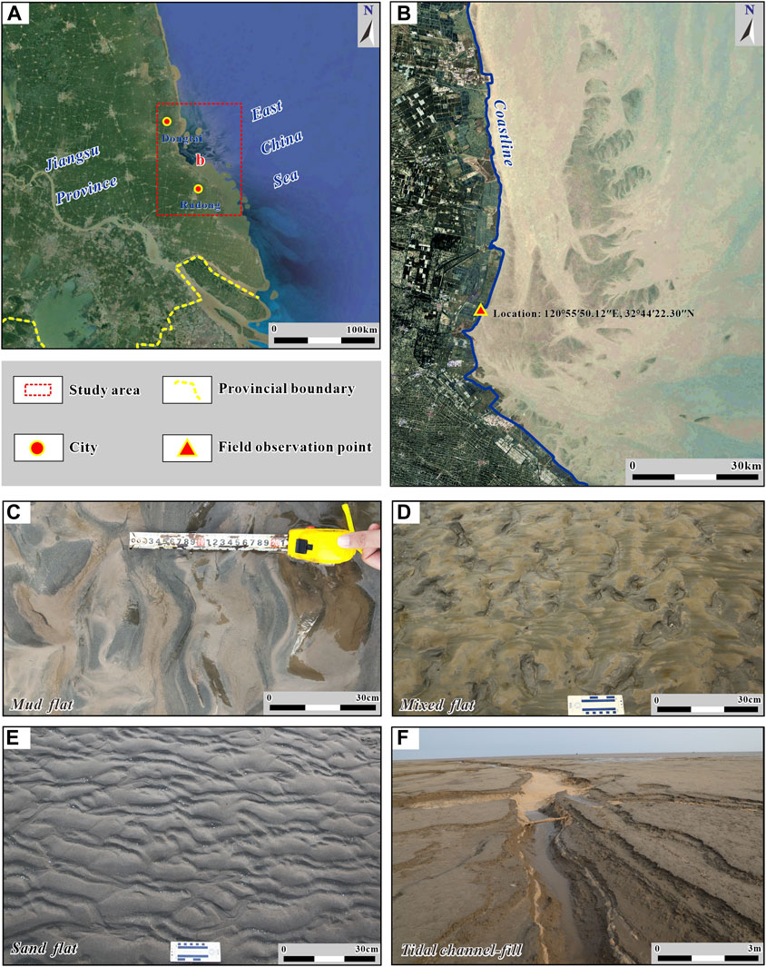
FIGURE 14. Geographical location of the modern tidal flat in the Rudong-Dongtai coastal area of Jiangsu Province, China. Within the red dotted line in (A) is the location of the modern tidal flat (B). (C–F) are modern sedimentary characteristics of the location.

FIGURE 15

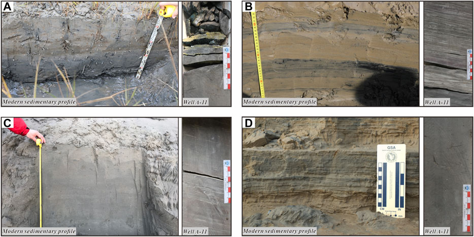
FIGURE 15. Comparison of characteristics between the modern tidal flat sedimentary profile in the Rudong-Dongtai coastal area of Jiangsu Province, China, and the well A-11 core of the Pinghu Formation in the Xihu Sag. (A) mud flat, (B) mixed flat, (C) sand flat, and (D) tidal channel-fill.

Conclusion

(1) The measurement of the thickness of sandy and argillaceous laminae is the basis for the study of tidal rhythmites. The grayscale measurement of digital images based on MATLAB is used to automatically calculate the lamina thickness of five sets of tidal rhythm development segments so as to obtain the high-resolution millimeter lamina thickness data series, and then, the periodic signals of the sedimentary rhythm were analyzed.

(2) The thickness variation of tidal rhythmites signifies the changes of lithofacies associations and the base-level cycle. Through the counting and analysis of the thickness, the tidal cycle and depositional environment variations can be summarized. It is found that the thickness variation of tidal rhythmites in the Pinghu Formation well A-11 in the Xihu Sag of the East China Sea shelf basin is the result of the comprehensive influence of event deposition, tidal current deposition, and lithofacies association change, and it is obviously manifested as the cyclic change of the tidal current cycle and lithofacies associations.

(3) Tidal couplets can record tidal signals; however, the thicknesses and numbers of this are not a simple linear relationship with tidal energy changes. In the natural tidal sedimentary environment, storm action always exists, and it can cause the distribution of couplet thicknesses and number to deviate from normal. The tidal cycle information can be removed by filtering, but it makes the interpretation of the tidal lithofacies association environment more complicated. It is necessary to analyze the more subtle variation characteristics of the tidal couplets, such as thick-thin alternation, and combine with the facies analysis to get the interpretation closer to the original sedimentary environment.

(4) Tidal rhythmites are difficult to preserve. Therefore, the method of comparative sedimentology should be applied to systematically study the areas which are favorable to the existence of tidal rhythmites in paleogeography. It provides a reference for determining the ancient rhythmic profile for tidal cycle deposition. Modern tidal sedimentation in the Rudong-Dongtai coastal area, Jiangsu province, China, is a good example. It can be compared with the tidal sedimentary characteristics of the Pinghu Formation in the study area. It is of guiding significance to restore the tidal sedimentary environment of the Pinghu Formation.

Data Availability Statement

The original contributions presented in the study are included in the article/Supplementary Material; further inquiries can be directed to the corresponding author.

Author Contributions

Conceptualization, CZ and SL; methodology, RZ and SL; software, SL; validation, SL; investigation, SL and JL; data curation, SL; writing—original draft preparation, SL; writing—review and editing, SL, JL, and ZW; visualization, SL and ZW; and supervision, CZ. All authors have read and agreed to the published version of the manuscript.

Funding

This paper was jointly supported by the National Science and Technology Major Project (No. 2016ZX05027-002-007) and the National Natural Science Foundation of China (No. 41772094).

Conflict of Interest

JL was employed by the HaiNan Branch of CNOOC China Limited.

The remaining authors declare that the research was conducted in the absence of any commercial or financial relationships that could be construed as a potential conflict of interest.

Publisher’s Note

All claims expressed in this article are solely those of the authors and do not necessarily represent those of their affiliated organizations, or those of the publisher, the editors, and the reviewers. Any product that may be evaluated in this article, or claim that may be made by its manufacturer, is not guaranteed or endorsed by the publisher.

Acknowledgments

Thank you to all those who have contributed to the research and development of tidal rhythmites over the years.

References

Abbas, A., Zhu, H., Zeng, Z., and Zhou, X. (2018). Sedimentary Facies Analysis Using Sequence Stratigraphy and Seismic Sedimentology in the Paleogene Pinghu Formation, Xihu Depression, East China Sea Shelf Basin. Mar. Pet. Geology. 93, 287–297. doi:10.1016/j.marpetgeo.2018.03.017

CrossRef Full Text | Google Scholar

Archer, A. W., Kuecher, G. J., and Kvale, E. P. (1995). The Rule of Tidal-Velocity Asymnetries in the Depxsition of Silty Tidal Thythmites (Carboniferous, Eastern Interior Coal Basin, USA). J. Sediment. rescarch 65 (2), 408.

Google Scholar

Bádenas, B., Aurell, M., Rodrı́Guez-Tovar, F. J., and Pardo-Igúzquiza, E. (2003). Sequence Stratigraphy and Bedding Rhythms of an Outer Ramp limestone Succession (Late Kimmeridgian, Northeast Spain). Sediment. Geology. 161 (1-2), 153–174. doi:10.1016/s0037-0738(03)00099-x

CrossRef Full Text | Google Scholar

Bhattacharya, B., Chakraborty, M., and Sharma, S. K. (2019). Occurrence of Tidalites in the Mesoproterozoic Subtidal-Intertidal Flat, Lalsot Sub-basin, North Delhi Fold Belt, Rajasthan, India. Aligarh, India: Springer, Cham.

Google Scholar

Chen, B., Xie, X., Al-Aasm, I., Feng, W., and Zhou, M. (2018). Depositional Architecture and Facies of a Complete Reef Complex Succession: A Case Study of the Permian Jiantianba Reefs, Western Hubei, South China. Minerals 8, 533. doi:10.3390/min8110533

CrossRef Full Text | Google Scholar

Chen, Z., Zhang, C. M., Hou, G. W., Feng, W. J., and Xu, Q. H. (2020). Fault Distribution Patterns and Their Control on Sand Bodies in Pinghu Formation of Xihu Sag in east china Sea Shelf basin. Oil Gas Geology. 41 (04), 824–837.

Google Scholar

Cheng, X., Hou, D. J., Zhou, X. H., Liu, J. S., Diao, H., Jiang, Y. H., et al. (2020). Organic Geochemistry and Kinetics for Natural Gas Generation from Mudstone and Coal in the Xihu Sag, East China Sea Shelf Basin, China. Mar. Pet. Geology. 118, 104405. doi:10.1016/j.marpetgeo.2020.104405

CrossRef Full Text | Google Scholar

Fontana, F. F., Tassios, S., Stromberg, J., Tiddy, C., van der Hoek, B., and Uvarova, Y. A. (2021). Integrated Laser-Induced Breakdown Spectroscopy (LIBS) and Multivariate Wavelet Tessellation: a New, Rapid Approach for Lithogeochemical Analysis and Interpretation. Minerals 11, 312. doi:10.3390/min11030312

CrossRef Full Text | Google Scholar

Frouin, M., Sebag, D., Laignel, B., Ogier, S., Verrecchia, E. P., and Durand, A. (2006). Tidal Rhythmites of the Marais Vernier Seine Estuary, France and Their Implications for Relative Sea-Level. Mar. Geology. 235 (1-4), 165–175. doi:10.1016/j.margeo.2006.10.012

CrossRef Full Text | Google Scholar

Gao, Z. Z., He, Y. B., Zhang, X. Y., Zhai, Y. H., Hu, Y. Y., Yang, H. J., et al. (2000). Internal-wave and Internal-Tide Deposits of the Middle-Upper Ordovician in the center Tarim basin. Acta sedimentologica sinica 03, 400–407.

Google Scholar

He, Y. P. (2020). Discovery and Geological Significance of Eocene Pinghu Formation Tempestites in Tiantai Area,Xihu Sag,East China Sea Basin. J. Jilin University(Earth Sci. Edition) 50 (2), 500–508.

Google Scholar

Hovikoski, J., Räsänen, M., Gingras, M., Roddaz, M., Brusset, S., Hermoza, W., et al. (2005). Miocene semidiurnal tidal rhythmites in Madre de Dios, Peru. Geol 33 (3), 177–180. doi:10.1130/g21102.1

CrossRef Full Text | Google Scholar

Jiang, H. J., Hu, M. Y., Hu, Z. G., Ke, L., Xu, Y. X., and Wu, L. Q. (2011). Sedimentary Environment of Paleogene in Xihu Sag: Microfossil as the Main Foundation. Lithologic reservoirs 23 (1), 74–78.

Google Scholar

Jiang, Y. M., Shao, L. Y., Li, S., Zhao, H., Kang, S. L., Shen, W. C., et al. (2020). Deposition System and Stratigraphy of Pinghu Formation in Pinghu Tectonic Belt, Xihu Sag. Geoscience 34 (01), 141–153.

Google Scholar

Kvale, E. P., and Archer, A. W. (1990). Tidal Deposits Associated with Low-Sulfur Coals, Brazil Fm. (Lower Pennsylvanian), Indiana. J. Sediment. Pet. 60 (4), 563–574. doi:10.1306/212f91e7-2b24-11d7-8648000102c1865d

CrossRef Full Text | Google Scholar

Kvale, E. P., Johnson, H. W., Sonett, C. P., Archer, A. W., and Zawistoski, A. (1999). Calculating Lunar Retreat Rates Using Tidal Rhythmites. J. Sediment. Res. 69 (6), 1154–1168. doi:10.2110/jsr.69.1154

CrossRef Full Text | Google Scholar

Li, C., Wang, P., Daidu, F., Bing, D., and Tiesong, L. (2000). Open-coast Intertidal Deposits and the Preservation Potential of Individual Laminae: a Case Study from East-central China. Sedimentology 47, 1039–1051. doi:10.1046/j.1365-3091.2000.00338.x

CrossRef Full Text | Google Scholar

Li, X., Fan, Y. R., Yang, L. W., and Fang, W. J. (2006). Application of Wavelet Inversion Characteristics of Logging Curve in the Classification of Sequence Stratigraphy. Pet. Geology. oilfied Dev. daqing 04, 112–115+126.

Google Scholar

Liu, S. H., Wang, B. Y., and Liu, C. X. (2009). Petroleum Geology and Recovery Efficiency. Pet. Geology. recovery efficiency 16 (03), 1–3+113.

Google Scholar

Longhitano, S. G., Mellere, D., Steel, R. J., and Ainsworth, R. B. (2012). Tidal Depositional Systems in the Rock Record: A Review and New Insights. Sediment. Geology. 279 (20), 2–22. doi:10.1016/j.sedgeo.2012.03.024

CrossRef Full Text | Google Scholar

Lopes, M., Amorim, A., Calado, C., and Reis Costa, P. (2018). Determination of Cell Abundances and Paralytic Shellfish Toxins in Cultures of the Dinoflagellate Gymnodinium Catenatum by Fourier Transform Near Infrared Spectroscopy. Jmse 6, 147. doi:10.3390/jmse6040147

CrossRef Full Text | Google Scholar

Roep, T. B. (1991). Neap-spring Cycles in a Subrecent Tidal Channel Fill (3665 BP) at Schoorldam, NW Netherlands. Sediment. Geology. 71 (3-4), 213–230. doi:10.1016/0037-0738(91)90103-k

CrossRef Full Text | Google Scholar

Santos, D., Abreu, T., Silva, P. A., and Baptista, P. (2020). Estimation of Coastal Bathymetry Using Wavelets. Jmse 8, 772. doi:10.3390/jmse8100772

CrossRef Full Text | Google Scholar

Tessier, B., and Gigot, P. (1980). A Vertical Record of Different Tidal Cyclicities:an Example from the Miocene marine Molasses of Digne(Haute Provance, France). Sedimentology 6, 767–776.

Google Scholar

Visser, M. J. (1980). Neap-spring Cycles Reflected in Holocene Subtidal Large-Scale Bedform Deposits: A Preliminary Note. Geol 8 (11), 543–546. doi:10.1130/0091-7613(1980)8<543:ncrihs>2.0.co;2

CrossRef Full Text | Google Scholar

Williams, G. E. (1989). Late Precambrian Tidal Rhythmites in South Australia and the History of the Earth's Rotation. J. Geol. Soc. 146, 97–111. doi:10.1144/gsjgs.146.1.0097

CrossRef Full Text | Google Scholar

Wu, J. P., Wan, L. F., Zhang, L., Wang, Y. M., Zhao, Q. H., Li, K., et al. (2017). Lithofacies Types and Sedimentary Facies of Pinghu Formation in Xihu Depression. Lithologic reservoirs 29 (01), 27–34.

Google Scholar

Wu, X. F., Yi, H. S., Huan, Y. L., Xia, G. Q., and Hui, B. (2012). A New Method for Calculating Tidal Sedimentary Rhythm and its Application: a Case Study of the Algal Dolomite Laminae from Middle Triassic Leikoupo Formation, Jiangyou Area, Sichuan Province. Geol. Bull. china 31 (05), 758–762.

Google Scholar

Wu, Z. Y. (1994). A Study on the Tidal Periodicities and its Im-Plications. Geol. Sci. Technol. Inf. 03, 57–62.

Google Scholar

Wu, Z. Y. (1996). Advance in the Tidal Rhythmites and its Implications for the Astro-Geology. Prog. Geophys. 11 (4), 100–111.

Google Scholar

Yang, C.-S., and Nio, S.-D. (1985). The Estimation of Palaeohydrodynamic Processes from Subtidal Deposits Using Time Series Analysis Methods. Sedimentology 32, 41–57. doi:10.1111/j.1365-3091.1985.tb00491.x

CrossRef Full Text | Google Scholar

Yang, C. H., Gao, Z. Z., Jiang, Y. M., and Gao, W. Z. (2013). Reunderstanding of Clastic Rock Sedimentary Facies of Eocene Pinghu Formation in Pinghu Slope of Xihu Sag. J. oil gas Technol. 35 (09), 11–14+1.

Google Scholar

Yi, H. S. (2012). Detection of Cyclostratigraphic Sequence Surfaces in Stratigraphic Record:Its Principle and Approach. Acta Sedimentologica Sinica 30 (06), 991–998.

Google Scholar

Yi, H. S., Shi, Z. Q., Yang, W., and Hui, B. (2010). Astroncmical Periodicity Signals Form Lamina Growth Rhythm Records of Lacustrine Stromatolites. Acta sedimentologica sinica 28 (03), 405–411.

Google Scholar

Yu, X. H., Li, S. L., Cao, B., Hou, G. W., Wang, Y. F., and HuangFu, Z. Y. (2017). Oligocene Sequence Framework and Depositional Response in the Xihu Depression, East China Sea Shelf Basin. Acta Sedimentologica Sinica 2017 (02), 299–314.

Google Scholar

Zhao, H., Jiang, Y. M., Chang, Y. S., Li, S., and Li, J. (2018). Study on Sedimentary Characteristics of the Pinghu Formation Based on Sedimentary Facies Markers in Xihu Sag, east china Sea basin. Shanghai land Resour. 39 (01), 88–92.

Google Scholar

Zhao, L. N. (2007). The Study on Sedimentary Facies of Pinghu Zone in Xihu Sag in the east china Sea Shelf basin. Master’s thesis. Jilin, China: Jinlin university.

Google Scholar

Zhao, W., Qiu, L. W., Jiang, Z. X., and Chen, Y. (2009). Application of Wavelet Analysis in High-Resolution Sequence Unit Division. J. china Univ. Pet. 33 (02), 18–22.

Google Scholar

Zhao, X. F., Lv, Z. G., Zhang, W. L., Peng, H. R., and Kang, R. D. (2008). Paralic Tidal Deposits in the Upper Triassic Xujiahe Formation in Anyue Area,the Sichuan basin. Nat. gas industry 04, 14–18+134.

Google Scholar

Zhou, Y. Q., Chen, H. Y., and Ji, G. S. (2002). Tidal Rhythmites in Cambrian-Ordovician,north china and Evolution of Orbit Parameters. Earth Sci. 06, 671–675.

Google Scholar

Zhu, R., Zhang, C. M., Zhang, S. F., Shi, H., Du, J., and Yu, Y. (2010). Thickness Variation of Tidal Couplets and its Geological Significance. Mar. Geology. Quat. Geology. 30 (06), 9–14.

Google Scholar