TOC interpretation of lithofacies-based categorical regression model: A case study of the Yanchang formation shale in the Ordos basin, NW China

In this paper, taking the shale of Chang 7-Chang 9 oil formation in Yanchang Formation in the southeastern Ordos Basin as an example, through the study of shale heterogeneity characteristics, starting from the preprocessing of supervision data set, a logging interpretation method of total organic carbon content (TOC) on the lithofacies-based Categorical regression model (LBCRM) is proposed. It is show that: 1) Based on core observation, and Differences of sedimentation and structure, five lithofacies developed in the Yanchang Formation: shale shale facies, siltstone/ultrafine sandstone facies, tuff facies, argillaceous shale facies with silty lamina and argillaceous shale facies with tuff lamina. 2) The strong heterogeneity of shale makes it difficult to accurately explain the TOC distribution of shale intervals in the application of model-based interpretation methods. The LBCRM interpretation method based on the understanding of shale heterogeneity can effectively reduce the influence of formation factors other than TOC on the prediction accuracy by studying the characteristics of shale heterogeneity and constructing a TOC interpretation model for each lithofacies category. At the same time, the degree of unbalanced distribution of data is reduced, so that the data mining algorithm achieves better prediction effect. 3) The interpretability of lithofacies logging ensures the wellsite application based on the classification and regression model of lithofacies. Compared with the traditional homogeneous regression model, the prediction performance has been greatly improved, TOC segment prediction is more accurate. 4) The LBCRM method based on shale heterogeneity can better understand the reasons for the deviation of the traditional model-based interpretation method. After being combined with the latter, it can make logging data provide more useful information.

1 Introduction

Organic matter content is an indispensable basic data for source rock evaluation, shale oil and gas reservoir evaluation and sweet spot prediction. (Curtis, 2002; Passey et al., 2010; Sondergeld et al., 2010; Alfred and Vernik, 2012; Ma, 2015; Altowairqi et al., 2015; Aldrich and seidle, 2018; Guo et al., 2021; Wei et al., 2021; Meng, 2022). Laboratory core test and analysis technology is the most direct and accurate means to obtain the organic matter content of shale, in which total organic carbon content (TOC) is the most readily available and commonly used characterization index of organic matter content. Restricted by the lack of core data or incomplete coring in most wells, the interpretation of formation TOC with high resolution and high coverage logging data is an important means for rapid, accurate and continuous quantitative evaluation of organic matter content in shale formations (Yu et al., 2017; Wang et al., 2019; Liang et al., 2021; Chan et al., 2022; Meng et al., 2022; Zhao et al., 2022).

At present, a large number of TOC logging interpretation methods, techniques or models have been proposed. These methods can be divided into two categories: model-driven and data-driven (Huang and Williamson, 1996). Model-driven methods include formation density curve method (Schmoker, 1979; Schmoker and Hester, 1981), natural gamma intensity method (Schmoker, 1981; fertl and Chilinger, 1988), I-x method (Dellenbach et al., 1983), ΔlogR and its improved method (Passey et al., 1990; wang et al., 2016; zhao et al., 2017), CARBOLOG (Carpentier et al., 1991), etc. This type of method constructs a statistical relationship between logging response and TOC through specific assumptions (Sondergeld et al., 2010). For example, the formation density curve and the natural gamma intensity method construct the TOC logging interpretation method through the linear volume equation of the logging response (Huang and Williamson, 1996), and the ΔlogR establishes the non-linear relationship between the ΔlogR and the TOC by obtaining the superposition baseline of the porosity curve and the resistivity curve at the pure water-bearing non-hydrocarbon source rock under the premise of the known shale mature section (Passey et al., 1990; 2010).

Huang and Williamson (1996) pointed out that the model-driven method need to determine the key parameter to accurately estimate the organic matter content of the shale section. The above drawbacks restrict the application of model-driven methods in the interpretation of organic matter content and promote the development of data-driven methods (Huang and Williamson, 1996). Different from the model-driven method, the data-driven method can fully explore the statistical relationship between multi-logging response characteristics and TOC, which is more suitable for TOC interpretation of strongly heterogeneous shale (Huang and Williamson, 1996). Currently, a large number of data mining algorithms have been applied to TOC logging interpretation, including multiple linear regression, Gaussian mixture, optimization algorithm, SVM, BP neural network, deep neural network, etc., (Mendelzon and Roksoz, 1985; Huang and Williamson, 1996; Wang et al., 2014; Tan et al., 2015; Yu et al., 2017; Zhu et al., 2020; Zheng et al., 2021; Chan et al., 2022).

In the data-driven TOC interpretation technology, there are two challenges: First, the formation logging response is not only affected by TOC, but also by multi-formation factors such as particle size, mineral composition, element composition, pore development degree, pore fluid properties, etc., resulting in the logging response and organic matter content is not a simple linear relationship (Huang et al., 1996; yang et al., 2004; rezaee et al., 2007). The above characteristics have caused a prominent problem, whether the conventional logging series can provide sufficient features to make the TOC interpretation have high enough accuracy, in other words, in the formation with the same or similar logging response, whether the samples have different TOC values. Chan et al. (2020) showed that the accuracy of TOC interpretation based solely on conventional logging series may not be ideal. The TOC deep learning interpretation model constructed by adding element information to conventional logging series data is significantly better than the results of Mahmoud et al. (2017) that rely solely on conventional logging prediction models (Chan et al., 2020). It can be seen that the simple introduction of more complex machine learning algorithms cannot completely solve the accurate interpretation of TOC. It is also necessary to understand the above problems from the perspective of data characteristics, which is particularly important in shale oil and gas reservoirs with strong heterogeneity of lithology, mineral composition and elemental composition.

Another problem comes from the data mining algorithm itself. In all data-driven TOC interpretation methods, the goal is to minimize the difference between the predicted value and the true value of the expected value (such as MSE and RMSE, etc.) (Huang and Williamson, 1996; Wang et al., 2014; Tan et al., 2015; Yu et al., 2017; Zhu et al., 2020; Zheng et al., 2021; Chan et al., 2022), which is the most direct indicator of learning algorithms in model training and performance verification. However, TOC test samples are often sampled by equidistant or random methods. The strong heterogeneity of shale inevitably causes some TOC numerical interval samples to be more concentrated. The TOC data exhibit skewed distribution with a long tail (Yu et al., 2019; Wang et al., 2012), causing an imbalance in data distribution (Branco et al., 2016). The learning goal of minimizing the expected difference makes the learning algorithm pay more attention to the characteristics of high-frequency distribution samples, resulting in lower prediction accuracy for data with a small number of samples (Branco et al., 2016; 2018). Unfortunately, the TOC interval with low data density may be the focus of shale reservoir research, such as shale sections with high TOC distribution. At present, the application of learning algorithms in imbalanced data is still less involved in regression problems such as TOC logging interpretation (Branco et al., 2016; 2018).

In view of the above problems, this paper takes Yanchang Formation in Ordos Basin as the research object, and proposes a logging interpretation method of organic carbon content based on rock facies classification regression model (LBCRM) from the preprocessing of supervised data sets. This method adds an additional dimension of lithofacies to the TOC-logging response monitoring data set through the study of shale heterogeneity characteristics. The TOC interpretation sub-model based on SVM algorithm is constructed by classification, which effectively reduces the influence of formation factors other than TOC on TOC interpretation accuracy. At the same time, the degree of unbalanced data distribution is reduced, which makes the data mining algorithm achieve better prediction results. XGboost can be used to construct a high-precision rock facies logging identification method, which ensures the availability of rock facies and makes this method have practical application potential. In addition, based on the analysis of heterogeneity characteristics, the interpretation results of this method can also be combined with the traditional model-driven method to obtain more formation parameters.

2 Materials

This study is based on the Yanchang Formation shale in the southeastern Ordos Basin (Figure 1A). The shale is a Triassic continental deposit, and the mud shale section is located in the Chang 7 ∼ Chang 9 oil formation. The data come from core samples and conventional logging curves of 12 wells (Figure 1B). As shown in Table 1, based on the core description of the above 12 wells, the samples were selected for TOC, mineral composition, extraction and pyrolysis test, and the core homing work was carried out.

FIGURE 1

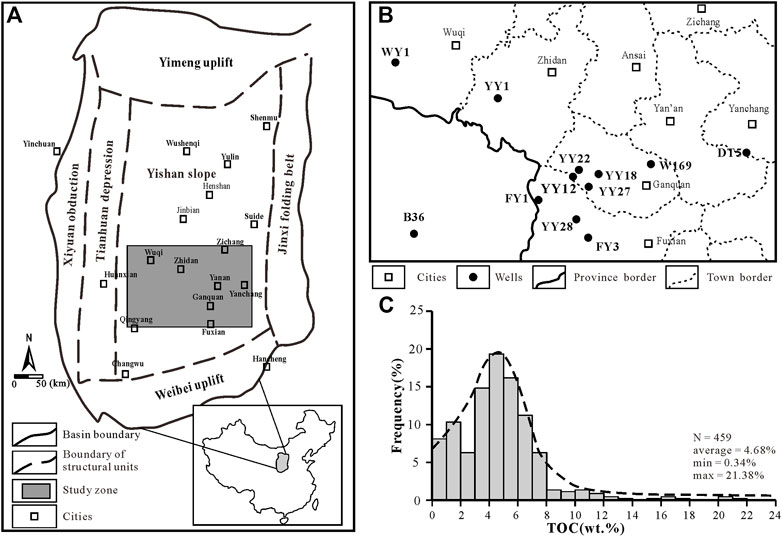
FIGURE 1. (A) Location of Ordos Basin and study area (modified by Yang et al., 2005); (B) Horizontal distribution of wells in the study area; (C) TOC frequency distribution histogram.

TABLE 1

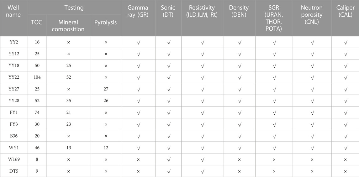
TABLE 1. Testing data and conventional well logs used in this study.

Among them, the TOC sample size is 459. Statistics show that the TOC distribution is 0.34 wt%∼29.11 wt% (4.76% on average). From Figure 1C, it can be found that the data exhibit skewed distribution with a long tail. The high-density data distribution area is located at 3 wt% ∼ 8 wt%, showing that the data has an unbalanced distribution (Buda et al., 2018; Liu et al., 2019).

In addition to the TOC test, the whole rock mineral composition and pyrolysis test were also carried out in this study. These data were used to illustrate the differences in mineral composition and oil content of different lithofacies.

Except W169 and DT5 wells which lack Density, SGR and Neutron logging series, 10 wells have complete logging series. In this study, the 10 wells were selected to construct the LBCRM method, W169 and DT5 were used for the extended application of the LBCRM method.

3 Methodology

3.1 Principle of LBCRM

In essence, data-driven TOC logging interpretation is a typical data regression problem based on learning algorithms. Suppose that a supervised data set $D_t={\left\{\left(x_i,y_i\right)\right\}}_{i=1}^n$, where x∈X, y∈Y, is derived from the joint distribution P_{X × Y}. The goal of the data-driven method is to establish a mapping relationship f∈F:X ->Y, such that the expected error ${\epsilon }_{ex}=E_{\left(x,y\right)\sim P_{X\times Y}}L\left(f\left(x\right),y\right)$ is minimized, where L (f (x), y) is the loss function, representing the difference between the predicted value f (x) and the supervised target y value. In practice, the joint distribution P_{X × Y} is unknown, x and y generally take values from the supervised data set D_t, so the objective of the regression problem is to minimize ${\epsilon }_{em}=E_{\left(x,y\right)\sim D_t}L\left(f\left(x\right),y\right)$. When the supervised data set is large enough, ε = |ε_ex-ε_em| is small enough, so that the regression fitting relationship f has better prediction effect. For logging interpretation, x is the conventional logging response, f is the formation characteristic parameters, including mineral composition, element composition and organic matter content.

Compared with the easily available TOC data, other formation parameter data are often difficult to obtain for various reasons. Therefore, the target output in the supervised data set D_t of TOC logging interpretation is only TOC data. This requires that conventional logging responses can provide sufficient differentiated features to distinguish TOC values. A comparative study by Chan et al. (2020) and Mahmoud et al. (2017) found that prediction accuracy can be significantly improved by adding dimensional information to conventional logging responses, suggesting that conventional logging responses may not be sufficient to provide complete features for accurate interpretation of TOC.

Similar to Chan et al. (2020), the TOC interpretation model based on rock facies classification and regression improves the prediction accuracy of TOC by adding additional dimension information to logging information. Based on the study of shale heterogeneity, this method constructs a relatively homogeneous lithofacies unit and uses it as additional information to constrain TOC interpretation. The mathematical expression of the regression target of this method is to divide the D_t data set into m subsets $D_t^m$, and establish a function mapping relationship f_j for each subset to minimize Eq. 1:

${\epsilon }_{em}={\displaystyle \sum }_{j=1}^m{\epsilon }_{em}^j={\displaystyle \sum }_{j=1}^m{E}_{\left(x,y\right)\sim D_t^j}L\left(f\left(x\right),y\right),(1)$

where m is the number of types of lithofacies units,j∈ [1.2,…m].

Figure 2 shows the basic idea of this method. Traditional data-driven TOC interpretation methods use a uniform regression model (URM) when constructing prediction models. As shown in Figure 2A, firstly, the homogeneous regression model ignores that the input data is not enough to provide enough differentiated features to describe the output target. Secondly, the data imbalance in the supervised data makes the learning algorithm have the data characteristics in the rectangular area in Figure 2B, but the fitting model in Figure 2A cannot have good prediction performance for the data outside the gray rectangular area. The classification fitting regression model shown in Figure 2C can increase the type dimension information, so that the learning algorithm can obtain a more accurate prediction model in the data within different categories. At the same time, as shown in Figure 2D, this method can also reduce the imbalance of the data, so that the learning algorithm will not only focus on the data with high frequency distribution, especially for the high density of local data distribution caused by the coincidence of different types of data.

FIGURE. 2

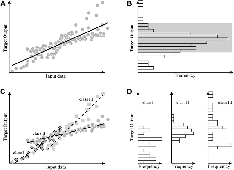
FIGURE. 2. Schematic diagram of regression prediction model based on rock facies classification (A) The effect of using a uniform regression fitting model in the case of incomplete input data and unbalanced supervised data; (B) The unbalanced distribution characteristics of the data set; (C) The effect of using classification fitting regression fitting model in the case of incomplete input data and unbalanced supervised data; (D) classification fitting regression subdataset imbalance distribution reduction.

3.2 Classification of lithofacies

At present, the classification of shale rock facies is mainly divided into two categories. One is based on the difference of sedimentary and structure on the core scale of mud shale section (Singh et al., 2008; Zhen et al., 2016; Kristen, 2015; Long et al., 2022; Zhang et al., 2022); the second is based on rock physics parameters, especially mineral composition parameters (Wang et al., 2012; Gao et al., 2018; Ou et al., 2018; Schlanser, 2015).

In this study, the rock has three corresponding characteristics. One is that the rock facies type is not easy to be too complicated for the consideration of well site application, which makes it difficult to establish a logging identification method with high prediction accuracy. The second is easy to obtain. On the one hand, it is conducive to the formation of large-scale data sets, on the other hand, the rock type classification using TOC data; The third is the thickness of rock facies should be above the vertical resolution of the logging. Taking DEN with the highest vertical resolution in conventional logging as an example, the thickness of rock facies should be at least 30 cm.

Due to the numerous petrophysical parameters affecting the logging response, a more complex classification scheme will be formed in the rock facies construction, and it is easy to fall into the rock facies classification only for TOC data with petrophysical parameters. Therefore, this study uses the difference of sedimentary and structure on the core scale as the basis for the division of rock facies. At the same time, in order to avoid the occurrence of complex lithofacies types, only the sedimentary characteristics that have obvious influence on rock physics characteristics are considered. In addition, in order to correspond to the vertical resolution of logging, the thickness of a single rock facies layer is at least 30 cm.

3.3 Machine learning method

The data mining algorithms used in this study include SVR (support vector machine) and XGboost. In addition, genetic algorithm is used to optimize the hyperparameters of the above two algorithms, and K-fold cross validation is used to improve the generalization ability of the training model.

3.3.1 SVR method

SVR has incomparable advantages in data mining of small sample data sets. Considering that there may be a small amount of data in some data sets after the construction of sub-data sets, this paper chooses SVR as the basic data mining algorithm for TOC logging interpretation. The basic concept of SVR method is to project the input data into a higher dimension by kernel function, so as to find a hyperplane to establish a regression function. For a given data set {(x₁,y₁),……, (x_l,y_l) }, where x_i∈Rⁿ is the input data, y_i∈R¹ is the target output value, and the SVR estimation function is:

$f\left(x\right)=w^{\mathrm{T}}·\mathrm{\Phi }\left(\mathrm{x}\right)+b,(2)$

where w and b are hyperplane parameters, Φ(x) denotes the eigenvectors after x projection. The standard form of SVR for solving hyperplane parameters is (Vapnik, 1998):

$\begin{array}{c}\mathbf{min}\\ w,b,\xi ,{\xi }^{*}\end{array}\frac{1}{2}{w}^{T}w+C{\displaystyle \sum }_{i=1}^l\left({\xi }_i+{\xi }_i^{*}\right).(\mathrm{3a})$

受制于.

Subject to

$w^T·\mathrm{\Phi }\left(x_i\right)+b-y_i\le \epsilon +{\xi }_i,(\mathrm{3b})$

$y_i-w^T·\mathrm{\Phi }\left(x_i\right)-b\le ϵ+{\xi }_i^{*},$

${\xi }_i,{\xi }_i^{*}\ge 0,i=1,\cdots ,l,$

where C is the penalty coefficient or regularization parameter, and ε, ξ,ξ*∈R are slack variables introduced to penalize the fitting function. Eq. 1 can be transformed into a dual problem to solve, and the original problem is transformed into its corresponding Lagrangian function form, and by minimizing:

$\begin{array}{c}\mathbf{min}\\ \alpha ,{\alpha }^{*}\end{array}\frac{1}{2}{\displaystyle \sum }_{i=1}^l{\displaystyle \sum }_{j=1}^l\left({\alpha }_i-{\alpha }_i^{*}\right)\left({\alpha }_j-{\alpha }_j^{*}\right)K\left(x_i,x_j\right)+\epsilon {\displaystyle \sum }_{i=1}^l\left({\alpha }_i+{\alpha }_i^{*}\right)+{\displaystyle \sum }_{i=1}^l{y}_i\left({\alpha }_i-{\alpha }_i^{*}\right).(\mathrm{4a})$

Subject to

${\displaystyle \sum }_{i=1}^l\left({\alpha }_i-{\alpha }_i^{*}\right)=0,(\mathrm{4b})$

$0\le {\alpha }_i,{\alpha }_i^{*}\le C,i=1,\cdots ,l,$

where α_i = (α₁, α₂,…α_l) is the Lagrange multiplier, and K (x_i,x_j) is the kernel function. The final regression equation is:

$f\left(x\right)={\displaystyle \sum }_{i=1}^n\left({\alpha }_i-{\alpha }_i^{*}\right)K\left(x_i,x_j\right)+b.(5)$

In this paper, polynomial kernel function, radial basis kernel function (RBF) and sigmod kernel function are selected to explain TOC respectively, so as to optimize the best kernel function type.

3.3.2 XGboost

XGboost was first proposed by Chen and Guestrin (2016). It is a machine learning algorithm that relies on the boosting principle and explores weak learners to comprehensively predict. This is mainly due to its well-known high prediction accuracy. Its basic principle is to generate a sub-classifier to fit the prediction residuals of the previous sub-classifiers, thereby continuously reducing the residuals between the true value and the predicted value, and finally integrating all sub-classifiers to give the final prediction result. The expression is:

${\widehat{y}}_i={\displaystyle \sum }_{k=1}^K{f}_k\left(x_i\right),f_k\in F.(6)$

Among them, ${\widehat{y}}_i$ is the calculated predictive value of the i th sample; K denotes the number of decision trees; f_k denotes the kth submodel; x_i represents the input feature of the ith sample; F represents the set of sub-classifiers. In the Xgboost sub-classifier, the Classification and Regression Tree is usually selected. In the Xgboost algorithm, the objective function is composed of a loss function and regularization parameters. The expression is:

$\mathrm{L}\left(\phi \right)={\displaystyle \sum }_{i}l\left({\widehat{y}}_i,y_i\right)+{\displaystyle \sum }_k\mathrm{\Omega }\left(f_k\right),where\mathrm{\Omega }\left(f\right)=\gamma T+\frac{1}{2}\lambda {‖w‖}^2.(7)$

Among them, $l\left({\widehat{y}}_i,y_i\right)$ is the residual between the predicted value ${\widehat{y}}_i$ and the target value y_i; f_k is the function expression of the k sub-classifier; $\Omega \left(f_k\right)$ is the penalty term of the model complexity, which can be used to smooth the final learned weights to avoid overfitting. XGboost is trained iteratively to obtain an approximation of L(φ). Assuming that the sub-classifier trained in the t iteration is f_t, after the t iteration, the objective function can be expressed as:

$L^t={\displaystyle \sum }_{i=1}^{n}l\left({\widehat{y}}_i^{t-1}+f_t\left(x_i\right),y_i\right)+\mathrm{\Omega }\left(f_k\right).(8)$

Equation. 8 can be further optimized using second-order approximation:

$L^t\cong {\displaystyle \sum }_{i=1}^n\left[l\left({\widehat{y}}_i^{t-1},y_i\right)+g_i{f}_t\left(x_i\right)+\frac{1}{2}{h}_i{f}_t^2\left(x_i\right)\right]+\mathrm{\Omega }\left(f_k\right),(9)$

where, g_i and h_i are the first-order and second-order partial derivatives (gradients) of l, respectively, where $g_i={\partial }_{{\widehat{y}}^{t-1}}l\left({\widehat{y}}_i^{\left(t-1\right)},y_i\right)$ 和 $h_i={\partial }_{{\widehat{y}}^{t-1}}^{2}l\left({\widehat{y}}_i^{\left(t-1\right)},y_i\right)$. After taking them into Eq. 9 and removing the constant term, we can obtain:

${\stackrel{\sim }{\mathrm{L}}}^t={\displaystyle \sum }_{i=1}^n\left[g_i{f}_t\left(x_i\right)+\frac{1}{2}{h}_i{f}_t^2\left(x_i\right)\right]+\mathrm{\Omega }\left(f_t\right).(10)$

Define I_j={i | q (x_i) = j} as an instance set of leaf node j. Eq. 10 is rewritten by extending Ω to:

${\stackrel{\sim }{\mathrm{L}}}^t={\displaystyle \sum }_{i=1}^n\left[g_i{f}_t\left(x_i\right)+\frac{1}{2}{h}_i{f}_t^2\left(x_i\right)\right]+\gamma T+\frac{1}{2}\lambda {\displaystyle \sum }_{j=1}^T{w_j}^2={\displaystyle \sum }_{j=1}^n\left[\left({\displaystyle \sum }_{i\in I_j}{g}_i\right)w_j+\frac{1}{2}\left({\displaystyle \sum }_{i\in I_j}{h}_i+\lambda \right)w_j^2\right]+\gamma T.(11)$

Therefore, the objective function is transformed into a function of the first and second partial derivatives of the loss function l, the leaf node weight, and the number of leaf nodes. In the case of fixed tree structure q(x) the optimal weight w_j*of leaf node j can be calculated by the following formula:

$w_j^{*}=-\frac{{\displaystyle \sum }_{i\in I_j}{g}_i}{{\displaystyle \sum }_{i\in I_j}{h}_i+\lambda }.(12)$

The optimal solution formula of the objective function is as follows:

${\stackrel{\sim }{\mathrm{L}}}^t\left(q\right)=-\frac{1}{2}{\displaystyle \sum }_{j=1}^T\frac{{{\displaystyle \sum }_{i\in I_j}{g}_i}^2}{{\displaystyle \sum }_{i\in I_j}{h}_i+\lambda }+\gamma T.(13)$

XGboost iteratively adds branches to construct sub-classifiers on the initial leaf nodes through a greedy algorithm to determine the optimal tree structure of the CART tree. Suppose there is a leaf node, I_L and I_R are instances of the left and right nodes after the node is branched. Let I = I_L∪I_R, then the loss after branching is reduced to:

${\mathrm{L}}_{split}=\frac{1}{2}\left[\frac{{{\displaystyle \sum }_{i\in I_L}{g}_i}^2}{{\displaystyle \sum }_{i\in I_L}{h}_i+\lambda }+\frac{{{\displaystyle \sum }_{i\in I_R}{g}_i}^2}{{\displaystyle \sum }_{i\in I_R}{h}_i+\lambda }-\frac{{{\displaystyle \sum }_{i\in I}{g}_i}^2}{{\displaystyle \sum }_{i\in I}{h}_i+\lambda }\right]-\gamma .(14)$

If L_split is greater than 0, the objective function decreases after the leaf node is split into two leaf nodes, so as to determine the node segmentation. On this basis, XGboost is optimized by feature pre-ranking, quantile approximation, and parallel lookup to quickly find the nearest split point.

3.3.3 Genetic algorithm

In the SVM and XGboost algorithm, there are a large number of hyper-parameters, which will affect the final prediction results. Therefore, it is necessary to use hyper-parameter optimization algorithm to determine which hyper-parameter system the SVM and XGboost algorithm can achieve the best prediction results. This study used Genetic Algorithm to optimize hyperparameters.

Genetic algorithm was first proposed by Holland (1973). It is a parallel stochastic optimization algorithm developed from the simulation of natural genetic mechanism and biological evolution theory. The genetic algorithm starts with a set of randomly generated parameters to be optimized, which is called the initial population, where each parameter pair is called an individual. Genetic algorithm encodes each individual in series to form chromosome, and determines the fitness function according to the optimization objective to calculate the fitness of each individual. Several individuals with high fitness values are selected from the initial population, and the chromosomes encoded by these individuals are crossed and mutated to form a new generation of individual populations. Then the fitness of each individual in the new population is calculated, and the above operations are performed repeatedly until the target value or the maximum number of iterations satisfying the fitness is met. In the iterative process, the genetic algorithm can preserve the individuals with good fitness values and eliminate the individuals with poor fitness. The new population not only inherits the information of the previous generation, but also is superior to the previous generation. Through continuous iteration, the parameters can be optimized.

3.4 Evaluation metics systems

In order to evaluate the predictive performance of the model, four evaluation indicators were used in this study, including RMSE, R2, MAE, MAPE, Mlogloss and Confusion matrix. The first four indexes are used to evaluate the prediction performance of TOC, and the latter two are used to evaluate the accuracy of rock facies identification.

$RMSE=\sqrt{\frac{1}{n}{\displaystyle \sum }_{i=1}^n{\left(y_i-{\widehat{y}}_i\right)}^2},(15)$

$MAE=\frac{1}{n}{\displaystyle \sum }_{i=1}^n\left|y_i-{\widehat{y}}_i\right|,(16)$

$MAPE=\frac{1}{n}{\displaystyle \sum }_{i=1}^n\frac{\left|y_i-{\widehat{y}}_i\right|}{y_i},(17)$

Among them, y_i represents the true value of TOC, ${\widehat{y}}_i$ is the predicted value of TOC, and n represents the number of TOC data. The lower the value of the above index represents the better performance of the prediction model.

$mlogloss=-\frac{1}{n}{\displaystyle \sum }_{i=1}^n{\displaystyle \sum }_{j=1}^m{y}_{i,j}\log \left(p_{i,j}\right),(18)$

where n represents the number of samples, i is the ith sample; m represents the number of classes, j is the jth category; y_i,j represents whether the ith sample belongs to the jth class, belongs to 1, else to 0; pi,j represents the probability that the prediction model predicts the ith sample as j.

The Confusion matrix is defined as:

$Confusionmatrix=\left\{\begin{array}{ccc}{n}_{11}& \begin{array}{cc}{n}_{12}& \cdots \end{array}& n_{1m}\\ \begin{array}{c}{n}_{21}\\ ⋮\end{array}& \begin{array}{cc}{n}_{22}& \cdots \\ ⋮& \ddots \end{array}& \begin{array}{c}{n}_{2m}\\ ⋮\end{array}\\ n_{m1}& \begin{array}{cc}{n}_{m2}& \dots \end{array}& n_{mm}\end{array}\right\}.(19)$

In the formula, m is the number of categories divided, the subscript represents the label, and n_ij represents the number of samples whose real label is i and predicted as j. The Confusion matrix can be used to obtain the prediction accuracy, the accuracy of each category (P), and the recall rate (R). The calculation formula is as follows:

$acc=\frac{{\displaystyle \sum }_{i=1}^m{n}_{ii}}{{\displaystyle \sum }_{i=1}^m{\displaystyle \sum }_{j=1}^m{n}_{ij}},(20)$

$P_i=\frac{n_{ii}}{{\displaystyle \sum }_{j=1}^m{n}_{ji}}i\in 1,\cdots ,m,(21)$

$R_i=\frac{n_{ii}}{{\displaystyle \sum }_{j=1}^m{n}_{ij}}i\in 1,\cdots ,m.(22)$

4 Discussion

4.1 Lithofacies and characteristics

4.1.1 Lithofacies

Based on core observation, according to the difference of sedimentary structure and structure, five lithofacies are developed in the shale of Yanchang Formation, which are argillaceous shale facies (AS), siltstone/very fine sandstone facies (SS), tuff facies (TUF), argillaceous shale facies with silty lamina (ASLS) and argillaceous shale facies with tuff lamina (ATLS). The above five rock facies are easy to identify at the core scale. AS are black, grayish black, fine particles (Figure 3A), and do not develop or develop a small amount of silty or tuffaceous layers; SS is mainly gray and grayish white, and a very small amount of grayish black argillaceous bands are developed (Figure 3B); TUF is grayish yellow, easily broken (Figure 3C), relatively homogeneous, and basically does not develop other lithologic layers; ASLS are mainly gray-black argillaceous shale, with a large number of gray-white and gray silty layers distributed inside. The thickness of these layers is generally millimeter and centimeter (Figure 3D), and the cumulative thickness of silty layer accounts for 20%–50%. The main body of ATLS is black argillaceous shale, with a large number of yellow or grayish yellow tuffaceous laminae distributed inside. The laminae thickness is generally in the millimeter and centimeter levels (Figure 3E). The cumulative thickness of the tuffaceous layer accounts for 20%–50%. Based on the above principles, a columnar distribution map of rock facies in 12 wells was drawn.

FIGURE 3

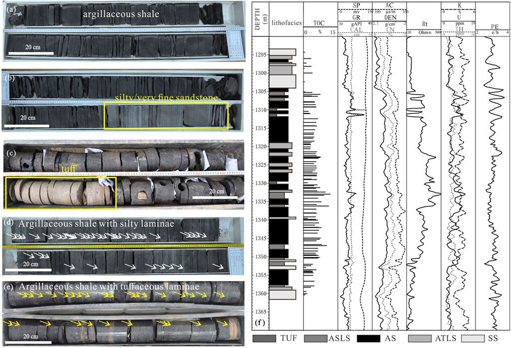
FIGURE 3. The difference of sedimentary and structure on the core scale (A–E): The characteristics of different rock facies on the core (F) distribution and logging response of rock facies in coring section of well YY22.

4.1.2 Distribution characteristics of TOC in lithofacies

In the TOC frequency distribution diagram of different lithofacies shown in Figure 4, there are differences in the distribution range of TOC in different lithofacies. The TOC of TUF and SS is low, mainly distributed below 2.0 wt%, (Figures 4A,B )and the TOC distribution of AS and ASLS is medium (Figures 4C,D). The average values are 5.03 wt% and 6.39 wt% The above four lithofacies have no obvious exhibit skewed distribution with a long tail, and the data have good balance. In the Yanchang Formation shale, the TOC of the ATLS is generally high, and the numerical distribution range is from 3 wt% to 22 wt% (Figure 4E). The frequency distribution guidance diagram of the lithofacies shows a weak skew distribution. Compared with Figure 1C, the proportion of data greater than 8 wt% is all increased, and the imbalance of data is weakened.

FIGURE 4

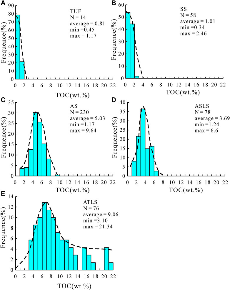
FIGURE 4. Frequency distribution histogram of TOC in TUFF (A), SS (B), AS (C), ASLS (D) and ATLS (E).

The relative proportion of different rock facies in the shale section of the Yanchang Formation is the main reason for the unbalanced distribution of TOC data in Figure 1C. In the shale interval, AS has the highest proportion of thickness, which can account for the total thickness of the shale interval. Secondly, the TOC distribution characteristics of ASLS samples are similar to those of AS, which causes the overall TOC data to be concentrated in the TOC intervals of the above two lithofacies, while in other distribution intervals, especially in the high-value TOC interval of ATLS, there are fewer samples, resulting in unbalanced distribution of data in Figure 1C. The data imbalance of TOC sub-data set of rock facies obtained by classification is reduced, which is helpful for learning algorithm to obtain more accurate prediction model.

4.1.3 Relationship between TOC and logging response in different lithofacies

As mentioned above, the relationship between formation logging response and TOC is affected by other formation parameters, including mineral composition, elemental composition, and organic matter type. Table 2 shows the differences in mineral composition and organic matter types between different rock facies.

TABLE 2

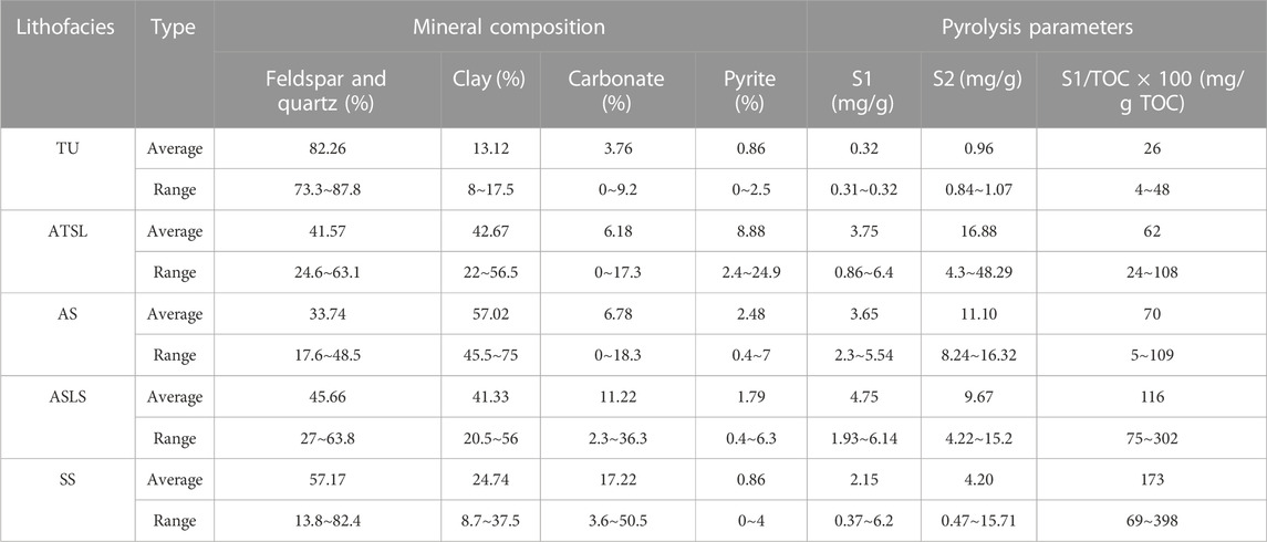
TABLE 2. Comparision of mineral Composition and Pyrolysis parameters for different lithofacies.

From the perspective of mineral composition, AS has the characteristics of high clay mineral content, low felsic content and medium pyrite content. TUF and SS are characterized by low clay mineral content, low pyrite and high felsic content. The difference is that TUF has high carbonate content and SS has high carbonate content. ASLS has obvious transitional characteristics between AS and SS, that is, clay mineral content, carbonate mineral content, clay mineral content and pyrite are all at a medium level; the main characteristic of ATSL is the highest content of pyrite, which can reach 8.9% on average, and other minerals are at a medium level.

Through pyrolysis data, it can be seen that S1 and S2 are higher in the three rock phases of ATSL, AS and ASLE, with an average value of more than 3.5 mg/g and 9.5 mg/g. The S1 and S2 values of SS are lower, with an average value of 2.15 mg/g and 4.2 mg/g. The S1 and S2 values of TUF are the lowest, and S1 and S2 are below 1 mg/g. From the S1/TOC × 100 index, the SS value is the highest, reaching an average of 173 mg/g TOC, followed by ASLS (an average of 116 mg/g TOC), The average value of AS and ATSL is about 65 mg/g TOC, and TU is the lowest, only 26 mg/g TOC. S1/TOC is often used to evaluate the oil content in rocks (Jarvie, 2008). Considering that shale oil may adsorb/dissolve in kerogen, the higher S1/TOC value is generally considered to be a higher content of movable oil, that is, the higher oil content in pores (Li et al., 2015).

In addition, Qiu et al. (2014) and Akhtar et al. (2018) studied the geochemical characteristics of tuff layers in the Yanchang Formation of the Ordos Basin and found that tuff layers generally have high U and Th contents. In a comparative study, Lu (2020) and Yin et al. (2017) found that the layers of siltstone or silty lamina in Zhangjiatan shale often have low U and Th content, while argillaceous shale has relatively high U and Th content.

Figure 5 shows the logging response distribution of each rock facies in different TOC intervals, and the trend line is drawn by the connection of 50th perecentile point in each interval. Because tuff generally has the characteristics of hole enlargement (as shown in Figure 3F, YY22 well 1310 m), the logging response value has great uncertainty, so the relevant data of tuff are not drawn. It can be seen from Figure 5 that there are great differences in the logging response trend lines between different TOC intervals in different rock facies, which also shows that the differences in mineral composition, element composition and oil content of different rock facies will affect the relationship between logging response and TOC.

FIGURE 5

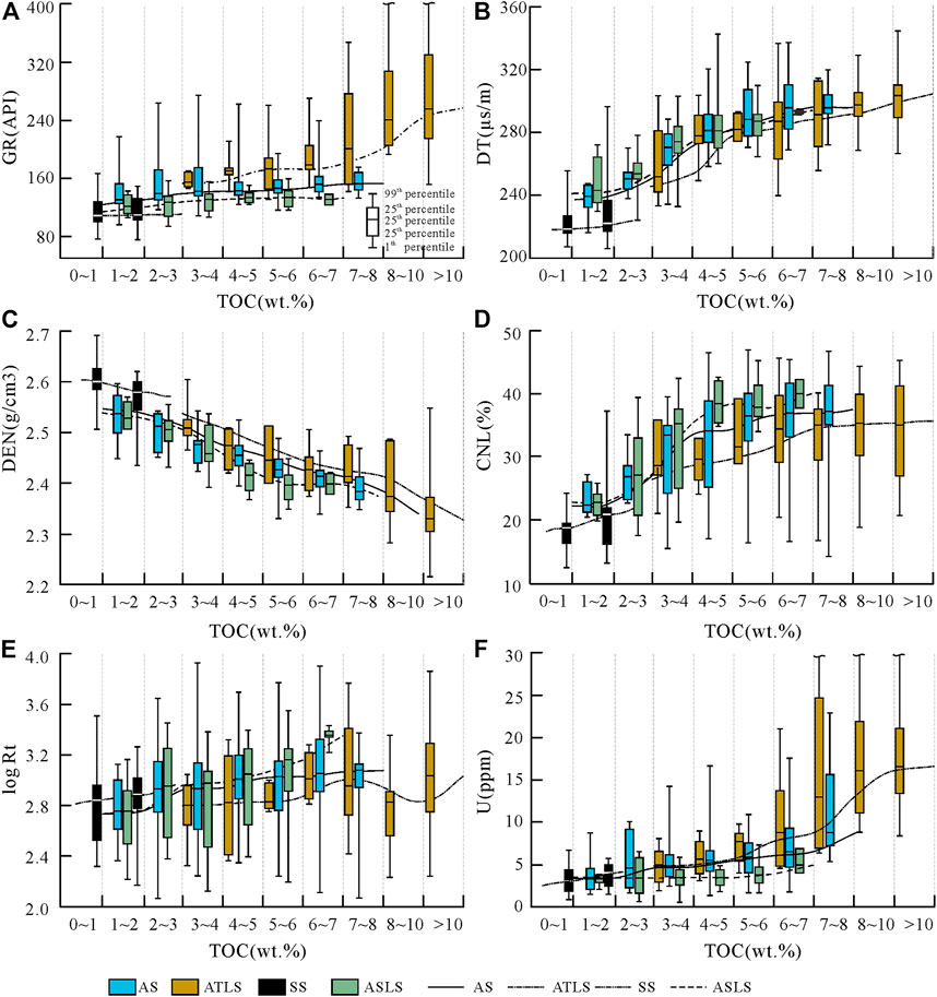
FIGURE 5. Distribution characteristics of GR (A), DT (B), DEN (C), CNL (D), logRt (E), and U (F) in different TOC intervals of rock facies.

From Figure 5, the relationship between TOC and logging response in different lithofacies can be classified into two categories:

One is that the trend lines are similar in direction but not coincident, as shown in Figures 5A–F. In Figures 5A, F, because ATLS has the highest U and Th content, it often has higher GR and U logging values under the same TOC conditions as other lithofacies. Similar SS and ASTL have lower U and Th than AS, which makes it have lower GR and U values. The difference in mineral composition may be the main reason for the inconsistency of the trend lines in Figures 5B, C. For example, the high density of pyrite and carbonate makes ASTL and SS lithofacies have higher density values under the same TOC, and similar minerals also make ASTL and SS have lower acoustic time difference. The difference in oil content caused the non-coincidence of the trend line in Figure 5D. Oil has a higher H+ content than kerogen, resulting in SS and ASLS with higher S1/TOC under the same TOC. Higher neutron porosity values, on the contrary, ASTL neutron porosity is low.

The second is the difference in the direction of the trend line, as shown in Figure 5E, the resistivity logging response distribution in different TOC intervals. The obvious feature is that the trend line of ATLS lithofacies is not obvious, and even in some TOC intervals, the resistivity decreases with the increase of TOC. The high content of pyrite in ATLS may be a key factor in this phenomenon, which also causes the resistivity of ATLS to be generally lower than that of other rock phases under the same TOC. Secondly, the low content of clay minerals with good conductivity and high oil content also lead to higher resistivity of SS and ASLS than AS.

It can be seen that the introduction of rock facies in the analysis of TOC and logging response relationship can better understand the relationship between TOC and different logging responses, so that the relationship is less affected by shale formation factors such as mineral composition and element composition.

4.2 TOC interpretation of LBCRM

4.2.1 Model building

In this study, four SVR models of rock facies were constructed, which were AS, SS, ATLS and ASLS. For three purposes, the prediction model of tuff facies (TUF) was not constructed: 1) the phenomenon of borehole enlargement is obvious in this lithofacies, and the quality of logging data is poor; 2) The proportion of tuff facies in the Yanchang Formation reservoir is low, and the number of TOC test samples is small. 3) The TOC content of the lithofacies is generally low and the values are concentrated (Figure 4A). Datas are derived from FY1, YY18, WY1, YY12, YY2, YY27, YY28, and B36 wells. The total number of data is 412, of which AS, SS, ATLS and ASLS are 214,55,71 and 72 respectively. The above data are randomly assigned to supervised training data sets and validation sets at a ratio of 1:4.

For the need of comparison, this study also constructed a prediction model under the uniform regression fitting mode. The same as the above data, the supervised data did not contain the relevant samples of tuff facies, and the supervised training data set and verification set were obtained from the corresponding data sets of the above four lithofacies. The supervised data include seven kinds of data such as AC, DEN, GR, Rt, PE, Th/K, U/Th, and TOC. The data normalization is carried out by the following formula:

$y_i^{\prime }=\frac{y_{\mathit{max}}-y_i}{y_{\mathit{max}}-y_{\mathit{min}}}.(23)$

Among them, the logging data uses the same maximum and minimum values in the above five supervised data sets. Since the TOC of the samples in SS is much lower than that of the other rock facies, in order to ensure the final prediction accuracy, the TOC of the SS supervised data set is normalized to [0,3], and the TOC of the remaining four supervised data sets is normalized to [0,30], which is normalized to [0,30] in the uniform regression fitting model.

In this study, SVR is used as the basic algorithm, and genetic algorithm is used to optimize the hyper-parameters in SVR. The optimized parameters include kernel function type and its key parameters (Table 3). The fitness function of the genetic algorithm is the cross-validation MSE of the training data (using the K-fold cross-validation method, K = 3). The genetic algorithm uses the bidding model to select the optimal individual (the selection ratio is 0.2). After crossover and mutation operations, a new generation of population is formed. The number of populations in each generation is 150, and the number of iterations is 200. Table 3 shows the range of hyperparameter optimization.

TABLE 3

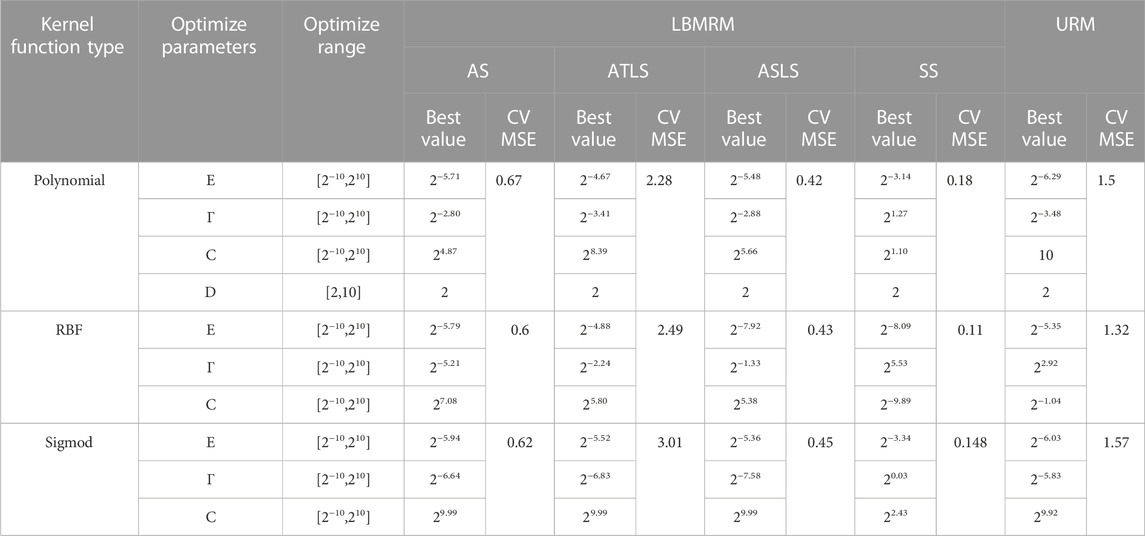
TABLE 3. Optimal parameter series and cross validation root mean square error of SVM regressor obtained by genetic algorithm under different kernel function parameters.

SVR and genetic algorithm are implemented based on libsvm (https://www.csie.ntu.edu.tw/∼cjlin/libsvm/) and geatpy package (http://geatpy.com/index.php/quickstart/).

4.2.2 Performance of model prediction

Figure 6 shows the fitness curves of TOC interpretation model (Figures 6A–D) and homogeneous regression interpretation model (Figure 6E) based on rock facies classification and regression under genetic algorithm optimization. Table 4 lists the optimal parameters of the above optimization process and their corresponding cross validation MSE. It can be found from Figure 6 and Table 4 that the RBF kernel function obtains higher cross-validation accuracy in both interpretation models, that is, the cross-validation MSE is the smallest, which is better than the other two kernel functions. The optimal cross MSE obtained by the RBF kernel function in the homogeneous regression interpretation model is 1.3. In the TOC interpretation model based on rock facies classification regression, the optimal cross MSE in the tuffaceous/clay interbedded shale data set is 2.18, and the optimal root mean square error of other data sets is less than 0.7.

FIGURE 6

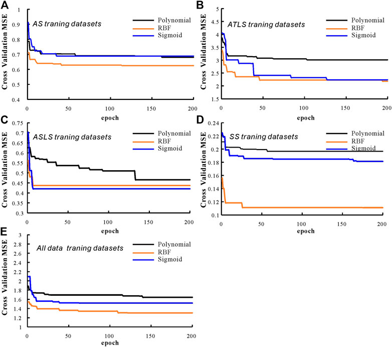
FIGURE 6. Curve of the fitness with the genetic algorithm otimization in AS training datasets (A), ATLS training datasets (B), ASLS training datasets (C), SS training datasets (D) and all data training datasets (E).

TABLE 4

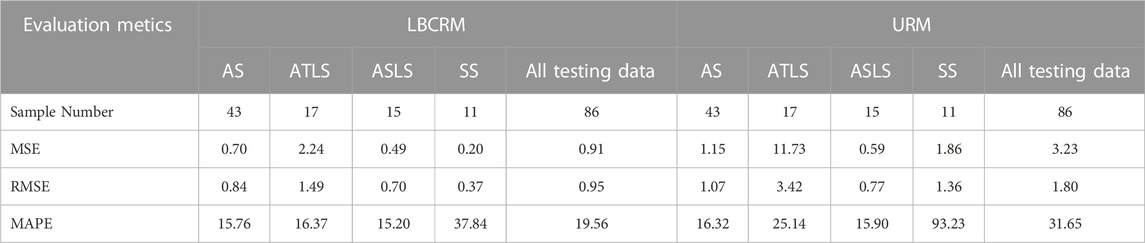
TABLE 4. Interpretation accuracy evaluation indexes of LBCRM and URM applied in different petrographic verification sets.

In order to better evaluate the generalization ability and prediction accuracy of the above model, the above model is applied in the corresponding validation set, and the TOC in each validation set data is predicted respectively. Figure 7 is the projection plot of the predicted TOC value and the measured TOC value of different prediction models. Figure 7A is the projection plot of the prediction results of the uniform regression interpretation model in its response data set, and Figure 7B is the projection plot of the prediction results of the classification regression interpretation model based on lithofacies in their respective validation data sets. Figure 7A shows that the overall prediction effect of the uniform regression interpretation model is poor. As shown in Table 4, MSE is 3.23, RMSE is 1.80, and MAPE is 31.65. It is worth noting that in the interval of TOC>9% in Figure 7A, the predicted value of the prediction model seriously deviates from the true value, and the relative error of the predicted value of individual data points is far more than 25%. In comparison, the classification regression interpretation model based on rock facies shown in Figure 7B has better prediction performance. The distribution of data points is closer to the baseline of real TOC equal to predicted TOC. The MSE, RMSE and MAPE in the evaluation indexes are 0.91, 0.95 and 19.56, respectively. The prediction ability is greatly improved compared with the uniform regression model.

FIGURE 7

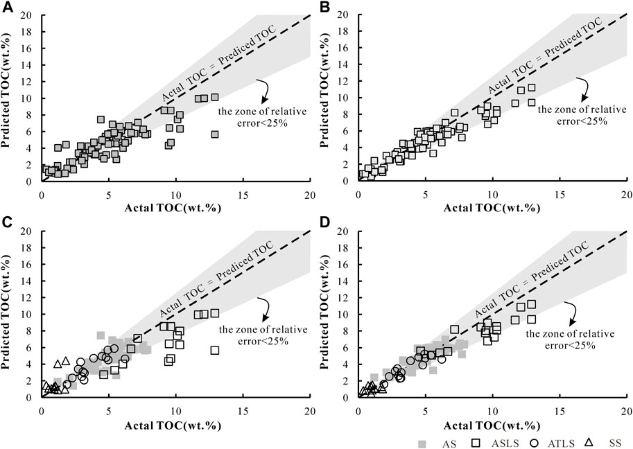
FIGURE 7. Comparison of measured and predicted TOC (A,C): using uniform regression prediction model;(B,D): classification regression prediction model based on rock facies. The different form of data points in Figures (C,D) represent lithofacies types.

Through the difference of prediction performance of the two interpretation models in different rock facies, the reason of poor prediction performance of homogeneous prediction model can be further analyzed. Figure 7C shows the relationship between real and predicted TOC in different lithofacies under the homogeneous regression model. It can be seen from the figure that although the overall prediction performance is not good, the homogeneous regression model has higher prediction performance on AS and ASLS, and each evaluation index is at a lower level. The reason for the great decrease of prediction performance is ATLS and SS. The evaluation indexes MSE, RMSE and MAPE of ATLS prediction results are 11.73, 3.42 and 25.14 respectively. Considering the low TOC characteristics of SS, it may be more appropriate to use MAPE for evaluation, but MAPE = 93.23 is obviously beyond the acceptable range. The reason for the above characteristics can be attributed to the fact that the uniform regression model makes the learning algorithm pay more attention to the learning of data features in the high distribution density interval. The SVR algorithm learns more feature information from the 3% ∼ 8% interval shown in Figure 1C for training, so that the evaluation index MSE is minimized. In this case, the prediction model will extract features from the two lithofacies of AS and ASLS. Figure 5 shows that the characteristics of TOC and logging in different lithofacies have certain differences, which results in the decline of prediction performance in ATLS and SS.

The classification regression prediction model based on lithofacies solves the problem of poor prediction performance of single prediction model in ATLS and SS, making the prediction performance close to AS and ASLS. As shown in Table 4, the prediction indexes of ATLS and SS have been greatly improved (Figure 7D). The MSE, RMSE and MAPE of ASLS are 2.24.1.49 and 16.37 respectively, and SS is 0.20,0.37 and 37.84 respectively. At the same time, the prediction performance of AS and ASLE has also been improved. For example, the MSE, RMSE and MAPE of AS are reduced to 0.70,0.84 and 15.76, and ASLS is reduced to 0.49,0.70 and 15.20, respectively.

The above prediction results show that the classification regression interpretation based on lithofacies can obtain better TOC prediction accuracy in the case of data imbalance and multi-stratigraphic factors.

4.3 TOC computation in shale interval by LBCRM

4.3.1 Model construction and performance evaluation of lithofacies test interpretation

The basis for the application of TOC interpretation model with better prediction performance is lithofacies interpretability. In this study, the lithofacies delineated in the coring section of 8 wells and their corresponding logging response values are used as supervised data sets, and the lithofacies logging recognition model is established by XGBoost algorithm.

The supervised data set includes seven kinds of logging data and lithofacies labels such as AC, DEN, GR, U, CAL, Th and Rt. The logging data uses the original data, and the lithofacies are coded according to TUFof 1, ATLS of 2, AS of 3, ASLS of 4, SS of 5. The XGboost algorithm is based on the XGboost package (https://github.com/d mlc/xgboost). The base model type is gbtree, the learning task is multi: softmax, and the learning objective is mlogloss. In XGboost training, K-fold cross-validation is used to obtain the cross-validation mlogloss value to determine the optimal number of iterations of the tree in XGboost, where K = 7, the maximum number is 200, and the optimal number of iterations is output after 30 iterations without performance improvement. Hyperparameters such as learning rate, max _ depth, min _ child _ weight, gamma and sub _ sample are optimized by genetic algorithm. The fitness function is set to cross mlogloss. The optimization range and coding method are shown in table 5.

TABLE 5

TABLE 5. Parameter to be optimized of XGboost and its optimal value in genetic algorithm.

Figure 8A shows the optimal and average fitness curves in the genetic algorithm optimization process, where the optimal mlogloss is 0.019, and the optimal parameters shown in Table 5 are determined. The maximum number of times obtained by using this parameter is 179. Using the prediction model obtained by this parameter training, 556 data points in the coring sections of WY1 and FY3 were identified, and the confusion matrix shown in Figure 8B was drawn (Figure 8C).

FIGURE 8

FIGURE 8. (A) The fitness change curve of genetic algorithm in XGBoost rock facies logging interpretation model optimization; (B) The confusion matrix of prediction results and measured results in WY1 and FY3 using XGboost rock facies logging interpretation model; (C) Comparison of rock facies prediction results and real results of Well WY1.

The prediction accuracy of the model in the prediction set, the prediction accuracy and recall rate of each class are calculated by the confusion matrix (Table 6). It can be seen that the accuracy and recall rate of the four rock phases of TUF, ATLS, AS and SS are greater than 0.80, and the prediction accuracy and recall rate of ASLS are low, which can still reach about 0.75. The overall prediction accuracy is 0.86, which shows that the prediction model has high prediction accuracy and lays the foundation for the application of LBCRM model in actual drilling.

TABLE 6

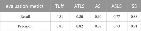
TABLE 6. Evaluation metrics of XGboost classification model in validation set.

4.3.2 Application for TOC content assessment

Based on lithofacies prediction model and LBCRM method, the TOC content of shale can be predicted. Firstly, the lithofacies prediction model is used to identify the lithofacies types of shale section, and the response TOC interpretation model is used to predict TOC for each lithofacies type. Figure 9 shows the lithofacies identification and TOC interpretation results of the shale depth section of 1,250 ∼ 1,340 m in Well FY3. For comparison, the figure also shows the TOC calculated by a single regression model. It can be seen from Figure 9 that the TOC interpretation results obtained by the LBCRM, TOC interpretation model are closer to the measured values. Especially at 1,277 ∼ 1,283 m, LBCRM successfully explained that in addition to the high TOC content in this depth section, the single regression model explained it as lower TOC.

FIGURE 9

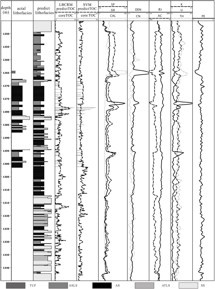
FIGURE 9. The prediction results of lithofacies and TOC in 1,250 ∼ 1,340 m shale section of FY3.

4.4 Inspiration to model - Based interpretation

Model-based TOC interpretation is a method of TOC interpretation under appropriate assumptions and key parameters (Huang and Williamson, 1996; sondergeld et al., 2010). The strong heterogeneity of shale makes it difficult to accurately explain the TOC distribution of shale sections in the application of model-based interpretation methods. The LBCRM interpretation method based on the understanding of shale heterogeneity can better understand the model-based interpretation method and make the latter play a role in the logging interpretation of some key parameters.

ΔlogR is the most classical and widely used model-based TOC interpretation method. Passey et al. (1990) pointed out that in immature shale, the resistivity curve is close to the base value, and ΔlgR is mainly provided by the amplitude of acoustic time difference deviating from the base value. In mature shale, both resistivity and acoustic travel time deviate from the baseline, and ΔlgR comes from the amplitude of the above two deviations from the base value. This also caused a statistically non-linear relationship between TOC, AC, Rt and maturity (Ro).

However, there are obvious differences in the content of conductive minerals and oil content between different rock phases, which will inevitably affect the relationship between ΔlgR-TOC by adding additional factors beyond maturity. For example, the relationship between resistivity and TOC shown in Figure 5E, in the case of the same TOC, the ATLS has the characteristics of low resistivity and low acoustic time difference, and has the characteristics of low maturity in the ΔlogR chart shown in Figure 10A (Passey et al., 1990). The resistivity logging values of SS and ASLS are larger due to high oil content, which makes them have high maturity characteristics in the ΔlogR chart, and the two lithofacies often cross multiple LOM intervals; in the ΔlogR chart, the data points from AS are often concentrated in or near a certain LOM interval. The influence of shale heterogeneity on the Δlog method has prompted a large number of scholars to propose improved models (Wang et al., 2016; zhao et al., 2017), these methods without exception hope to expand the reference range of Δlog by selecting different baselines.

FIGURE 10

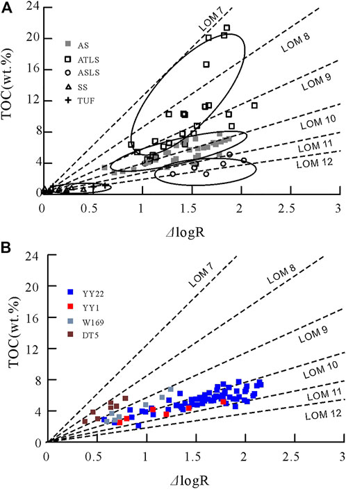
FIGURE 10. (A) The distribution characteristics of different rock facies on the ΔlgR chart; (B) Thermal evolution maturity prediction based on ΔlogR plot using AS ata.

This paper does not focus on improving the traditional model-based prediction method to achieve better TOC prediction performance, but according to the characteristics of AS concentrated in a certain LOM interval in ΔlogR, the combination of LBCRM and ΔlogR is proposed to realize the logging estimation of Ro. Through the data distribution of AS on the ΔlogR-TOC chart of YY22, YY1, W169 and DT5 wells (the data are all derived from the shale of Chang 7) (Figure 10B), the LOM of the above 4 wells is estimated. Based on the conversion relationship between LOM and Ro by Passey (2010), the Ro distribution interval can be estimated (Table 7), Compared with the measured Ro of four wells in this area by Cai et al. (2020), the estimated value is close to the measured value, which fully shows that LBCRM can not only use logging to obtain more accurate TOC distribution in shale section, but also help geologists to explain more formation parameters after being used together with the model-based method.

TABLE 7

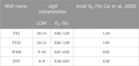
TABLE 7. Comparison of Ro based on AS data and ΔlogR chart interpretation with real Ro.

5 Conclusion

1) In this study, a TOC interpretation model based on lithofacies classification regression was proposed. Through the study of shale heterogeneity characteristics, this method can effectively reduce the influence of formation factors other than TOC on prediction accuracy by constructing TOC interpretation model for each rock facies category, and reduce the degree of data imbalance distribution, so that the data mining algorithm can achieve better prediction results.

2) The interpretability of lithofacies logging ensures the wellsite application based on the regression model of lithofacies classification. Compared with the traditional homogeneous regression model, the prediction performance is greatly improved, and the prediction of high TOC and low TOC sections is more accurate.

3) The LBCRM method based on the heterogeneity of shale can better understand the reasons for the deviation of traditional model-based interpretation methods. When combined with the latter, it can make the logging data provide more useful information.

Data availability statement

The original contributions presented in the study are included in the article/Supplementary Material, further inquiries can be directed to the corresponding author.

Author contributions

JY, CG and MC conceived and designed the experiments; QL, PX and SH performed the experiments; JY and CG analyzed the data; QZ contributed with figures l; JY, CG and MC wrote the paper. All authors read and approved the final manuscript.

Funding

This study was supported by the Major National Science and Technology Projects (No. 2017ZX05039001-005), the Research Project of YanchangOil Field Co., Ltd., 0 (No. ycsy2021jcts-B-06 and ycsy2022jcts-B-28), key R&D plan of Shaanxi Province (No. 2022GY-138,2021GY-113 and S2022-YF-YBGY-0471) and the National Natural Science Foundation of China (No. 41902136).

The authors declare that this study received funding from the Research Project of Yanchang Oil Field Co., Ltd.. The funder was not involved in the study design, collection, analysis, interpretation of data, the writing of this article or the decision to submit it for publication.

Conflict of interest

Authors TJY, CG, SQL, PX, YSH and QZ were employed by Shaanxi Yanchang Petroleum (Group) Corp.Ltd.

The remaining author declare that the research was conducted in the absence of any commercial or financial relationships that could be construed as a potential conflict of interest.

Publisher’s note

All claims expressed in this article are solely those of the authors and do not necessarily represent those of their affiliated organizations, or those of the publisher, the editors and the reviewers. Any product that may be evaluated in this article, or claim that may be made by its manufacturer, is not guaranteed or endorsed by the publisher.

References

Akhtar, S., Sahir, N., and Yang, X. Y. (2018). Genesis of tuff interval and its uranium enrichment in upper triassic of ordos Basin, NW China. Acta Geochim. 37, 32–46.

CrossRef Full Text | Google Scholar

Aldrich, J., and Seidle, J. (2018). “Sweet spot” identifcation and optimization in unconventional reservoirs,” in AAPG datapages/search and discovery article #90323 (Salt Lake City, Utah.

Google Scholar

Alfred, D., and Vernik, L. (2012). “A new petrophysical model for organic shales,” in SPWLA 53rd annual logging symposium (Colombia: Cartagena).

Google Scholar

Altowairqi, Y., Rezaee, R., Evans, B., and Urosevic, M. (2015). Shale elastic property relationships as a function of total organic carbon content using synthetic samples. J. Pet. Sci. Eng. 133, 392–400. doi:10.1016/j.petrol.2015.06.028

CrossRef Full Text | Google Scholar

Branco, P., Torgo, L., and Ribeiro, R. P. (2018). Rebagg: Resampled BAGGing for imbalanced regression. Proceeedings Mach. Learn. Res. 94, 1–15.

Google Scholar

Branco, P., Torgo, Luís, and Ribeiro, R. P. (2016). A survey of predictive modeling on imbalanced domains. ACM Comput. Surv. (CSUR) 49 (2), 1–50. doi:10.1145/2907070

CrossRef Full Text | Google Scholar

Buda, M., Maki, A., and Mazurowski, M. A. (2018). A systematic study of the class imbalance problem in convolutional neural networks. Neural Netw. 106, 249–259. doi:10.1016/j.neunet.2018.07.011

PubMed Abstract | CrossRef Full Text | Google Scholar

Cai, Z. J., Lei, Y. H., Luo, X. R., Wang, X. Z., and Cheng, M. (2020). Characteristics and controlling factors of organic pores in the 7th member of Yanchang Formation shale in the Southeastern Ordos Basin (in Chinese). Oil& Gas. Geol. 41 (2), 367–379.

Google Scholar

Carpentier, B., Huc, A. Y., and Bessereau, G. (1991). Wireline logging and source rocks estimation of organic carbon by the Carbolog method. Log. Anal. 32 (3), 279–297.

Google Scholar

Chan, S. A., Hassan, A. M., Usman, M., Humphrey, J. D., Alzayer, Y., and Duque, F. (2022). Total organic carbon (TOC) quantification using artificial neural networks: Improved prediction by leveraging XRF data. J. Pet.sci.eng. 108, 109302. doi:10.1016/j.petrol.2021.109302

CrossRef Full Text | Google Scholar

Chen, T. Q., and Guestrin, C. “XGBoost: A scalable tree boosting system,” in 22nd ACM SIGKDD International Conference on Knowledge Discovery and Data Mining, New York, NY, USA, 2016, 785–794.

Google Scholar

Chen, Y. Y., Gao, D. C., and Sun, X. N. (2020). Organic Geochemistry and Evaluation of the Shale of Yanchang Formation in Yanchang Exploration Area of Ordos Basin. Unconv. Oil Gas 7 (1), 32–37. doi:10.3969/j.issn.2095-8471.2020.01.007

CrossRef Full Text | Google Scholar

Curtis, J. B. (2002). Fractured shale-gas systems. Am. Assoc. Pet. Geol. Bull. 86, 1921–1938.

CrossRef Full Text | Google Scholar

Dellenbach, J., Espitalie, J., and Lebreton, F. (1983). “Source rock logging,” in Transactions of the SPWLA 8th European formation evaluation symposium (London, UK).

Google Scholar

Gao, F., Song, Y., Li, Z., Xiong, F., Chen, L., Zhang, Y., et al. (2018). Lithofacies and reservoir characteristics of the Lower Cretaceous continental Shahezi Shale in the Changling Fault Depression of Songliao Basin, NE China. Mar. Petroleum Geol. 98, 401–421. doi:10.1016/j.marpetgeo.2018.08.035

CrossRef Full Text | Google Scholar

Guo, S. B., Wang, Z. L., and Ma, X. (2021). Exploration prospect of shale gas with Permian transitional facies of some key areas in China. Pet. Geol. &Experiment 43 (3), 377–385. doi:10.11781/sysydz202103377

CrossRef Full Text | Google Scholar

Holland, J. (1973). Erratum: genetic algorithms and the optimal allocation of trials. SIAM J. Comput. 2 (2), 88–105. doi:10.1137/0202009

CrossRef Full Text | Google Scholar

Huang, Z. H., and Williamson, M. A. (1996). Artificial neural network modelling as an aid to source rock characterization. Mar. Petroleum Geol. 13 (2), 277–290. doi:10.1016/0264-8172(95)00062-3

CrossRef Full Text | Google Scholar

Jarvie, D. M. (2008). Unconventional shale resource plays: Shale-gas and shale-oil opportunities. New York, NY, USA: Fort Worth Business Press Meeting.

Google Scholar

Li, J. J., Wang, W. M., Cao, Q., Shi, Y. L., Yan, X. T., and Tian, S. S. (2015). Impact of hydrocarbon expulsion efficiency of continental shale upon shale oil accumulations in eastern China. Mar. Petroleum Geol. 59, 467–479. doi:10.1016/j.marpetgeo.2014.10.002

CrossRef Full Text | Google Scholar

Liang, X. W., and Li, L. (2021). Geological conditions and exploration potential for shale gas in Upper Permian Wujiaping Formation in the region of Western Hubei-eastern Chongqing[J]. Pet. Geol. &Experiment 43 (3), 386–394. doi:10.11781/sysydz202103386

CrossRef Full Text | Google Scholar

Liu, Z., Miao, Z., Zhan, X., Wang, J., Gong, B., and Yu, S. X. (2019). Large-scale long-tailed recognition in an open world. louisiana, LA, USA: CVPR.

Google Scholar

Long, H. C., and Li, S. P. (2022). The research on the heterogeneity of shale formations and its controlling factors—A case study of the second member of Funing Formation in Subei Basin[J]. Unconv. Oil Gas 9 (04), 78–90.

Google Scholar

Lu, H. (2020). Master's Thesis. Beijing, China: China university of petroleum Beijing, 141.Study on tuff reservoir characteristics and formation mechanism of the Chang 7 member in the southern Ordos Basin,

Google Scholar

Ma, Y. Z. (2015). “Unconventional resources from exploration to production,” in Unconventional oil and gas resources handbook: Evaluation and development (Netherlands, Europe: Elsevier), 3–52.

Google Scholar

Mahmoud, A., Elkatatny, S., Mahmoud, M., Abouelresh, M., Abdulraheem, A., and Ali, A. (2017). Determination of the total organic carbon (TOC) based on conventional well logs using artificial neural network. Int. J. Coal Geol. 179, 72–80. doi:10.1016/j.coal.2017.05.012

CrossRef Full Text | Google Scholar

Meng, Q. Q., Li, J. Z., Liu, W. H., Fu, Q., Wang, X. F., and Wang, J. (2022). Simulation Study on the Effect of Gypsum-salt Content on Hydrocarbon Generation in Mature Stage Shale. Special Oil Gas Reservoirs 5, 113–118.

Google Scholar

Meng, Q. Q. (2022). Identification method for the origin of natural hydrogen gas in geological bodies[J]. PETROLEUM Geol. Exp. 44 (3), 552–558. doi:10.11781/sysydz202203552

CrossRef Full Text | Google Scholar

Ou, C. H., Li, C. C., Rui, Z. H., and Ma, Q. (2018). Lithofacies distribution and gas-controlling characteristics of the Wufeng–Longmaxi black shales in the southeastern region of the Sichuan Basin, China. J. Petroleum Sci. Eng. 165, 269–283. doi:10.1016/j.petrol.2018.02.024

CrossRef Full Text | Google Scholar

Passey, Q. R., Bohacs, K., Esch, W. L., Klimentidis, R., and Sinha, S. (2010). “From oil-prone source rock to gas-producing shale reservoir-geologic and petrophysical characterization of unconventional shale gas reservoirs,” in International oil and gas conference and exhibition in China (London, UK: Society of Petroleum Engineers).

CrossRef Full Text | Google Scholar

Passey, Q. R., Creaney, S., Kulla, J. B., Moretti, F. J., and Stroud, J. D. (1990). A practical model for organic richness from porosity and resistivity logs. AAPG Bull. 74 (12), 1777–1794.

Google Scholar

Qiu, X. W., Liu, C. Y., Mao, G. Z., Deng, Y., Wang, F. F., and Wang, J. Q. (2014). Late Triassic tuff intervals in the Ordos basin, Central China: Their depositional, petrographic, geochemical characteristics and regional implications. J. Asian Earth Sci. 80, 148–160. doi:10.1016/j.jseaes.2013.11.004

CrossRef Full Text | Google Scholar

Schlanser, K. M. (2015). Lithofacies classification in the Marcellus Shale and surrounding formations by applying Expectation Maximization to petrophysical and elastic well logs. Laramie, WY, USA: University of Wyoming.

Google Scholar

Schmoker, J. W. (1979). Determination of organic content of Appalachian Devonian shale from formation-density logs. AAPG Bull. 63 (9), 1504–1509.

CrossRef Full Text | Google Scholar

Schmoker, J. W. (1981). Determination of organic matter content of Appalachian Devonian shale from gamma-ray logs. AAPG Bull. 65 (7), 1285–1298.

CrossRef Full Text | Google Scholar

Singh, P. (2008). Lithofacies and sequence stratigraphic framework of the barnett shale, northeastern Texas. Ph.D. Dissertation. Norman, Oklahoma: University of Oklahoma, 81.

Sondergeld, C. H., Newsham, K. E., Comisky, J. T., Rice, M. C., and Rai, C. S. (2010). “Petrophysical considerations in evaluating and producing shale gas resources,” in SPE unconventional gas conference (Pennsylvania, PA, USA: Society of Petroleum Engineers).

CrossRef Full Text | Google Scholar

Tan, M., Song, X., Yang, X., and Wu, Q. (2015). Support-vector-regression machine technology for total organic carbon content prediction from wireline logs in organic shale: a comparative study. J. Nat. Gas. Sci. Eng. 26 (1), 792–802. doi:10.1016/j.jngse.2015.07.008

CrossRef Full Text | Google Scholar

Vapnik, V. N. (1995). The nature of statistical learning theory. New York, NY, USA: Springer-Verlag, 188.

Google Scholar

Wang, G. C., Carr, T. R., and Ju, Y. W. (2014). “Statistical reverse model to predict mineral composition and TOC content of Marcellus shale”, in SPE Unconventional Resources Conference. Woodlands, TX, United States: Society of petroleum Engineers.

CrossRef Full Text | Google Scholar

Wang, G. C., and Carr, T. R. (2012). Methodology of organic-rich shale lithofacies identification and prediction: A case study from Marcellus Shale in the Appalachian basin. Comput. Geosciences 49, 151–163. doi:10.1016/j.cageo.2012.07.011

CrossRef Full Text | Google Scholar

Wang, H., Wu, W., Chen, T., Dong, X., and Wang, G. (2019). An improved neural network for TOC, S1 and S2 estimation based on conventional well logs. J. Pet. Sci. Eng. 176, 664–678. doi:10.1016/j.petrol.2019.01.096

CrossRef Full Text | Google Scholar

Wang, P., Chen, Z., Pang, X., Hu, K., Sun, M., and Chen, X. (2016). Revised models for determining TOC in shale play: example from devonian Duvernay shale, Western Canada Sedimentary Basin. Mar. Pet. Geol. 70, 304–319. doi:10.1016/j.marpetgeo.2015.11.023

CrossRef Full Text | Google Scholar

Wei, S. L., Huang, X. B., Li, J., Su, Y. H., and Pan, L. S. (2021). Shale gas EUR estimation based on a probability method:a case study of infill wells in Jiaoshiba shale gas field[J]. Pet. Geol. &Experiment 43 (1), 161–168. doi:10.11781/sysydz202101161

CrossRef Full Text | Google Scholar

Yin, J. T., Yu, Y. X., Jiang, C. F., Liu, J., Zhao, Q. P., and Shi, P. (2017). Relationship between element geochemical characteristic and organic matter enrichment in Zhangjiatan Shale of Yanchang Formation,Ordos Basin. J. China Coal Soc. 42 (6), 1544–1556.

Google Scholar

Yu, H., Rezaee, R., Wang, Z., Han, T., Zhang, Y., Arif, M., et al. (2017a). A new method for TOC estimation in tight shale gas reservoirs. Int. J. Coal Geol. 179, 269–277. doi:10.1016/j.coal.2017.06.011

CrossRef Full Text | Google Scholar

Yu, Y. X., Luo, X. R., Cheng, M., Lei, Y. H., Wang, X. Z., Zhang, L. X., et al. (2017b). Study on the distribution of extractable organic matter in pores of lacustrine shale: an example of zhangjiatan shale from the upper triassic yanchang formation, ordos basin, China. Interpretation 5 (2), 109–126. doi:10.1190/int-2016-0124.1

CrossRef Full Text | Google Scholar

Zhang, Y. Y., Zhao, D. F., Guo, Y. H., Wei, Y., Kang, W. Q., Jiao, W. W., et al. (2022). Systematic classification and characterization of small-scale sedimentary structure of the Wufeng Formation shale based on lithofacies——Influence for the evaluation of deep shale reservoirs[J]. Unconv. Oil Gas 9 (02), 26–33.

Google Scholar

Zhao, D. F., Guo, Y. H., Zhu, Y. M., Zhao, S. X., Chen, Z. H., Jiao, W. W., et al. (2022). Comments on the evaluation system of accurate evaluation and selection of deep marine shale reservoirs. Unconv. Oil Gas 9 (02), 1–7.

Google Scholar

Zhao, P. Q., Ma, H. L., Rasouli, V., Liu, W. H., Cai, J. C., and Huang, Z. H. (2017). An improved model for estimating the TOC in shale formations. Mar. Pet. Geol. 83, 174–183. doi:10.1016/j.marpetgeo.2017.03.018

CrossRef Full Text | Google Scholar

Zhen, Q., Tao, Caineng Zou, Wang, Hongyan, Ji, Hongjie, and Zhou, Shixin (2016). Lithofacies and organic geochemistry of the middle permian lucaogou Formation in the jimusar sag of the junggar basin. NW China.

Google Scholar

Zheng, D. Y., Wu, S. X., and Hou, M. C. (2021). Fully connected deep network: An improved method to predict TOC of shale reservoirs from well logs. Mar. Pet. Geol. 132, 105205. doi:10.1016/j.marpetgeo.2021.105205

CrossRef Full Text | Google Scholar

Zhu, L. Q., Zhang, C., Zhang, C. M., Zhang, Z. S., Zhou, X. Q., Liu, W. N., et al. (2020). A new and reliable dual model- and data-driven TOC prediction concept: A TOC logging evaluation method using multiple overlapping methods integrated with semi-supervised deep learning. J. Pet.sci.eng. 188, 106944. doi:10.1016/j.petrol.2020.106944

CrossRef Full Text | Google Scholar