Water level fluctuation controls carbon emission fluxes in a shallow lake in China

High-strength alterations in the water level due to extreme climate change and increased anthropogenic activities have implications for methane (CH₄) and carbon dioxide (CO₂) emission variations in shallow lakes. However, the consistency of the carbon emission flux in response to water-level fluctuations and temperature is still unclear. Here, we evaluated the water depth (WD) on the magnitude and variation sensitivity of CH₄, CO₂, and GHG, and then the temperature dependence of carbon emissions was estimated at different water levels. The water depth threshold indicated a maximum CH₄ (97.5 cm) and CO₂ (10 cm), resulting in a water depth threshold of GHG at 54.6 cm. Inside the whole WD, the effect of rising water depth on CH₄, CO₂ and GHG sensitivity shifted from a positive effect to a negative effect at a WD of 97.5 cm. And CH₄, CO₂ and GHG in 10 cm<WD<97.5 cm show the highest emission flux and sensitivity to varying water depths. Furthermore, a consistency of carbon emission flux responding to water depth and temperature was only found in specific zones of shallow lakes with 10 cm<WD<97.5 cm, indicating that the temperature dependence of CH₄ and CO₂ are driven by the hydrological regime without water level stress, shifting the GHG emission flux. Ensuring the restoration management goal related to the carbon peak by governing the time of threshold occurrence is essential.

1 Introduction

Hydrological regimes of shallow lake wetlands play a vital role in controlling physiochemical, biological processes and function (Poff et al., 1997; Mitsch and Gosselink, 2015; Hilt et al., 2017; Palmer and Ruhi, 2019), especially in the establishment and maintenance of specific wetland types (Mitsch and Gosselink, 2015; Yang et al., 2020). However, strong alterations in hydrological regimes caused by both extreme climate change and increased anthropogenic activities contribute to the widespread loss and degradation of wetlands globally (Millennium Ecosystem Assessment, 2005; Davidson, 2014; Gardner et al., 2015; Liu et al., 2020a). In the restoration process with water regulation (Jiang et al., 2016; Kong et al., 2017; Moor et al., 2017), the abrupt increase in water level elevation due to ecological water transfer projects and reductions in seasonal water level fluctuations resulting from water level controls inevitably induced changes in biological processes while also influencing carbon C) balances (Martínez-Santos et al., 2008; Kong et al., 2017; Olefeldt et al., 2017).

As indicators of C balances, CH₄ and CO₂ fluxes are outputs of biological processes related to moisture restriction, and a threshold is proposed while CH₄ or CO₂ emissions vary with water level according to Shelford’s tolerance law (Shelford, 1913; Shelford, 1931; Odum, 1971; Erofeeva, 2021). Additionally, the threshold is amplified or minimized due to the fluctuating pattern of the water level (e.g., constant non-fluctuation, natural fluctuations driven by normal meteorological factors, and high-strength alterations due to extreme climate change and increased anthropogenic activities) with the same annual or multiyear mean water level.

Shifts in water level lead to threshold variations in CH₄ and CO₂ and are mainly governed by the transfer between anaerobic methane (CH₄) production and aerobic CH₄ oxidation processes. Within the optimal threshold range, higher water levels are generally associated with higher net CH₄ emissions and less CO₂ emissions (Jacinthe, 2015; Li X. et al., 2019; Ye et al., 2019), resulting in uncertainty in total carbon emissions (GHG). The “enzyme latch” theory has been used to clarify wetland C responses to varying water levels (Ise et al., 2008). As shown in a previous study, the reduction of electron acceptor concentrations with water level drawdown alters the accumulation of aromatic solubility and hydrolase activity (Wang et al., 2017), which explains the positive, neutral and negative effects of water level reduction on soil organic carbon (SOC). Additionally, water level fluctuations will alter redox conditions directly, subsequently triggering CH₄ and carbon dioxide (CO₂) emissions to occur (Granberg et al., 1997; Chimner et al., 2016; Van der Lee et al., 2017) and resulting in relative contribution differences to GHGs.

However, the relative contribution difference of CH₄ and CO₂ to GHG threshold uncertainty is larger under multiple stressors. Stressor impacts can combine additively or can interact, causing synergistic or antagonistic effects (Simmons et al., 2021). Birk et al. (2020) evaluated the effects in European lakes, and only one of the two stressors had a significant effect of 39%; 28% of the paired-stressor combinations resulted in additive effects, and 33% resulted in interactive effects. Based on metabolic theory, the temperature dependence of carbon emissions is extremely general in wetlands, including shallow lakes. Studies have shown that both CH₄ and CO₂ show exponential growth within −25°C–35°C (Song et al., 2010; Chen et al., 2021), and temperature dependence is widely found in various wetland types and scales (Yvon-Durocher et al., 2012; Yvon-Durocher et al., 2014; Chen et al., 2021). However, it is unknown whether the GHG threshold uncertainty is amplified or minimized when high-strength water level fluctuations and temperatures act simultaneously.

As the relative contribution variation of CH₄ and CO₂ depends on the anerobic condition change along with water depth (Van der Lee et al., 2017), the threshold of GHG emissions in shallow lakes is between the thresholds of CH₄ and CO₂. Additionally, upon Shelford’s tolerance law and metabolic theory, the sensitivity of carbon emissions to varying water depths is related to temperature. Consequently, the objectives of the present study are 1) to explore the response of the characteristics of CH₄, CO₂ and GHG emissions to water depth; 2) to assess the sensitivity of CH₄, CO₂ and GHG emissions to varying water depths inside or between WD intervals; and 3) to attribute the effects of water depth changes on the temperature dependence of carbon emissions. To achieve this, we subdivided water level intervals based on turning points found in the response process of CH₄ and CO₂ to water depth. Additionally, accounting for the ecological response of CO₂ and CH₄ flux and sensitivity to variations in water depth, we also attempted to extend our results to enrich the general theory as it pertains to shallow lake wetland restoration. In this study, we choose Lake Baiyangdian (BYD) as a case study, using CH₄, CO₂ and GHG as quantitative indicators of carbon emission magnitude and variation.

2 Materials and methods

2.1 Case study

The BYD (38◦43′to 39◦02′N, 115◦38′to 116◦07′E) is the largest inland freshwater lake-marsh wetland in the North China Plain (Figure 1). It includes 94 km² of raised fields and greater than 3700 of ditches that subdivide the basin into 140 small shallow lakes, with a surface area of 366 km² and an average water depth of 2 ± 0.35 m (CCLCAC, 2000). Historically, nine rivers fed the BYD; however, most of these rivers have dried up due to climate changes and increased anthropogenic activities (Liu et al., 2010). Ecosystem processes and functions in the BYD, which is a typical shallow lake for which reeds are the dominant emergent plant, are sensitive to water-level fluctuations, namely, fluctuations related to net primary productivity and organic matter. With a decline in water level, macrophytes, especially reeds, have exhibited a tendency to expand, resulting in terrestrialization in some shallow lakes within the BYD (e.g., Zaozha Lake and Guding Lake) (Cui et al., 2017). To maintain the water ecology and integrity of the BYD, ecological water transfer projects have been implemented since the 1980s to replenish the lake (Wang et al., 2018). Specifically, the planning outline of the Xiong’an New Area, which has jurisdiction over BYD, includes an ordinance for its ecological restoration. Inevitably, under highly intensive anthropogenic activities, hydrological regime alterations have caused aquatic ecosystem changes to occur (Wang et al., 2018; Li Y. L. et al., 2019) and affected the C sequestration capacity of the lake (Li et al., 2009; Chen et al., 2017).

FIGURE 1

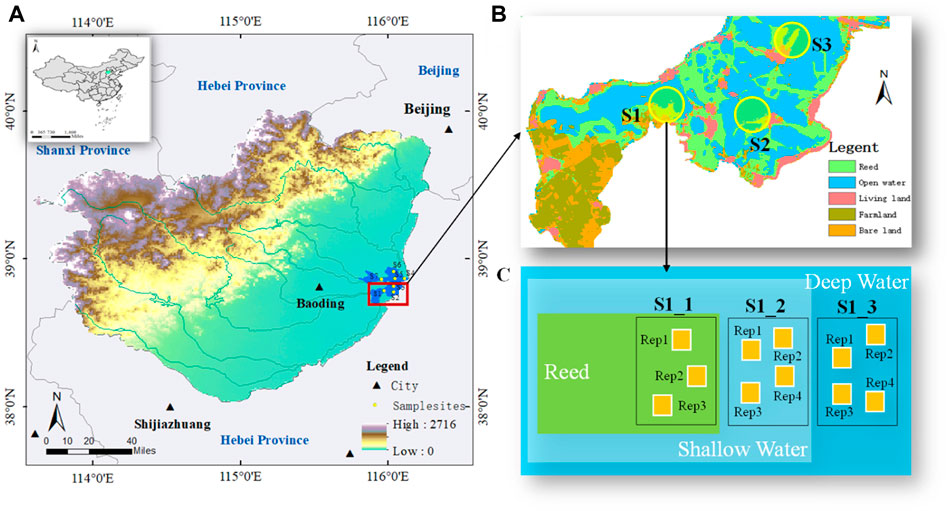
FIGURE 1. Location of Lake Baiyangdian (BYD, Figure 1A), seven sampling strips (Figure 1A; Figure 1B), and repetitions at each sample site (Figure 1C). As shown in Figure 1B, three sample sites were conducted in each sampling strip, where sampling strip S1 is consist of sample sites marked as S1_1, S1_2, and S1_3. And Rep1 to Rep4 showed the repetitions in each sample sites.

Based on our preliminary field investigations, combined with diverse geomorphological, hydrological, and vegetative conditions in the lake, we chose seven sample strips consisting of 21 sample sites (Figure 1A). According to the historical water levels from 1960 to 2019 (Supplementary Figure S1), 21 sample sites were examined considering the annual water depth. As shown in Figures 1B, C, three sample sites were conducted in each sampling strip, where sampling strip S1 consists of sample sites marked as S1_1, S1_2, and S1_3. Triplicates or four repetitions were set for sample sites with water depths of negative and positive, respectively, according to the spatial heterogeneity of terrain and biological factors (Figure 1C). We performed five field surveys: in June, October, and December 2020, and in February and April 2021. We simultaneously tested the water depth (WD) and temperatures of water (T_Water), air (T_Air) and chamber (T_cham) for each field survey. In above, we obtained 105 couples of data for further analysis. And the water depth involved in all sampling sites ranged from -1.10 m to 4.20 m.

2.2 Greenhouse gas and environmental factor measurements

2.2.1 Greenhouse gas collection and measurement

The in situ CH₄ and CO₂ emissions were measured with the static opaque chamber and gas chromatography technique (Zhang et al., 2020; Gao et al., 2022). The fluxes of CH₄ and CO₂ were measured simultaneously with the collection of surface water and local ambient air samples. At each site, four floating chambers were deployed from the open water alongside the zone of emergent vegetation. These chambers were of the same size and shape and streamlined with a flexible plastic foil collar to minimize the effects of chamber-induced turbulence when measuring fluxes. Each chamber was also covered with aluminum foil to reflect sunlight and minimize internal heating. Chambers were allowed to drift, and each chamber measurement lasted for 60–80 min. After mixing the contents of the chambers three times, 50 mL of gas was extracted from the chambers and transferred to airtight gas sampling bags at 0, 5, 10, 20, 40, 60, and 80 min. This multi-chamber method and prolonged deployment not only increased the probability of capturing ebullition but also incorporated spatiotemporal variability in both diffusion and ebullition within and among streams and rivers. The concentrations of CH₄ and CO₂ in the gas samples were determined as described above, and CH₄ and CO₂ fluxes were calculated based on the closed-chamber technique (Yuan et al., 2021).

2.2.2 Meteorological and soil physiochemical property measurements

The water depth, air temperature, temperature in the chamber, and soil temperature at a depth of 5 cm were simultaneously measured in situ while gas samples were collected. For samples in deep water and shallow water, a portable water quality analyzer (Hach H40 d) was used to simultaneously monitor water temperature, pH, dissolved oxygen (DO), and redox potential (Eh).

2.3 Evaluation of carbon emission flux in response to water depth

2.3.1 Assessment of the water depth threshold by a piecewise regression model

As the carbon emission fluxes showed significant piecewise regression varying with water depth, a piecewise regression model was applied to the carbon emission flux series to detect the turning points for CH₄ flux, CO₂ flux and GHG varying with water depth (Toms and Lesperanc, 2003; Yang et al., 2017):

$y=\left\{\begin{array}{cc}{\beta }_0+{\beta }_{1}t+\epsilon & t\le \alpha \\ {\beta }_0+{\beta }_{1}t+{\beta }_2\left(t-\alpha \right)+\epsilon & t>\alpha \end{array}\right\}(1)$

where t is the water depth; y is the carbon emission flux; β₀, β₁ and β₂ are regression coefficients; and α is the assumed turning point, which was determined based on carbon emission flux analysis. The range of the α value was set to be the water depth when β₁ and β₂ were found to be different. Least squares linear regression was used to estimate the three regression coefficients, and a t-test was applied to test if β₂ was not equal to zero.

2.3.2 Sensitivity of carbon emission flux to water depth

To evaluate the sensitivity and final effect of water depth on CH₄, CO₂ and GHG sensitivity, we compare the magnitude of emission sensitivity in all WD intervals with a baseline of average water depth of all sites. The carbon emission flux sensitivity to water depth (ΔC, WD) is equal to the difference between the CH₄, CO₂ and GHG emission fluxes at specific water depths and the average water depth. ΔC, WD is quantified as follows:

$∆\mathrm{C},\mathrm{W}\mathrm{D}=\frac{\left({C_i-C}_0\right)/C_0}{\left({h_i-h}_0\right)/h_0}(2)$

where $∆\mathrm{C},\mathrm{W}\mathrm{D}$ represents the sensitivity of carbon flux equivalent to water depth change (mg CO₂-eq/m²/h/cm), C_i and h_i represent the CH₄ or CO₂ flux in each pair of data points of site i (mg CO₂-eq/m²/h) and the corresponding water depth (cm), and C₀ represents the CO₂ equivalent (mg CO₂-eq/m²/h) corresponding to the average water depth h₀ in the water depth interval of interest. To evaluate the sensitivity of the total carbon emissions GHG at each sampling point, CH₄ flux is converted to CO₂ flux equivalent, and the conversion factor is 25 (Huang et al., 2021).

$\mathrm{G}\mathrm{H}\mathrm{G}=25*{CH}_4+{CO}_2(3)$

2.4 Dependence of carbon emission flux on temperature

To exclude the independence between water depth and temperature, we tested the correlation between each pair of variables. The correlation between temperature and water depth in all WD intervals is identified, and pairs of data with significant correlations are removed. The apparent activation energy was selected as the characterization index of the temperature dependence of carbon emission. The temperature-dependent quantification of CH₄ and CO₂ emissions is based on the Boltzmann-Arrhenius function of the form (Jaap van der Meer, 2006; Price et al., 2010; Chen et al., 2021):

$\mathit{ln}{R}_i\left(T\right)=\left(\overline{E}+{\epsilon }_E^i\right)\left(\frac{1}{{kT}_C}-\frac{1}{kT}\right)+\overline{lnR\left(T_C\right)}+{\epsilon }_R^i(4)$

where lnR_i(T) represents the natural logarithm of the CH₄ or CO₂ emission flux at any location i at the absolute temperature T (K); $\overline{E}$ is the average apparent activation energy (E) between the sample sites, which characterizes the wetland greenhouse temperature dependence of gas emissions; k is the Boltzmann constant (8.62 × 10^–5 eV k⁻¹); and lnR (T_C) represents the natural pair of emission fluxes at the sample site at the T_C level (average temperature in the dataset) number. Consideration of E and emission flux due to differences in other organisms (e.g., substrate supply, microbial community structure and/or composition, physiological adaptation and/or adaptation) and abiotic (e.g., annual mean temperature) between different sites lnR (T_C) estimates were different, and a linear mixed model was used to quantify the temperature dependence of carbon emissions.

2.5 Statistical analysis

The spatiotemporal differences in CH₄ and CO₂ emission fluxes and their significance were characterized using analysis of variance (ANOVA). All variables were tested for homogeneity of variance and normal distribution. For the variable data satisfying the normal distribution, the Pearson correlation coefficient was used for analysis; otherwise, the Spearman correlation coefficient was used for correlation analysis. SPSS 22.0 was used to construct a linear mixed model and quantify the temperature dependence. Then, the slope and intercept are treated as random variables according to the mean of $\overline{E}$; $\overline{lnR\left(T_C\right)}$, and the sample point deviation is defined as the average value of each sample ${\epsilon }_E^i$; ${\epsilon }_R^i$, respectively, so that the sample difference is related to carbon. The magnitude of the overall effect of the emission temperature dependence was quantified as the standard deviation of the random effects term. In terms of random effect model selection for data analysis in different water depth intervals, SPSS 22.0 is used to evaluate different models, and the Akaike information criterion (AIC) in the maximum likelihood method is used to evaluate whether different random variables are included in the linear mixed model. The selection of random variable parameters is performed. The smaller the AIC value is, the better the effect. Among them, Model one includes all potential fixed effects and only one random effect, corresponding to the change in intercept, and Model two includes all potential fixed effects and two random effects, that is, corresponding to the change in slope and intercept.

3 Results

3.1 Carbon emission flux varying with water depth

The CH₄, CO₂ and GHG fluxes varied with water depth, and turning points were found at 97.5 cm, 10 cm and 54.6 cm (water depth threshold, WDT), respectively. As shown in Figure 2, CH₄ and CO₂ fluxes increased when the water depth was less than the WDT, while decreasing trends were shown when the water depth was larger than the WDT. CH₄ flux and CO₂ flux ranged from −0.07 mg CO₂-eq/m²/h to 8.32 mg CO₂-eq/m²/h and −4.76 mg CO₂/m²/h to 196.52 mg CO₂/m²/h, respectively, with a higher absolute value of the regression slope at water depths of -97.5 cm–54.6 cm. The regression slopes of CH₄ and CO₂ are 0.018 and −0.008 mg CO₂-eq/m²/h/cm, respectively, and 0.558 and −0.162 mg CO₂-eq/m²/h/cm, respectively, when the water depth is lower and higher than the WDT.

FIGURE 2

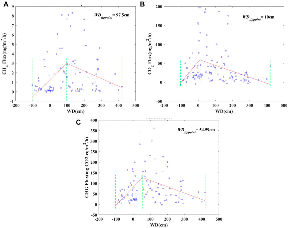
FIGURE 2. Characteristics of carbon fluxes varying with water depth, where CH₄, CO₂ and GHG are shown in Figure 2A, Figure 2B, and Figure 2C, respectively.

Additionally, The GHG varied between −1.70 mg CO₂-eq/m²/h and 360.02 mg CO₂-eq/m²/h, showing a similar pattern in the regression slope with CH₄ and CO₂ fluxes. And the corresponding regression slopes of GHG are 0.848 and −0.301 mg CO₂-eq/m²/h/cm, respectively. Moreover, the turning point of GHG in response to water depth is lower than that of CH₄ and higher than that of CO₂.

3.2 Sensitivity of carbon emission flux varying with water depth

Both CH₄ and CO₂ show the highest sensitivity in 10 cm<WD<97.5 cm, and the sensitivities are 4.89 mg CO₂-eq/m²/h/cm and 4.01 mg CO₂/m²/h/cm, respectively (Figure 3A). The medium and lowest sensitivity of CH₄ and CO₂ occurred when WD<10 cm and WD>97.5 cm, respectively. The sensitivities are 0.52 mg CO₂-eq/m²/h/cm and −0.30 mg CO₂-eq/m²/h/cm for CH₄ emissions varying with water depths of WD<10 cm and WD>97.5 cm, and the sensitivity of CO₂ emissions in the corresponding range of water depths is 0.16 mg CO₂/m²/h/cm and −0.04 mg CO₂/m²/h/cm. Additionally, GHG shows similar results when comparing the magnitude of sensitivity in focused water depth. The sensitivity is 4.51 mg CO₂-eq/m²/h/cm, 0.35 mg CO₂-eq/m²/h/cm and −0.18 mg CO₂-eq/m²/h/cm, where we evaluate the magnitude of the sensitivity on its absolute values.

FIGURE 3

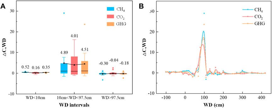
FIGURE 3. Carbon emission sensitivity varying with water depth. Figure 3A shows the average sensitivity of CH₄, CO₂ and GHG in each focused WD interval, and the corresponding emission sensitivity at each water depth is described in Figure 3B.

For the whole water depth of −110 cm–420 cm, CH₄, CO₂ and GHG sensitivity shows a consistent trend with water depth elevation (Figure 3B). Flux sensitivity increased when the water depth was less than the WDT of CH4 (97.5 cm), followed by a declining trend when WD>97.5, and sensitivity remained relatively low at WD>200 cm. The elevation of water depth, from WD<10 cm–10 cm<WD<97.5 cm, shows a positive effect on the CH₄, CO₂ and GHG sensitivities, promoting by 8.48, 23.86 and 11.76 times, respectively. However, CH₄, CO₂ and GHG sensitivities were reduced by nearly 1-fold (0.94–0.99) when the mean water depth was further elevated to WD>97.5 cm.

3.3 Temperature dependence of CH₄ and CO₂ varying with water depth

The results of the correlation analysis of carbon emissions with water depth and temperature showed that CH₄ and CO₂ emission fluxes were correlated with both water depth and temperature (Table 1). Among them, CH₄ was significantly positively correlated with water depth (p<0.01, r=0.267), CO₂ was significantly negatively correlated with water depth (p<0.01, r=-0.419), CH₄ was positively correlated with temperature (p<0.01, 0.427<r<0.565), and the positive correlation between CO₂ and temperature did not reach a significant level (0.071<p<0.253, -0126<r<0.157). In addition, there is no correlation between temperature changes and water depth changes during the sampling period (0.341<p<0.928); that is, in the paired analysis data involved in this study, the change law of carbon emission flux with water depth is not affected by temperature.

TABLE 1

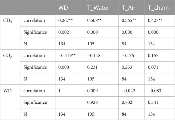
TABLE 1. Correlations of CH₄ and CO₂ with water depth and temperature, where * and ** showed the significant difficance at p < .05 and p < .01.

The CH₄ flux shows a higher temperature dependence than the CO₂ flux, where E_M and E_C for all water depths are 0.69 eV and 0.35 eV (Figure 4), respectively. For the three WD intervals, E_M and E_C showed similar results in 10 cm<WD<97.5 cm and WD>97.5 cm, and E_M was 114.29% and 204.35% higher than E_C. As shown in Figure 5, E_M and E_C in WD<10 cm are 0.42 eV and 0.40 eV, respectively, which are almost the same. The maximum temperature dependence between CH₄ and CO₂ was found at WD>97.5 cm.

FIGURE 4

FIGURE 4. Temperature dependence of CH₄ (Figure 4A) and CO₂ (Figure 4B) emissions.

FIGURE 5

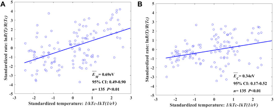
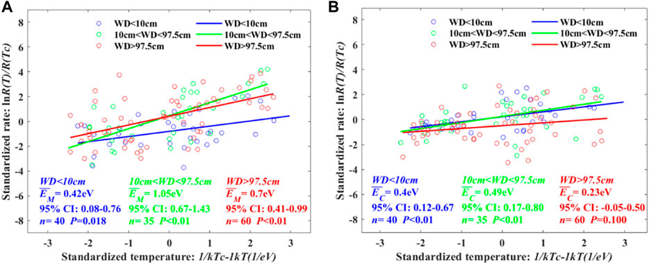
FIGURE 5. Temperature dependence of CH₄ and CO₂ varying with water depth. We evaluated the average temperature dependence at all water depths and separately WD intervals divided by turning points of CH₄ and CO₂ varying with water depth. The temperature independence of CH₄ in WD<10 cm, 10 cm<WD<97.5 cm, and WD>97.5 cm is shown in Figure 5A. The corresponding value of CO₂ is described in Figure 5B.

Both CH₄ and CO₂ temperature dependence show non-monotonic increasing or decreasing trends with water depth elevation or drawdown. For CH₄ temperature dependence in the specific WD intervals, the highest value occurred in 10 cm<WD<97.5 cm, where E_M is 1.05 eV (Table 2). The CH₄ temperature dependence of WD>97.5 cm is higher than that of WD<10 cm, where E_M is 0.70 eV and 0.42 eV, respectively. Additionally, CO₂ temperature dependence indicates the highest E_C in WD 10 cm<WD<97.5 cm, while the EC is lower in WD>97.5 cm than in WD<10 cm.

TABLE 2

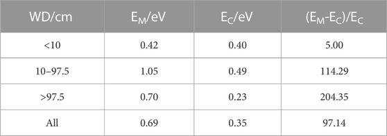
TABLE 2. Temperature dependence of CH₄ and CO₂ in WD intervals.

4 Discussion

4.1 Fluxes and variation sensitivity of carbon emission flux to varying water depth

Turing points at water depths of 97.5 cm and 10 cm for CH₄ and CO₂, respectively, indicate a probable threshold, while the carbon emission flux varies with the fluctuating water level. Redox condition alteration resulting in microbial tolerance and enzymatic activity is one of the main causes (Chimner et al., 2016; Van der Lee et al., 2017). The elevation of water depth increases the ratio of anaerobic microorganisms to aerobic microorganisms, while the overall microbial activity decreases, leading to higher CH₄ emissions and less CO₂ emissions (Jacinthe, 2015; Mader et al., 2017; Li X. et al., 2019; Ye et al., 2019). Additionally, the competition among electron acceptors alters oxidative pathways under oxygen-limited conditions. Recently, Wang et al. (2017) reported that ferrous iron [Fe(II)] has been shown to decrease with a decrease in water levels while also acting as a controlling factor of oxidative phenolic activity. Then, the difference between the relative contributions of CH₄ and CO₂ resulted in a turning point of final GHG emissions at a water depth of 54.6 cm (Holgerson and Raymond, 2016; Zhang et al., 2017; Chen et al., 2021; Huang et al., 2021).

In the range of 10 cm–97.5 cm, CH₄, CO₂ and GHG showed the highest emission flux and sensitivity to varying water depths. As previous studies have shown, emergent vegetation, as part of biological progress, plays a vital role in gas transport from sediment to air and dissolved oxygen changes due to and resistance to hydrodynamic disturbances such as wind and waves in shallow lakes (DelSontro et al., 2018; Tang et al., 2019; Ran et al., 2022). Along the inner range, CH₄ and CO₂ sensitivity increased with the water depth, indicating a positive effect on GHG sensitivity before the water depth reached the tolerance value. As shown in Figures 3A, B positive effect on GHG sensitivity existed in the range of water depths between 10 cm and 97.5 cm, showing that the minimum and maximum tolerance values were out of 10 cm<WD<200 cm. In this study, the sensitivities of CH₄, CO₂ and GHG remained at a low value when the water depth was >200 cm, which also indicated that with a further increase in water depth, the changes in carbon emissions were small.

Therefore, the zone (Z) with a water depth range varying from 10 cm to 97.5 cm may be a more critical zone for reducing carbon emissions through water level control in shallow lakes. Firstly, the highest emission flux reveled that the maximum emission reduction potential can be obtained by controlling the distribution area of Z. Because the potential carbon emission in Z is larger when the area is the same with other zones, and its contribution to the whole lake is greater with increased distribution of Z. Secondly, higher sensitivity to fluctuating water depths indicated that the emission reduction control efficiency is higher with lower cost in management practice, as that increase or decrease amplitude of carbon emission flux in Z, with per unit water depth variation, is larger than other zones. Finally, regulating carbon emissions in Z through adjusting the micro-topography and vegetation distribution is scientific and operable in manage practice (Tang et al., 2019; Liu et al., 2020b), as the crucial role of emergent vegetation and submerged vegetation of Z in carbon emissions by controlling the physical condition and water use (DelSontro et al., 2018; Tang et al., 2019; Ran et al., 2022).

4.2 Temperature dependence of CH₄ and CO₂ varying with water depth

Based on Shelford’s tolerance law (Shelford, 1913; Shelford, 1931; Odum, 1971; Erofeeva, 2021) and metabolic theory (Price et al., 2010), which state that the sensitivity of carbon emissions to varying water depths is temperature-dependent (Chen et al., 2021), this study proved it in specific zones of shallow lakes with water depths varying from 10 cm to 97.5 cm. This study revealed a consistency of carbon emission flux in response to water depth and temperature. CH₄, CO₂ and GHG fluxes show the highest sensitivity to water depth in 10 cm<WD<97.5 cm, and both E_M and E_C are higher than those in other WD intervals. This may be attributed to water depth shifting carbon emissions by adjusting temperature dependence or to additive and interactive effects between water depth and temperature (Birk et al., 2020; Simmons et al., 2021). However, the assumption was not totally verified in WD<10 cm and WD>97.5 cm.

In shallow lakes, for WD<10 cm, dramatic decreasing or elevating water depth shifts anaerobic conditions, and the anaerobic conditions are even broken due to the surface soil being exposed to air (Van der Lee et al., 2017; Jane et al., 2021). Based on the limiting factor principle and metabolic theory, the limitation of water depth restricts the metabolism of organisms related to CH₄ and CO₂, resulting in low temperature dependence and higher sensitivity of CH₄ to water depth (Price et al., 2010; Yvon-Durocher et al., 2014). As shown in this study, the temperature dependence of CH₄ emissions is lowest at WD<10 cm, and E_M is 0.42 eV. However, the difference in CH₄ and CO₂ sensitivity was maximum (108.99%) in this WD interval, and the sensitivity of CH₄ (0.52) to varying water depths was lower than 10 cm<WD<97.5 cm. Additionally, the elevated water depth indicating higher CH₄ and CO₂ sensitivity was additional evidence when WD<10 cm, as shown in Figure 3B.

The pattern of temperature dependence is not totally consistent with the assumption when WD>97.5 cm. Based on this assumption, water depth shifts carbon emissions by adjusting the temperature dependence, E_M and E_C should be higher accordingly when the sensitivity of CH₄, CO₂ and GHG of WD>10 cm is higher than that of WD<97.5 cm. However, compared with WD<10 cm, E_M is indeed increased by 66.67%, while E_C is reduced by -42.50%. Additionally, in WD>97.5 cm, the difference between E_C and E_M reaches a maximum (204.35%), and E_C is lower than the mean value (0.35 eV) at all water depths. Previous studies have shown that CO₂ is an important indicator to characterize the overall activity from microorganisms to ecosystem scales (Price et al., 2010; Yvon-Durocher et al., 2012). A higher water depth may result in an overall metabolic level decline, excluding anaerobic microorganisms correlated with CH₄ (Vicca et al., 2009; Chen et al., 2020).

Above all, there is a specific water depth scope (Figure 6), such as 10 cm<WD<97.5 cm, ensured by the turning point of CH₄ and CO₂, where the temperature dependence of CH₄ and CO₂ is driven by water depth, shifting the GHG emission flux. Additionally, in water-limited conditions and oversaturated conditions with much higher water levels, the impact of temperature on the magnitude and sensitivity of carbon flux is also restricted.

FIGURE 6

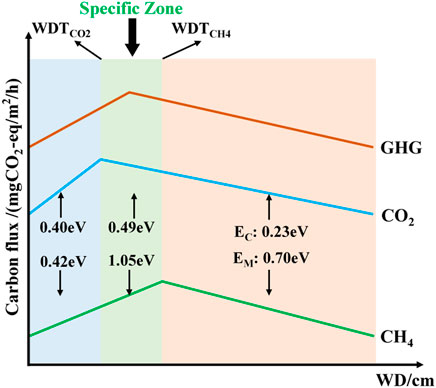
FIGURE 6. Relationship comparison of carbon emissions varying with water depth and carbon emissions responding to temperature.

5 Conclusion

Based on the limiting factor principle of Shelford’s tolerance law and metabolic theory, we explore the threshold while the GHG emission flux varies with water depth in shallow lakes and try to clarify whether the sensitivity of carbon emissions to different water depths is related to temperature. We found that the water depth threshold indicates a maximum CH₄ (97.5 cm) and CO₂ (10 cm), resulting in a water depth threshold of GHG at 54.6 cm. Inter WD intervals, CH₄, CO₂ and GHG in 10 cm<WD<97.5 cm showed the highest emission flux and sensitivity to varying water depths. In the inner WD intervals, the effect of increasing water depth on CH₄, CO₂ and GHG shifted from a positive effect to a negative effect at a WD of 97.5 cm CH₄ and CO₂ sensitivity increase with water depth elevation when WD<97.5 cm, while CH₄ and CO₂ sensitivity show a decreasing trend when WD>97.5 cm. Furthermore, a consistency of carbon emission flux responding to water depth and temperature is only found in specific zones of shallow lakes with 10 cm<WD<97.5 cm, indicating that the temperature dependence of CH₄ and CO₂ are driven by the hydrological regime without water level stress, shifting the GHG emission flux. Linking the result to restoration in shallow lakes, water level control considering seasonal effects on carbon emission reduction is essential. We propose an advice to ensure the goal by governing the time that a turning point occurs and the control costs upon the sensitivity of carbon emissions to unit water depth variation. As we combined samples from multiple dates in this study, it is difficult to clarify short time response and variation of environmental factors, which significantly impacting carbon process. And more sample sites with higher temporal or spatial resolution will improve our understanding of these variations in future research.

Data availability statement

The raw data supporting the conclusions of this article will be made available by the authors. Further inquiries can be directed to the corresponding author.

Author contributions

XY: Methodology, Investigation, Writing–original draft, Writing–review and editing. QL: Conceptualization, Supervision, Funding acquisition, Writing–review. SL: Methodology, Investigation, Writing–original draft. BC: Methodology, Conceptualization. WY: Methodology, Writing–review. TS: Methodology, Conceptualization. XW: Methodology, Investigation. CL: Methodology, Writing–review. YC: Methodology, Conceptualization. ML: Investigation, Visualization. JZ: Methodology, Investigation.

Funding

This study was financially supported by the National Natural Science Foundation of China (No. 42071129, 42271141), and the National Key R&D Program of China (No. 2022YFF1300902).

Conflict of interest

The authors declare that the research was conducted in the absence of any commercial or financial relationships that could be construed as a potential conflict of interest.

Publisher’s note

All claims expressed in this article are solely those of the authors and do not necessarily represent those of their affiliated organizations, or those of the publisher, the editors and the reviewers. Any product that may be evaluated in this article, or claim that may be made by its manufacturer, is not guaranteed or endorsed by the publisher.

Supplementary material

The Supplementary Material for this article can be found online at: https://www.frontiersin.org/articles/10.3389/feart.2022.1086072/full#supplementary-material

Supplementary Figure S1 | Annual mean state of the spatial distribution (Figure S1A) and frequency distribution (Figure S1B) of water depth from 1960 to 2019, and frequency distribution (Figure S1C) of sample sites water depth in field surveys.

References

Birk, S., Chapman, D., Carvalho, L., Spears, B. M., Andersen, H. E., Argillier, C., et al. (2020). Impacts of multiple stressors on freshwater biota across spatial scales and ecosystems. Nat. Ecol. Evol. 4, 1060–1068. doi:10.1038/s41559-020-1216-4

PubMed Abstract | CrossRef Full Text | Google Scholar

CCLCAC (2000). Compilation committee of Local chronicles of Anxin county. Beijing: Xinhua Publishing HouseAnxin county Annals.

Google Scholar

Chen, H., Xu, X., Fang, C., Li, B., and Nie, M. (2021). Differences in the temperature dependence of wetland CO₂ and CH₄ emissions vary with water table depth. Nat. Clim. Chang. 11, 766–771. doi:10.1038/s41558-021-01108-4

CrossRef Full Text | Google Scholar

Chen, H., Zhu, T., Li, B., Fang, C., and Nie, M. (2020). The thermal response of soil microbial methanogenesis decreases in magnitude with changing temperature. Nat. Commun. 11, 5733. doi:10.1038/s41467-020-19549-4

PubMed Abstract | CrossRef Full Text | Google Scholar

Chen, X., Wang, F., Lu, J., Li, H., Zhu, J., and Lv, X. (2017). Simulation of the effect of artificial water transfer on carbon stock of phragmites australis in the baiyangdian wetland, China. Scientifica 2017, 1–11. doi:10.1155/2017/7905710

PubMed Abstract | CrossRef Full Text | Google Scholar

Chimner, R. A., Pypker, T. G., Hribljan, J. A., Moore, P. A., and Waddington, J. M. (2016). Multi-decadal changes in water table levels alter peatland carbon cycling. Ecosystems 20 (5), 1042–1057. doi:10.1007/s10021-016-0092-x

CrossRef Full Text | Google Scholar

Cui, B. S., Han, Z., Li, X., Lan, Y., Bai, J. H., Cai, Y. Z., et al. (2017). Driving mechanism and regulating measures for lake terrestrialization: A case of Lake Baiyangdian. China: Science Press. (In Chinese with English abstract).

Google Scholar

Davidson, N. C. (2014). How much wetland has the world lost? Long-term and recent trends in global wetland area. Mar. Freshw. Res. 65, 934–941. doi:10.1071/MF14173

CrossRef Full Text | Google Scholar

DelSontro, T., del Giorgio, P. A., and Prairie, Y. T. (2018). No longer a paradox: The interaction between physical transport and biological processes explains the spatial distribution of surface water methane within and across lakes. Ecosystems 21, 1073–1087. doi:10.1007/s10021-017-0205-1

CrossRef Full Text | Google Scholar

Erofeeva, E. A. (2021). Plant hormesis and Shelford’s tolerance law curve. J. For. Res. 32, 1789–1802. doi:10.1007/s11676-021-01312-0

CrossRef Full Text | Google Scholar

Evans, C. D., Peacock, M., Baird, A. J., Artz, R. R. E., Burden, A., Callaghan, N., et al. (2021). Overriding water table control on managed peatland greenhouse gas emissions. Nature 593, 548–552. doi:10.1038/s41586-021-03523-1

PubMed Abstract | CrossRef Full Text | Google Scholar

Gao, W., Gao, D., Cai, T., and Liang, H. (2022). Driving factors on greenhouse gas emissions in permafrost region of Daxing'an Mountains, northeast China. J. Geophys. Res. Biogeosciences 127, e2021JG006581. doi:10.1029/2021JG006581

CrossRef Full Text | Google Scholar

Gardner, R. C., Barchiesi, S., Beltrame, C., Finlayson, C. M., Galewski, T., Harrison, I., et al. (2015). State of the world's wetlands and their services to people: A compilation of recent analyses. Brief. Note, 7. doi:10.2139/ssrn.2589447 no.

CrossRef Full Text | Google Scholar

Granberg, G., Mikkela, C., Sundh, I., Svensson, B. H., and Nilsson, M. (1997). Sources of spatial variation in methane emission from mires in northern Sweden: A mechanistic approach in statistical modeling. Glob. Biogeochem. Cycles 11 (2), 135–150. doi:10.1029/96GB03352

CrossRef Full Text | Google Scholar

Hilt, S., Brothers, S., Jeppesen, E., Veraart, A. J., and Kosten, S. (2017). Translating regime shifts in shallow lakes into changes in ecosystem functions and services. BioScience 67 (10), 928–936. doi:10.1093/biosci/bix106

CrossRef Full Text | Google Scholar

Holgerson, M. A., and Raymond, P. A. (2016). Large contribution to inland water CO₂ and CH₄ emissions from very small ponds. Nat. Geosci. 9 (3), 222–226. doi:10.1038/ngeo2654

CrossRef Full Text | Google Scholar

Huang, Y., Ciais, P., Luo, Y., Zhu, D., Wang, Y., Qiu, C., et al. (2021). Tradeoff of CO₂ and CH₄ emissions from global peatlands under water-table drawdown. Nat. Clim. Chang. 11, 618–622. doi:10.1038/s41558-021-01059-w

CrossRef Full Text | Google Scholar

Ise, T., Dunn, A. L., Wofsy, S. C., and Moorcroft, P. R. (2008). High sensitivity of peat decomposition to climate change through water-table feedback. Nat. Geosci. 1 (11), 763–766. doi:10.1038/ngeo331

CrossRef Full Text | Google Scholar

Jaap van der Meer, J. (2006). Metabolic theories in ecology. Trends Ecol. Evol. 21 (3), 136–140. doi:10.1016/j.tree.2005.11.004

PubMed Abstract | CrossRef Full Text | Google Scholar

Jacinthe, P. A. (2015). Carbon dioxide and methane fluxes in variably-flooded riparian forests. Geoderma 241–242, 41–50. doi:10.1016/j.geoderma.2014.10.013

PubMed Abstract | CrossRef Full Text | Google Scholar

Jane, S. F., Hansen, G. J. A., Kraemer, B. M., Leavitt, P. R., Mincer, J. L., North, R. L., et al. (2021). Widespread deoxygenation of temperate lakes. Nature 594, 66–70. doi:10.1038/s41586-021-03550-y

PubMed Abstract | CrossRef Full Text | Google Scholar

Jiang, H. B., Wen, Y., Zou, L. F., Wang, Z., He, C., and Zou, C. (2016). The effects of a wetland restoration project on the Siberian crane (Grus leucogeranus) population and stopover habitat in Momoge National Nature Reserve, China. Ecol. Eng. 96, 170–177. doi:10.1016/j.ecoleng.2016.01.016

CrossRef Full Text | Google Scholar

Kim, D. G., Vargas, R., Bond-Lamberty, B., and Turetsky, M. R. (2012). Effects of soil rewetting and thawing on soil gas fluxes: A review of current literature and suggestions for future research. Biogeosciences 9 (7), 2459–2483. doi:10.5194/bg-9-2459-2012

CrossRef Full Text | Google Scholar

Kong, X., He, Q., Yang, B., He, W., Xu, F., Janssen, A. B. G., et al. (2017). Hydrological regulation drives regime shifts: Evidence from paleolimnology and ecosystem modeling of a large shallow Chinese lake. Glob. Change Biol. 23 (2), 737–754. doi:10.1111/gcb.13416

PubMed Abstract | CrossRef Full Text | Google Scholar

Li, B., Liu, C. Q., Wang, J. X., and Zhang, Y. J. (2009). Carbon storage and fixation function by phragmites australis, a typical vegetation in baiyangdian lake. J. Agro-environment Sci. 28 (12), 2603–2607. (in Chinese with an English abstract).

Google Scholar

Li, X., Yang, W., Sun, T., and Su, L. (2019a). Framework of multidimensional macrobenthos biodiversity to evaluate ecological restoration in wetlands. Environ. Res. Lett. 14 (5), 054003. doi:10.1088/1748-9326/ab142c

CrossRef Full Text | Google Scholar

Li, Y. L., Zhang, Q., Cai, Y. J., Tan, Z., Wu, H., Liu, X., et al. (2019b). Hydrodynamic investigation of surface hydrological connectivity and its effects on the water quality of seasonal lakes: Insights from a complex floodplain setting (Poyang Lake, China). Sci. Total Environ. 660, 245–259. doi:10.1016/j.scitotenv.2019.01.015

PubMed Abstract | CrossRef Full Text | Google Scholar

Liu, F., Liu, J. L., Zhang, T., and Chen, Q. Y. (2010). Land use change and its effects on water quality in Baiyangdian Lake of North China during last 20 years. J. Agro-environment Sci. 10, 1868–1875. (in Chinese with an English abstract).

Google Scholar

Liu, Q., Liu, J. L., Liu, H. F., Liang, L., Cai, Y., Wang, X., et al. (2020b). Vegetation dynamics under water-level fluctuations: Implications for wetland restoration. J. Hydrology 581, 124418. doi:10.1016/j.jhydrol.2019.124418

CrossRef Full Text | Google Scholar

Liu, Q., Ma, X. J., Yan, S. R., Liang, L., Pan, J., and Zhang, J. (2020a). Lag in hydrologic recovery following extreme meteorological drought events: Implications for ecological water requirements. Water 12 (3), 837. doi:10.3390/w12030837

CrossRef Full Text | Google Scholar

Mader, M., Schmidt, C., van Geldern, R., and Barth, J. A. (2017). Dissolved oxygen in water and its stable isotope effects: A review. Chem. Geol. 473, 10–21. doi:10.1016/j.chemgeo.2017.10.003

CrossRef Full Text | Google Scholar

Martínez-Santos, P., de Stefano, L., Llamas, M. R., and Martinez-Alfaro, P. E. (2008). Wetland restoration in the mancha Occidental aquifer, Spain: A critical perspective on water, agricultural, and environmental policies. Restor. Ecol. 16 (3), 511–521. doi:10.1111/j.1526-100X.2008.00410.x

CrossRef Full Text | Google Scholar

Millennium Ecosystem Assessment (2005). Synthesis report. Washington DC: Island.

Google Scholar

Mitsch, W. J., and Gosselink, J. G. (2015). Wetlands. fifth ed. Hoboken, New Jersey: John Wiley & Sons, 747.

Google Scholar

Moor, H., Rydin, H., Hylander, K., Nilsson, M. B., Lindborg, R., and Norberg, J. (2017). Towards a trait-based ecology of wetland vegetation. J. Ecol. 105 (6), 1623–1635. doi:10.1111/1365-2745.12734

CrossRef Full Text | Google Scholar

Odum, E. P. (1971). Fundamentals of ecology. Philadelphia: W.B. Saunders Company.

Google Scholar

Olefeldt, D., Euskirchen, E. S., Harden, J., Kane, E., McGuire, A. D., Waldrop, M. P., et al. (2017). A decade of boreal rich fen greenhouse gas fluxes in response to natural and experimental water table variability. Glob. change Biol. 23 (6), 2428–2440. doi:10.1111/gcb.13612

PubMed Abstract | CrossRef Full Text | Google Scholar

Palmer, M., and Ruhi, A. (2019). Linkages between flow regime, biota, and ecosystem processes: Implications for river restoration. Science 365 (6459), eaaw2087. doi:10.1126/science.aaw2087

PubMed Abstract | CrossRef Full Text | Google Scholar

Poff, N. L., Allan, J. D., Bain, M. B., Karr, J. R., Prestegaard, K. L., Richter, B. D., et al. (1997). The natural flow regime: A paradigm for river conservation and restoration. Bioscience 47, 769–784. doi:10.2307/1313099

CrossRef Full Text | Google Scholar

Price, C. A., Gilooly, J. F., Allen, A. P., Weitz, J. S., and Niklas, K. J. (2010). The metabolic theory of ecology: Prospects and challenges for plant biology. New Phytol. 188 (3), 696–710. doi:10.1111/j.1469-8137.2010.03442.x

PubMed Abstract | CrossRef Full Text | Google Scholar

Ran, L., Wang, X., Li, S., Zhou, Y., Xu, Y., Chan, C. N., et al. (2022). Integrating aquatic and terrestrial carbon fluxes to assess the net landscape carbon balance of a highly erodible semiarid catchment. J. Geophys. Res. Biogeosciences 127, e2021JG006765. doi:10.1029/2021JG006765

CrossRef Full Text | Google Scholar

Shelford, V. E. (1913). Animal communities in a temperate America. Chicago: University of Chicago Press, 386.

Google Scholar

Shelford, V. E. (1931). Some concepts of bioecology. Ecology 12, 455–467. doi:10.2307/1928991

CrossRef Full Text | Google Scholar

Simmons, B. I., Blyth, P. S. A., Blanchard, J. L., Clegg, T., Delmas, E., Garnier, A., et al. (2021). Refocusing multiple stressor research around the targets and scales of ecological impacts. Nat. Ecol. Evol. 5, 1478–1489. doi:10.1038/s41559-021-01547-4

PubMed Abstract | CrossRef Full Text | Google Scholar

Song, C., Xu, X. F., Tian, H., and Wang, Y. (2010). Ecosystem–atmosphere exchange of CH₄ and N₂O and ecosystem respiration in wetlands in the Sanjiang plain, Northeastern China. Glob. Change Biol. 15 (3), 692–705. doi:10.1111/j.1365-2486.2008.01821.x

CrossRef Full Text | Google Scholar

Tang, C., Lei, J., and Nepf, H. M. (2019). Impact of vegetation-generated turbulence on the critical, near bed, wave-velocity for sediment resuspension. Water Resour. Res. 55 (7), 5904–5917. doi:10.1029/2018WR024335

CrossRef Full Text | Google Scholar

Toms, J. D., and Lesperanc, M. L. (2003). Piecewise regression: A tool for identifying ecological thresholds. Ecology 84, 2034–2041. doi:10.1890/02-0472

CrossRef Full Text | Google Scholar

Van der Lee, G. H., Kraak, M. H. S., Verdonschot, R. C. M., Vonk, J. A., and Verdonschot, P. F. M. (2017). Oxygen drives benthic-pelagic decomposition pathways in shallow wetlands. Sci. Rep. 7 (1), 15051. doi:10.1038/s41598-017-15432-3

PubMed Abstract | CrossRef Full Text | Google Scholar

Vicca, S., Janssens, I. A., Flessa, H., Fiedler, S., and Jungkunst, H. F. (2009). Temperature dependence of greenhouse gas emissions from three hydromorphic soils at different groundwater levels. Geobiology 7, 465–476. doi:10.1111/j.1472-4669.2009.00205.x

PubMed Abstract | CrossRef Full Text | Google Scholar

Wang, K. L., Li, H. T., Wu, A. M., Li, M. Z., Zhou, Y., and Li, W. P. (2018). An analysis of the evolution of Baiyangdian wetlands in Hebei Province with artificial recharge. Acta Geol. Sin. 2018 (5), 549–558. doi:10.3975/cagsb.2018.071102

CrossRef Full Text | Google Scholar

Wang, W., Sardans, J., Wang, C., Zeng, C., Tong, C., Bartrons, M., et al. (2018). Shifts in plant and soil C, N and P accumulation and C:N:P stoichiometry associated with flooding intensity in subtropical estuarine wetlands in China. Coast. Shelf Sci. 215, 172–184. doi:10.1016/j.ecss.2018.09.026

CrossRef Full Text | Google Scholar

Wang, Y., Chen, M. J., Yan, L., Yang, G., Ma, J., and Deng, W. (2019). Quantifying threshold water tables for ecological restoration in arid northwestern China. Groundwater 58 (1), 132–142. doi:10.1111/gwat.12934

PubMed Abstract | CrossRef Full Text | Google Scholar

Wang, Y., Wang, H., He, J. S., and Feng, X. (2017). Iron-mediated soil carbon response to water-table decline in an alpine wetland. Nat. Commun. 8, 15972. doi:10.1038/ncomms15972

PubMed Abstract | CrossRef Full Text | Google Scholar

Yang, W., Xu, M. X., Li, R. Q., Zhang, L., and Deng, Q. (2020). Estimating the ecological water levels of shallow lakes: A case study in tangxun lake, China. Sci. Rep. 10, 5637. doi:10.1038/s41598-020-62454-5

PubMed Abstract | CrossRef Full Text | Google Scholar

Yang, Y., McVicar, T. R., Donohue, R. J., Zhang, Y., Roderick, M. L., Chiew, F. H., et al. (2017). Lags in hydrologic recovery following an extreme drought: Assessing the roles of climate and catchment characteristics. Water Resour. Res. 53, 4821–4837. doi:10.1002/2017WR020683

CrossRef Full Text | Google Scholar

Ye, X. C., Meng, Y. K., Xu, L. G., and Xu, C. y. (2019). Net primary productivity dynamics and associated hydrological driving factors in the floodplain wetland of China’s largest freshwater lake. Sci. Total Environ. 659, 302–313. doi:10.1016/j.scitotenv.2018.12.331

PubMed Abstract | CrossRef Full Text | Google Scholar

Yuan, X., Liu, Q., Cui, B. S., Xu, X., Liang, L., Sun, T., et al. (2021). Effect of water-level fluctuations on methane and carbon dioxide dynamics in a shallow lake of Northern China: Implications for wetland restoration. J. Hydrology 597, 126169. doi:10.1016/j.jhydrol.2021.126169

CrossRef Full Text | Google Scholar

Yvon-Durocher, G., Allen, A., Bastviken, D., Conrad, R., Gudasz, C., St-Pierre, A., et al. (2014). Methane fluxes show consistent temperature dependence across microbial to ecosystem scales. Nature 507, 488–491. doi:10.1038/nature13164

PubMed Abstract | CrossRef Full Text | Google Scholar

Yvon-Durocher, G., Caffrey, J., Cescatti, A., Dossena, M., Giorgio, P. d., Gasol, J. M., et al. (2012). Reconciling the temperature dependence of respiration across timescales and ecosystem types. Nature 487, 472–476. doi:10.1038/nature11205

PubMed Abstract | CrossRef Full Text | Google Scholar

Zhang, L., Xia, X., Liu, S., Zhang, S., Li, S., Wang, J., et al. (2020). Significant methane ebullition from alpine permafrost rivers on the East Qinghai–Tibet Plateau. Nat. Geosci. 13, 349–354. doi:10.1038/s41561-020-0571-8

CrossRef Full Text | Google Scholar

Zhang, Z., Zimmermann, N., Stenke, A., Li, X., Hodson, E. L., Zhu, G., et al. (2017). Emerging role of wetland methane emissions in driving 21st century climate change. Proc. Natl. Acad. Sci. 114, 9647–9652. doi:10.1073/pnas.1618765114

PubMed Abstract | CrossRef Full Text | Google Scholar