Joint towed streamer and ocean-bottom-seismometer data multi-parameter full waveform inversion in acoustic-elastic coupled media

Short-offset towed streamer data, and sparse ocean-bottom seismometer (OBS) data are not conducive to applying multi-parameter full waveform inversion (FWI) in production. It is challenging to reconstruct deep velocity in the former, and the latter suffers from severe acquisition footprints. We developed a joint acoustic-elastic coupled full waveform inversion (J-AEFWI) method, in which towed streamer data and ocean-bottom seismometer data were used jointly to build P-wave and S-wave velocity models. A new joint objective function was established using the least-squares theory, and the joint acoustic-elastic coupled full waveform inversion method on the acoustic-elastic coupled equation was derived. The method can inject the residuals of the towed streamer data and the ocean-bottom seismometer data in time backward propagating to update P-wave and S-wave velocity models. The synthetic experimental results show that joint acoustic-elastic coupled full waveform inversion obtains more accurate results than when using these two types of data alone. Compared to using the towed streamer or ocean-bottom seismometer data alone, the joint acoustic-elastic coupled full waveform inversion method leads to better illumination of the deep background velocities and suppression of acquisition footprints. The results of joint acoustic-elastic coupled full waveform inversion were slightly better than those of the cascaded full waveform inversion strategy. To further demonstrate the benefit of the proposed method, we applied it to the field data, and better results are obtained as expected.

1 Introduction

Since it was proposed (Lailly, 1983; Tarantola, 1984), full waveform inversion (FWI) has been successfully applied to practical seismic data to build subsurface geophysical parameters (Crase et al., 1990; Operto et al., 2013; Pan et al., 2018; Pan et al., 2020; Borisov et al., 2020; Peter et al., 2022). In recent decades, the development and application of FWI ranges from acoustic media (Gauthier et al., 1986; Ravaut et al., 2004; Plessix et al., 2010; Xukai and Robert, 2015; Yang et al., 2016) to elastic media (Sears et al., 2008; Vigh et al., 2014; Liu et al., 2021), using towed streamer acquisition (Dessa et al., 2004; Plessix et al., 2010; Shen, 2010) or ocean-bottom node/ocean-bottom seismometer (OBN/OBS) acquisition (Sears et al., 2008; Vigh et al., 2014; Peter et al., 2022).

When OBN/OBSs cannot be deployed on a large scale, a towed streamer is the primary marine seismic wave observation tool. The low cost and low processing effort have appealed to recent researchers and have led to successful cases of acoustic FWI (Dessa et al., 2004; Plessix et al., 2010; Shen, 2010; Agudo et al., 2018); however, several issues need to be addressed. To facilitate macro-model building, FWI relies on a wide-azimuthal acquisition to obtain sufficient transmitted waves (Bunks et al., 1995; Pratt, 1999; Virieux and Operto, 2009; Plessix, 2010). The fixed spreading and cable length limit the towed steamer observation aperture, resulting in insufficient diving waves recorded, especially in deep seawater environments. In this case, FWI tends to fall into cycle skipping without considering other methods to supplement low frequencies (Yao et al., 2019). On the other hand, the modeling equation for acoustic FWI is a simplified approximation of the elastic equation. The converted P-waves generated by the elastic parameters (e.g., S-wave velocity) cannot be simulated using the acoustic equation. When significant converted waves are present in towed streamer data, acoustic FWI tends to incorrectly project converted waves onto P-wave velocity instead of the correct S-wave velocity. Some studies have also focused on this issue, considering that the application of towed streamer data in elastic media in a more advanced approach (Li and Williamson, 2019; Thiel et al., 2019; Sun and Jin, 2020; Yang and Liu, 2020). In addition, the absence of necessary low frequencies and surge noise in streamer data is not conducive to FWI, resulting in the need for other waveform shaping methods.

The multi-parameter elastic FWI for OBN/OBS seismic data is now considered as a more advanced solution to solve some of the complex imaging problems, which usually has the advantages of low frequencies, long offsets, and full azimuthal coverage (Sears et al., 2008; Dellinger et al., 2017; Peter et al., 2022). The benefits of low frequencies need not be elaborated, while the long-offsets and full-azimuthal coverage can receive a sufficient number of diving waves. This weakens the dependence on the starting velocities for obtaining large-scale structures (Plessix et al., 2010). In addition, the abundant S-waves in the OBN/OBS data play a key role in S-wave velocity inversion, which improves the resolution of the multi-parameter inversion results. All of these can overcome the shortcomings of towed streamer acquisition, but limitations of towed streamer cannot be ignored. Its expensive cost and low quantity (hundreds or even thousands of meters apart) constrain its dense deployment in practical production. Insufficient or under-sampled data is not enough for FWI to cover subsurface structures. In general, FWI requires dense, fully sampled data for migration stacking. The under-sampled data, in turn, causes the inversion to fall into a system of underdetermined solutions, causing sharp acquisition footprints and layer discontinuities in the inversion results (Zheglova and Malcolm, 2019; Faucher et al., 2020).

Because OBN/OBS is still expensive to deploy densely, a scheme of a joint towed streamer and OBN/OBS acquisition has been successfully applied (Yang and Zhang, 2019; Yu and Sun, 2022). One of its advantages is that the towed streamer and OBN/OBS simultaneously receive seismic waves from the subsurface (Figure 1). The solid red line indicates the wave path of the towed streamer, and the solid blue line indicates the wave path of the OBS. The OBS is sparsely placed on the seafloor, which can receive P- and S-waves in x, y, and z directions, whereas the densely connected towed streamer hydrophones in seawater can only receive P-waves (containing S-P converted waves). Moreover, their wave paths intuitively showed that OBS acquisition has a larger imaging angle than towed streamer acquisition, and a larger imaging angle is more conducive to FWI macromodel building (Virieux and Operto, 2009). Currently, most FWI applications use only streamer data or OBS data, but few studies use both. We propose a joint acoustic-elastic coupled FWI (J-AEFWI) method that combines towed streamers and OBS data using the acoustic-elastic coupled equation (AECE), which can simultaneously record the pressure component, x, y, and z components in acoustic-elastic coupled media (Yu et al., 2016; Yu and Geng, 2019). The method can inject the residuals of the towed streamer data and the OBS data in time backward propagating to update P-wave and S-wave velocity models. The J-AEFWI approach complements FWI with wide-azimuthal coverage to make obtaining long-wave information easier and make S-wave velocity inversion better than FWI with towed streamer data alone. It complements FWI with dense data simultaneously to suppress the acquisition footprints more than FWI with OBS data alone. Next, the AECE is reviewed, and the J-AEFWI method is illustrated. A set of synthetic and field data inversion experiments were conducted.

FIGURE 1

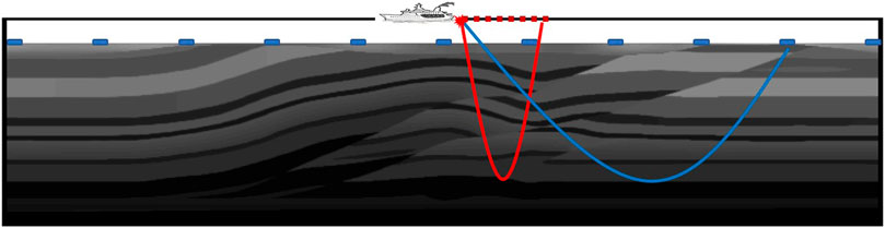
FIGURE 1. Combined towed streamer and OBS acquisition geometry. The red dots on the seawater surface indicate the towed streamer hydrophones, and the blue squares on the sea floor indicate the OBS. The solid red line indicates the wave path of the towed streamer, and the solid blue line indicates the wave path of the OBS.

2 Methodology

In acoustic-elastic coupled media, AECE was used to simulate wave propagation (Yu et al., 2016) as follows:

${\mathbf{L}}_{AE}{\mathbf{U}}_{AE}={\mathbf{F}}_{\mathit{A}\mathit{E}}(1)$

where ${\mathbf{U}}_{AE}={\left(v_x,v_z,P,{\tau }_{xx}^s,{\tau }_{xz}^s\right)}^T$ is the wavefield components and ${\mathbf{F}}_{\mathit{A}\mathit{E}}={\left(\mathrm{0,0},f,\mathrm{0,0}\right)}^T$ is the source vector. $T$ indicates transposition. The operator ${\mathbf{L}}_{AE}$ is the AECE forward operator and satisfies the following:

${\mathbf{L}}_{AE}=\left(\begin{array}{ccccc}\rho \frac{\partial }{\partial t}& 0& \frac{\partial }{\partial x}& -\frac{\partial }{\partial x}& -\frac{\partial }{\partial z}\\ 0& \rho \frac{\partial }{\partial t}& \frac{\partial }{\partial z}& \frac{\partial }{\partial z}& -\frac{\partial }{\partial x}\\ \left(\lambda +\mu \right)\frac{\partial }{\partial x}& \left(\lambda +\mu \right)\frac{\partial }{\partial z}& \frac{\partial }{\partial t}& 0& 0\\ -\mu \frac{\partial }{\partial x}& \mu \frac{\partial }{\partial z}& 0& \frac{\partial }{\partial t}& 0\\ -\mu \frac{\partial }{\partial z}& -\mu \frac{\partial }{\partial x}& 0& 0& \frac{\partial }{\partial t}\end{array}\right)(2)$

where $v_x$ and $v_z$ are the particle velocity components, $P$ is the pressure, ${\tau }_{xx}^s$ and ${\tau }_{xz}^s$ are the deviatoric stress components, $\rho$ is the density, and $\lambda$ and $\mu$ are Lamé parameters. The pressure, x, and z components are integrated into the AECE, allowing pure P-waves to be obtained directly (Yu et al., 2016).

In J-AEFWI, the joint pressure component of the towed streamer and the x and z components of the OBS objective function based on the l₂-norm can be written as

$\underset{m}{\min }J\left(m\right)={\gamma *\mathrm{\phi }\parallel P_{ts}^{sim}-P_{ts}^{obs}\parallel }_2^2+{\alpha \parallel v_{xo}^{sim}-v_{xo}^{obs}\parallel }_2^2+\beta {\parallel v_{zo}^{sim}-v_{zo}^{obs}\parallel }_2^2,(3)$

where $J$ indicates the objective function, $m$ indicates the model parameters, superscripts $sim$ and $obs$ indicate the simulated and observed data, subscripts $ts$, $xo$, and $zo$ indicate the pressure component of the towed streamer, and x and z components of the OBS, respectively.

We used the adjoint-state method to deduce the adjoint equation (included in Appendix A):

${\mathbf{L}}_{AE}^{*}{\stackrel{\sim }{\mathbf{U}}}_{AE}={\stackrel{\sim }{\mathbf{F}}}_{\mathit{A}\mathit{E}}(4)$

where, ${\stackrel{\sim }{\mathbf{U}}}_{AE}={\left({\stackrel{\sim }{v}}_x,{\stackrel{\sim }{v}}_z,\stackrel{\sim }{P},{\stackrel{\sim }{\tau }}_{xx}^s,{\stackrel{\sim }{\tau }}_{xz}^s\right)}^T$ is the adjoint wavefield, ${\mathbf{L}}_{AE}^{*}$ is the adjoint operator, and

${\stackrel{\sim }{\mathbf{F}}}_{\mathit{A}\mathit{E}}={\left(\alpha \left(v_{xo}^{sim}-v_{xo}^{obs}\right),\beta \left(v_{zo}^{sim}-v_{zo}^{obs}\right),\gamma *\mathrm{\phi }\left(P_{ts}^{sim}-P_{ts}^{obs}\right),\mathrm{0,0}\right)}^T(5)$

is the adjoint source function and satisfies

$\left\{\begin{array}{c}\alpha =0,\beta =0,\gamma =1,\mathrm{o}\mathrm{r}\\ \alpha =1,\beta =1,\gamma =0,\mathrm{o}\mathrm{r}\\ \alpha =1,\beta =1,\gamma =1.\end{array}\right.(6)$

Parameters $\alpha$, $\beta$, and $\gamma$ act as switches in the inversions. When $\alpha$ = 0, $\beta$ = 0, and $\gamma$ = 1, it indicated towed streamer data alone. When $\alpha$ = 1, $\beta$ = 1, and $\gamma$ = 0, AEFWI was indicated for OBS data alone. J-AEFWI is indicated when $\alpha$ = 1, $\beta$ = 1, and $\gamma$ = 1. The $\phi$ is a weighting parameter used to control the contribution of different data points in the inversion. The selection strategy for parameter $\phi$ is explained in a subsequent discussion. ${\mathbf{L}}_{AE}^{*}$ was given by:

${\mathbf{L}}_{AE}^{*}=\left(\begin{array}{ccccc}\rho \frac{\partial }{\partial t}& 0& -\frac{\partial }{\partial x}\left(\lambda +\mu \right)& \frac{\partial }{\partial x}\mu & \frac{\partial }{\partial z}\mu \\ 0& \rho \frac{\partial }{\partial t}& -\frac{\partial }{\partial z}\left(\lambda +\mu \right)& -\frac{\partial }{\partial z}\mu & \frac{\partial }{\partial x}\mu \\ -\frac{\partial }{\partial x}& -\frac{\partial }{\partial z}& \frac{\partial }{\partial t}& 0& 0\\ \frac{\partial }{\partial x}& -\frac{\partial }{\partial z}& 0& \frac{\partial }{\partial t}& 0\\ \frac{\partial }{\partial z}& \frac{\partial }{\partial x}& 0& 0& \frac{\partial }{\partial t}\end{array}\right)(7)$

The gradients of the objective function with respect to the parameters $\lambda$ and $\mu$ are derived as follows:

$\left\{\begin{array}{c}\frac{\partial J}{\partial \lambda }={\displaystyle \sum }_{\mathit{s}\mathit{h}\mathit{o}\mathit{t}}\int dt\left(\frac{\partial v_x}{\partial x}+\frac{\partial v_z}{\partial z}\right)\stackrel{\sim }{P}\\ \frac{\partial J}{\partial \mu }={\displaystyle \sum }_{\mathit{s}\mathit{h}\mathit{o}\mathit{t}}\int dt\left(\frac{\partial v_x}{\partial x}+\frac{\partial v_z}{\partial z}\right)\stackrel{\sim }{P}-\left(\frac{\partial v_x}{\partial x}-\frac{\partial v_z}{\partial z}\right){\stackrel{\sim }{\tau }}_{xx}^s-\left(\frac{\partial v_x}{\partial z}+\frac{\partial v_z}{\partial x}\right){\stackrel{\sim }{\tau }}_{xz}^s\end{array}\right.(8)$

Finally, P- and S-wave velocity gradients were obtained using the chain rule. The parameters were updated by:

$m_{k+1}=m_k+{\alpha }_k{g}_k(9)$

where $m$ is the model parameter, $\alpha$ is the updating step length, $g$ is the conjugate update direction of the model parameters, and $k$ is the number of iterations.

3 Synthetic inversion examples

We conducted three FWI experiments for towed streamer data alone, OBS data alone, and combined towed streamer and OBS data. All experiments used Eqs 1, 4, 8, 9 to invert P- and S-wave velocities, and the difference is the selection of the weighting parameters in Eq. 6. The size of the true and starting models was 10 km × 3.5 km shown in Figure 2. The experimental acquisitions followed the towed streamer and the OBS acquisition. A total of 200 streamer hydrophones were spaced 20 m apart at the seawater surface, and 11 OBS were spaced 1,000 m apart on the seafloor. Figure 3 shows the common shot gathers for both acquisitions. The towed streamer data had a clear acquisition density advantage, but only a few diving waves were recorded. In contrast, OBS data are sparse, but its long-offset data are abundant. The experiments are concerned with P-wave velocity and S-wave velocity building, and the weak parameter density is the true value that is not updated in the inversions. All three experiments were iterated 200 times to maintain consistency in the computation effort.

FIGURE 2

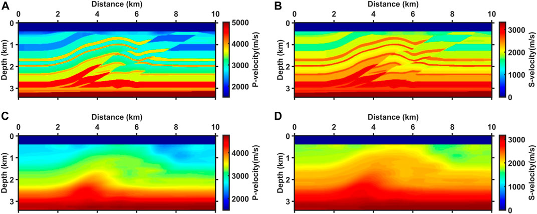
FIGURE 2. The true P-wave velocity (A) and S-wave velocity (B) models and their starting models (C,D).

FIGURE 3

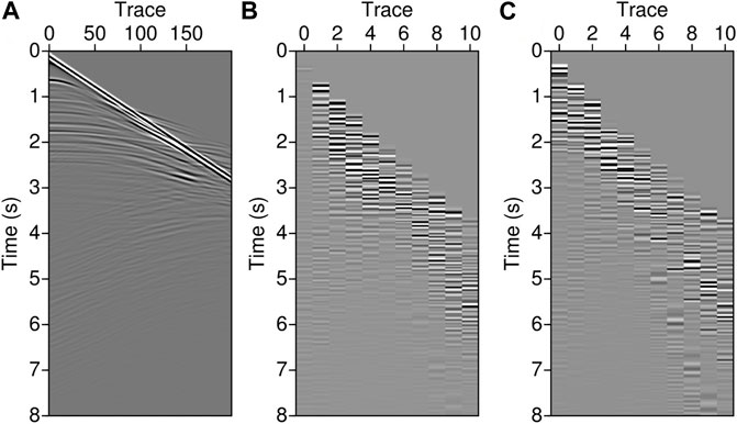
FIGURE 3. Shot gathers of the towed streamer (A), OBS x (B), and z (C) components.

The characteristics of these three experiments can be observed in the updated directions for the first iteration of the inversion, as shown in Figure 4. Figures 4A, B show the P-wave velocity and S-wave velocity updating directions of the AEFWI for towed streamer data. The updating direction of the P-wave velocity has good continuity of layers (especially in shallow parts), which is attributed to the dense acquisition of the towed streamer. The weakness of (A) is that the updating direction is dominated by the high-wavenumber information mainly concentrated on the layers rather than the most desired low-wavenumber information. This is because of the slight imaging angle, which is attributed to the narrow aperture of the towed streamer acquisition. Although FWI can slowly recover models after multiple iterations, such small-angle data are unfavorable for inversion. Moreover, relying only on small-angle reflected waves, the illumination of the shallow part of the updating direction is excellent, whereas the illumination of the deep part is insufficient (Peter et al., 2022). In addition, without S-waves, the direction of the S-wave velocity relying only on the converted P-waves is insufficient and shows dispersion in depth.

FIGURE 4

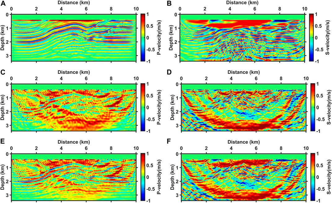
FIGURE 4. The P-wave velocity (A,C,E) and S-wave velocity (B,D,F) updating directions for the first iteration of three inversion experiments. (A,B) are updating directions of towed streamer data alone, (C,D) are updating directions of OBS data alone, and (E,F) are updating directions of joint towed streamer and OBS data.

Figure 4C, D show P-wave and S-wave velocity updating directions of sparse OBS data AEFWI. As expected, the updating directions of the OBS data are very poor for layer continuity compared with the updating directions of the towed streamer data. The sparse data indicate that imaging stacking is insufficient, and many acquisition footprints (show arcs) appear in the direction profiles. Encouragingly, long-offset data play a significant role in determining the background velocity. The updated directions of the OBS data have more low-wavenumber information, which is crucial for recovering large-scale structures. The deep illumination of the model is much better because of wide-azimuthal acquisition (Shen et al., 2018). Virieux and Operto (2009) found that the frequency and imaging angle influence the wavenumber of the imaging. The lower the frequencies and the larger the imaging angles, the lower the wavenumber of the imaging results. If the starting model is not good enough, the low frequency and long observation aperture become keys to the success of FWI (Shipp and Singh, 2002; Ravaut et al., 2004; Operto et al., 2006; Plessix et al., 2010). In addition, positively influenced by the abundant S-waves, the updating direction of the S-wave velocity is better illuminated in the deep part (Figure 4D), making the S-wave velocity inversion more likely to succeed (Ren and Liu, 2016; Wang and Cheng, 2017).

Figures 4E, F show the P-wave and S-wave velocity updating directions of the J-AEFWI. The updating directions of J-AEFWI are shaped as a combination of the towed streamer and OBS updating directions. On the one hand, the strong acquisition footprints are faded, and the continuity of the layers was enhanced owing to the addition of the towed streamer data. On the other hand, the low-wavenumber information from the wide-azimuthal OBS data remained, and the superior illumination of the deep parts was preserved. As observed, the updated directions of J-AEFWI carry more information for P-wave and S-wave velocity buildings.

Figure 5 shows the wavenumber spectrum of the updating directions of the FWI for towed streamer data, OBS data and J-AEFWI. The low wavenumbers in the updating directions of the OBS data are dominant, whereas updating the directions of the towed streamer data contain higher wavenumbers. The updating directions of J-AEFWI contain both low and high wavenumbers.

FIGURE 5

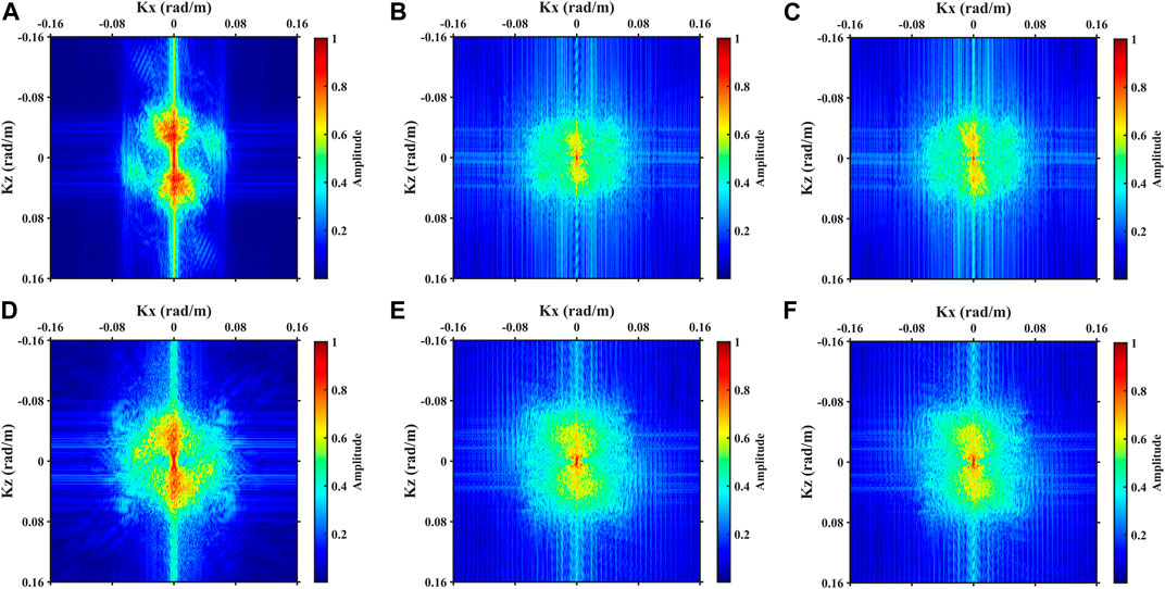
FIGURE 5. The spectrums of updating directions. (A–C) are the P-wave velocity updating direction of TS-FWI, OBS-FWI and J-AEFWI, respectively. (D–F) are the S-wave velocity updating direction of TS-FWI, OBS-FWI and J-AEFWI, respectively.

The characteristics of the updating directions are projected in the inversion results. Figure 6 shows the results of the three inversion experiments. Figures 6A, B are P-wave and S-wave velocity results for the towed streamer data. Benefiting from dense acquisition, FWI accurately depicts the structural layers, which are almost consistent with the true velocities. However, below 2 km depth, the different background velocities are not adequately inverted and blended, which affects the identification of deeper structures (low-velocity structures indicated by the dashed boxes). In the results of the OBS data (Figures 6C, D), large-scale background velocities are adequately inverted, especially at the depth indicated by the dashed boxes, where the low-velocity structures are well illuminated and can be identified clearly. The shortcoming is that insufficient data leads to inadequate stacking, resulting in poor continuity and shallow acquisition footprints. Figures 6E, F show better inversion results for J-AEFWI. In the shallow part, the results depict the layers at high resolution, and the acquisition footprints are suppressed; in the deep part, sufficient illumination and accurate macroscopic velocities remain.

FIGURE 6

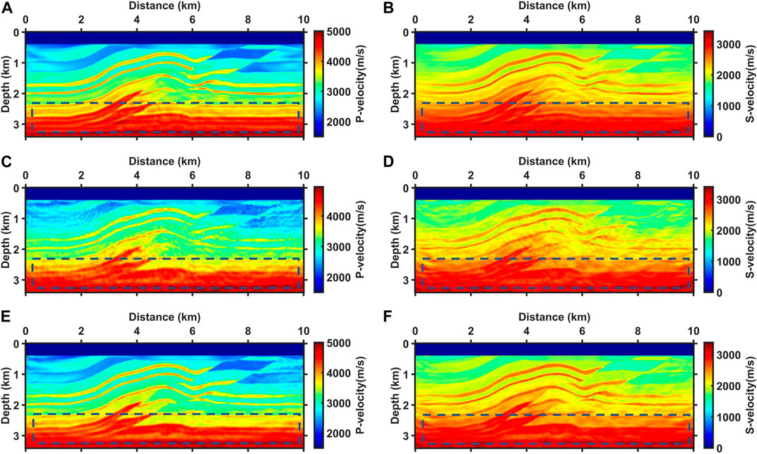
FIGURE 6. The P-wave velocity (A,C,E) and S-wave velocity (B,D,F) inversion results. (A,B) are results for towed streamer data alone, (C,D) are results for OBS data alone, (E,F) are results for joint towed streamer and OBS data.

Figure 7 shows vertical velocity profiles at three different locations. Above 2 km depth, the results for towed streamer data (red lines) closely match true velocities (black lines), while the results deviate from true velocities below it. On the contrary, the results for OBS data (green lines) are slightly worse at shallow depth and slightly better at a deeper depth. The inversion results of J-AEFWI accurately fit the true velocities in both the deep and shallow parts. Overall, the results of J-AEFWI are better than those of AEFWI for towed streamer data alone or AEFWI for OBS data alone.

FIGURE 7

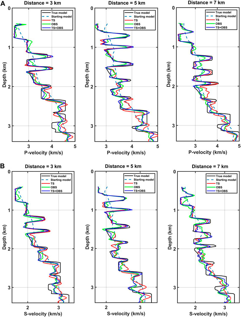
FIGURE 7. Vertical P-wave velocity (A) and S-wave velocity (B) profiles at three different locations. The solid black lines indicate the true velocities, the dashed lines indicate the starting velocities, the red lines indicate the results for towed streamer data, the green lines indicate the results for OBS data, and the blue lines indicate the J-AEFWI results.

To further illustrate the accuracy of the inversion results, the data residuals are quantitatively shown. Figure 8 shows the final data residuals of FWI for towed streamer data, OBS data, and J-AEFWI. Where the red arrows indicate, the amplitudes of residuals are smaller for J-AEFWI. Compared to the residuals of the initial model, the data residuals of the final inversion results are shown in Table 1. Naturally, the FWI for towed streamer data uses only towed streamer data and not the OBS data, which has the smallest residuals for the towed streamer data and the larger residuals for the OBS data. The FWI for OBS data uses only OBS data and not the towed streamer data, which has the smallest residuals for the OBS data and the larger residuals for the towed streamer data. The J-AEFWI uses both towed streamer and OBS data, and have the smallest residuals.

FIGURE 8

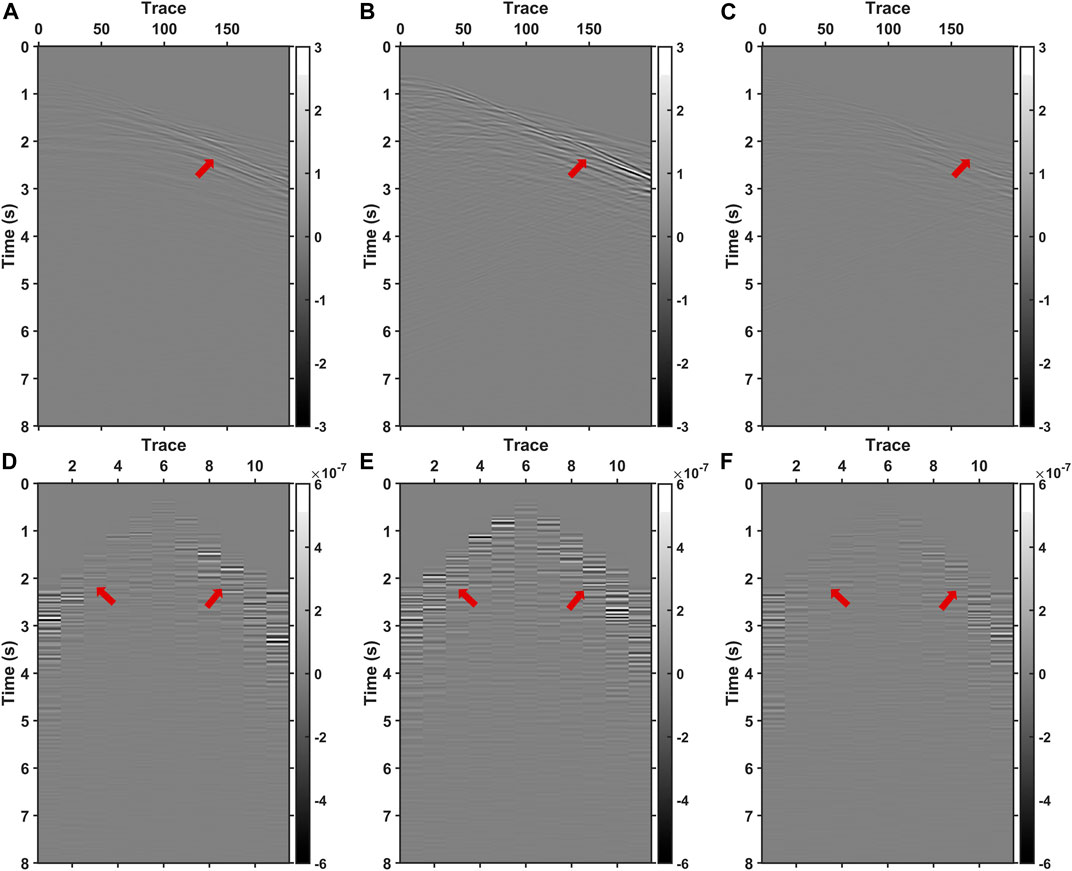
FIGURE 8. Pressure residuals of FWI results for (A) towed streamer data, (B) OBS data and (C) J-AEFWI. The z-components residuals of FWI results for (D) towed streamer data, (E) OBS data and (F) J-AEFWI.

TABLE 1

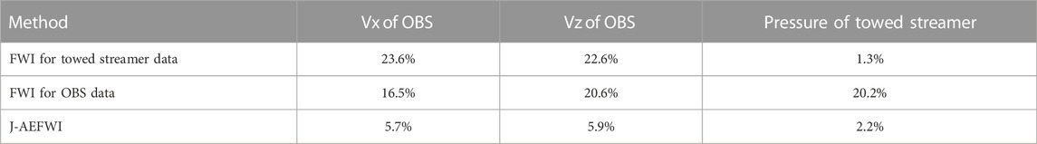
TABLE 1. The data residuals of the final inversion results.

4 Field data examples

We tested the J-AEFWI approach on South China Sea field data. A total of 875 shots were distributed evenly over a straight line of approximately 20 km. Considering the calculation cost, we selected only a part of the data to implement in the experiments. The collection ship carried 360 towed streamer hydrophones, and only five OBSs were arranged on the seafloor with 400 m spacing. Figure 9 shows the x, z-component of an OBS, and the towed streamer data. We know from early works that free gas layers exist in the target area (indicated by the yellow line in Figure 10A). During pre-processing, we applied a transformation from 3D to 2D geometric spreading (Crase et al., 1990), and a band-pass filter was applied to the data. A time window is applied to mute the reflected waves after multiple arrivals.

FIGURE 9

FIGURE 9. The x, z-component data of OBS and towed streamer data.

FIGURE 10

FIGURE 10. The starting P-wave (A) and S-wave (B) velocities; P-wave (C) and S-wave (D) velocities of AEFWI for OBS data; and P-wave (E) and S-wave (F) velocities of J-AEFWI. The dotted line behind the ship indicates the towed streamer, the red balls represent OBS, and the target area is in the red box. The yellow line indicates the free gas layer. The part of images of starting P-wave velocity (G), starting S-wave velocity (H), P-wave velocity of AEFWI for OBS data (I), S-wave velocity of AEFWI for OBS data (J), P-wave velocity of J-AEFWI (K) and S-wave velocity of J-AEFWI (L), respectively. The areas indicated by arrows, rectangles and circles show improvements for J-AEFWI.

In approximately 1 km deep water, the towed streamer hardly received the diving waves, so it is unwise to implement FWI for multi-parameter building using towed streamer data alone. In this section, we describe the implementation of an AEFWI experiment for OBS data and a J-AEFWI experiment. The starting P-wave and S-wave models are presented in Figures 10A, B. Before the FWI, we improved the starting models using tomography techniques.

Figures 10C, D shows AEFWI results for OBS data alone. Compared with the starting models, the inversion results change on macroscopic velocities and appear to have some high wavenumber information which is beneficial to identify the layers. In particular, a well-defined low-velocity layer appears in the shallow part, which is consistent with prior information provided by the early works that free gas layers exist in the target area. Unfortunately, sparse data led to poor continuity and irregular perturbations in these layers. J-AEFWI improved these anomalies caused by insufficient data. As shown in Figures 10E, F, the irregular disturbances of the layers are suppressed, and layers are more continuous.

Conventionally, the reverse time migration (RTM) imaging technique is used to verify the accuracy of inversion results. Figures 10G–L shows the P-wave velocity (G) and S-wave velocity (H) images of the starting models, P-wave velocity (I) and S-wave velocity (J) images of AEFWI for OBS data, and P-wave velocity (K) and S-wave velocity (L) images of J-AEFWI. In the target area, both inversion experiments improved the RTM images (indicated by rectangular areas). More accurate velocities allowed the images to migrate to the correct position, as evidenced by the more continuous and clear images. In particular, the images of S-wave velocities, which were blurred for the starting models, improved significantly with the inversion results. In addition, the images of the J-AEFWI results are more converged and clearer than those of the OBS data (indicated by the circles and arrows).

Figure 11 presents a comparison between field data and synthetic data for the initial models, OBS data AEFWI results, and J-AEFWI results. The center of the red lines represents the field data, with the synthetic data on either side. The waveforms after multiples have been suppressed. In Figure 11A, the initial model’s synthetic data lacks some reflection events and exhibits poor continuity (as indicated by the red arrow). In contrast, Figure 11B demonstrates that the OBS data inversion results exhibit improved continuity in the reflection events. Finally, Figure 11C shows that the synthetic data generated by the J-AEFWI method most closely aligns with the field data, as indicated by the red circles.

FIGURE 11

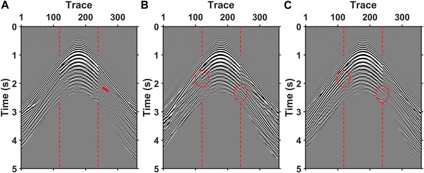
FIGURE 11. Synthetic data generated using initial models (A), AEFWI results for OBS data (B) and J-AEFWI results, compared to the observed data. The middle of each image shows the field data and the sides show the synthetic data, which are separated by red lines. The waveforms after multiples are muted.

To verify the reliability of the inversion results, we show the P-wave and S-wave velocity images with a velocity model overlay, as shown in Figures 12A–D, where the emerging velocity layers largely coincide with the image positions. We also show the angle-domain common-image gathers (ADCIGs) to illustrate the accuracy of the inversion results. Figures 12E–H shows ADCIGs at locations in the target region. Figures 12E–F show the ADCIGs of P-wave velocity and S-wave velocity for the AEFWI of OBS data, and Figures 12G–H show the ADCIGs of P-wave velocity and S-wave velocity for the AEFWI of joint data. The ADCIGs of the two FWIs are generally similar, and a comparison shows that the ADCIGs of the J-AEFWI results are flatter and clearer at some locations than those of the OBS data (indicated by arrows and rectangles).

FIGURE 12

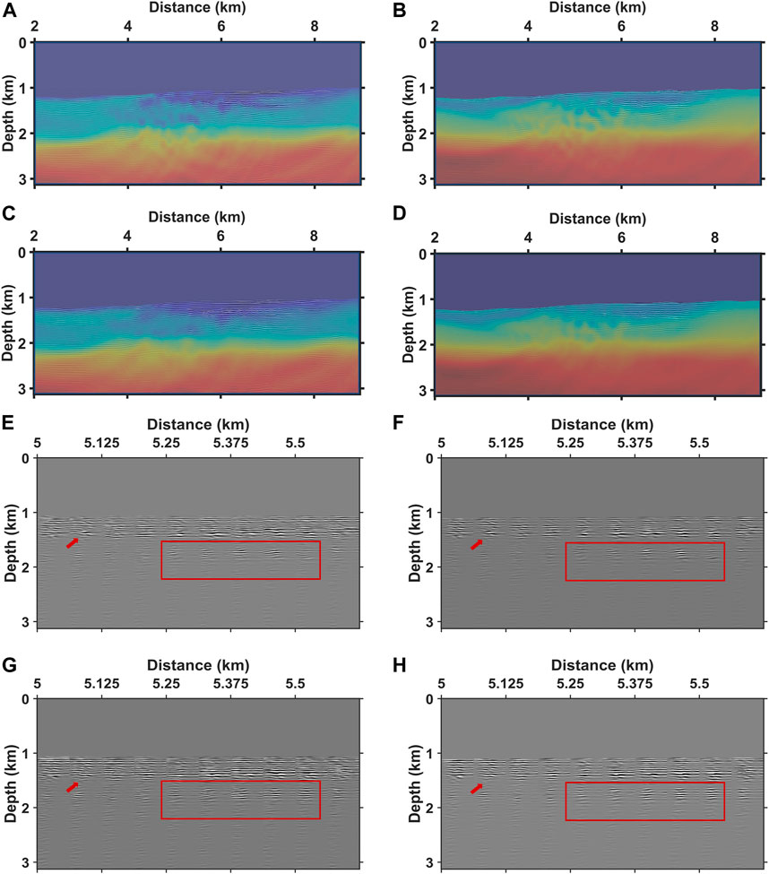
FIGURE 12. The images with corresponding velocity models overlay. P-wave velocity of AEFWI for OBS data (A), S-wave velocity of AEFWI for OBS data (B), P-wave velocity of J-AEFWI (C) and S-wave velocity of J-AEFWI (D). The ADCIGs of (E) P-wave velocity of AEFWI for OBS data, (F) S-wave velocity of AEFWI for OBS data, (G) P-wave velocity of J-AEFWI, and (H) S-wave velocity of J-AEFWI. The areas indicated by arrows and rectangles show improvements for J-AEFWI.

5 Discussion

The weighting parameter $\phi$ played a key role in the success of the J-AEFWI approach. For simplicity, the value of $\phi$ was set to balance the proportions of the two data in the objective function. In addition, before calculating the updating directions of J-AEFWI, $\phi$ can be adjusted such that the energy of the gradients of the two types of data is approximately half. In practice, the value of $\phi$ can be adjusted according to the quality of the different data. If the spacing of OBS in the field data is large, it is appropriate to increase the weighting of towed streamer data and decrease the weighting of OBS data in this case. The weighting of the OBS data can be increased as the OBS interval decreases, or the weighting of the towed streamer data can be adjusted downward if the noise pollution is serious.

Next, we present a cascaded AEFWI approach that does not require determining the value of the weighting parameters. We first inverted 100 times using the OBS data, and the inversion results were then inverted 100 times using the towed streamer data, with the same inversion parameters as above for AEFWI. As shown in Figure 13, the cascaded AEFWI accurately reconstructs the velocity models. In the vertical velocity profiles (Figure 14), the inversion accuracy of the cascaded FWI was slightly worse than that of J-AEFWI. This is because cascaded FWI utilizes both data in segments, whereas J-AEFWI utilizes both data in the entire inversion process.

FIGURE 13

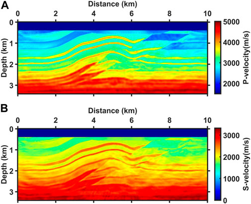
FIGURE 13. P-wave (A) and S-wave (B) velocity of cascaded AEFWI.

FIGURE 14

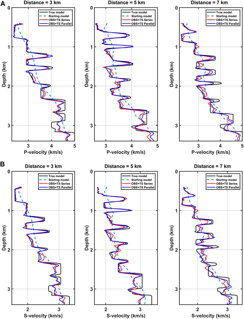
FIGURE 14. Vertical P-wave velocity (A) and S-wave velocity (B) profiles at three different locations. The solid black lines indicate the true velocities, the dashed lines indicate the starting velocities, the red lines indicate the cascaded AEFWI results, and the blue lines indicate the J-AEFWI results.

Figure 15 shows P-wave and S-wave velocity normalized misfits between inversion and true models. First, the decline of J-AEFWI in P-wave velocity misfit is leading in the whole process, and cascaded AEFWI takes inversion results of OBS data as the starting point, which inevitably lags behind J-AEFWI. This pattern is the same in S-wave velocity misfit, but inversion for OBS data is ahead of inversion for towed streamer data. This is because S-waves in OBS data play a significant role in S-wave velocity building.

FIGURE 15

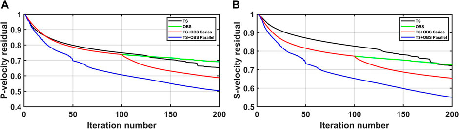
FIGURE 15. P-wave (A) and S-wave (B) velocity normalized misfits between inversion and true models. Black lines indicate AEFWI for towed streamer data; green lines indicate AEFWI for OBS data; red lines indicate cascaded AEFWI; blue lines indicate J-AEFWI.

6 Conclusion

We developed a J-AEFWI method, in which towed streamer and OBS data were used to build P-wave and S-wave velocity models based on the same acoustic-elastic coupled equations. This method combines the advantages of both types of data. On the one hand, towed streamer data with dense acquisition can accurately depict model layers and suppress acquisition footprints. On the other hand, the long-offset OBS data with rich diving waves benefit deep illumination and large-scale background velocity building. The synthetic experimental results show that J-AEFWI obtains more accurate results than when using these two types of data alone. The results of J-AEFWI were slightly better than those of the cascaded FWI strategy. This method was applied to the field data, and better results were obtained.

Data availability statement

The original contributions presented in the study are included in the article/supplementary material, further inquiries can be directed to the corresponding author.

Author contributions

TY: investigation, methodology and writing manuscript. YL and JY: checking and modifying manuscript.

Funding

We are grateful for financial support from National Natural Science Foundation of China (grant nos 41930105; 41774122; 41630964; 41874127; 42004096), the National Key R&D Program of China (grant nos 2018YFC0310100 and 2019YFC0312004), the Fundamental Research Funds for the Central Universities of China, and the Strategic Priority Research Program of the Chinese Academy of Sciences (grant no. XDA14010203).

Conflict of interest

The authors declare that the research was conducted in the absence of any commercial or financial relationships that could be construed as a potential conflict of interest.

Publisher’s note

All claims expressed in this article are solely those of the authors and do not necessarily represent those of their affiliated organizations, or those of the publisher, the editors and the reviewers. Any product that may be evaluated in this article, or claim that may be made by its manufacturer, is not guaranteed or endorsed by the publisher.

References

Agudo, O. C., da Silva, N. V., Warner, M., and Morgan, J. (2018). Acoustic full-waveform inversion in an elastic world. Geophysics 83 (3), R257–R271. doi:10.1190/geo2017-0063.1

CrossRef Full Text | Google Scholar

Borisov, D., Gao, F., Williamson, P., and Tromp, J. (2020). Application of 2D full-waveform inversion on exploration land data. Geophysics 85 (2), R75–R86. doi:10.1190/geo2019-0082.1

CrossRef Full Text | Google Scholar

Bunks, C., Saleck, F. M., Zaleski, S., and Chavent, G. (1995). Multiscale seismic waveform inversion. Geophysics 60, 1457–1473. doi:10.1190/1.1443880

CrossRef Full Text | Google Scholar

Crase, E., Pica, A., Noble, M., McDonald, J., and Tarantola, A. (1990). Robust elastic nonlinear waveform inversion: Application to real data. Geophysics 55, 527–538. doi:10.1190/1.1442864

CrossRef Full Text | Google Scholar

Dessa, J. -X., Operto, S., Kodaira, S., Nakanishi, A., Pascal, J., Virieux, J., et al. (2004). Multiscale seismic imaging of the eastern Nankai trough by full waveform inversion. Geophys. Res. Lett. 31, L18606. doi:10.1029/2004GL020453

CrossRef Full Text | Google Scholar

Dellinger, J., Brenders, A., Sandschaper, J. R., Regone, C., Etgen, J., Ahmed, S., et al. (2017). The Garden Banks model experience. The Leading Edge 36, 151–158. doi:10.1190/tle36020151.1

CrossRef Full Text | Google Scholar

Faucher, F., Alessandrini, G., Barucq, H., de Hoop, M. V., Gaburro, R., and Sincich, E. (2020). Full reciprocity-gap waveform inversion enabling sparse-source acquisition. Geophysics 85 (6), R461–R476. doi:10.1190/GEO2019-0527.1

CrossRef Full Text | Google Scholar

Gauthier, O., Virieux, J., and Tarantola, A. (1986). Two-dimensional nonlinear inversion of seismic waveforms: numerical results. Geophysics 51 (7), 1387.

CrossRef Full Text | Google Scholar

Lailly, P. (1983). The Seismic Inverse Problem as a Sequence of Before Stack Migrations: Conference on Inverse Scattering: Theory and Application. Expanded Abstracts: SEG. New Delhi, India: SIAM, 206–220.

Google Scholar

Lanzarone, P., Shen, X., Brenders, A., Xia, G., Dellinger, J., Ritter, G., et al. (2022). Innovative application of full-waveform inversion applied to extended wide-azimuth marine streamer seismic data in a complex salt environment. Geophysics 87 (3), B193–B205. doi:10.1190/geo2021-0374.1

CrossRef Full Text | Google Scholar

Li, D., Gao, F., and Williamson, P. (2019). A Deep Learning Approach for Acoustic FWI With Elastic Data: 89th Annual International Meeting. Expanded Abstracts: SEG, New Delhi, India. 2303–2307.

Google Scholar

Liu, Y., Huang, X., Yang, J., Liu, X., Li, B., Dong, L., et al. (2021). Multiparameter model building for the Qiuyue structure using 4C ocean-bottom seismometer data. Geophysics 86, B291–B301. doi:10.1190/geo2020-0537.1

CrossRef Full Text | Google Scholar

Operto, S., Gholami, Y., Prieux, V., Ribodetti, A., Brossier, R., Metivier, L., et al. (2013). A guided tour of multiparameter full-waveform inversion with multicomponent data: From theory to practice. Lead. EDGE 32, 1040–1054. doi:10.1190/tle32091040.1

CrossRef Full Text | Google Scholar

Operto, S., Virieux, J., Dessa, J. -X., and Pascal, G. (2006). Crustal seismic imaging from multifold ocean bottom seismometer data by frequency domain full waveform tomography: Application to the eastern Nankai trough. J. Geophys. Res. SOLID EARTH 111, B09306. doi:10.1029/2005JB003835

CrossRef Full Text | Google Scholar

Pan, W., Geng, Y., and Innanen, K. A. (2018). Interparameter trade-off quantification and reduction in isotropic-elastic full-waveform inversion: Synthetic experiments and hussar land data set application. Geophys. J. Int. 212, 1305–1333. doi:10.1093/gji/ggy037

CrossRef Full Text | Google Scholar

Pan, W., Innanen, K. A., and Wang, Y. (2020). Parameterization analysis and field validation of VTI-elastic full-waveform inversion in a walk-away vertical seismic profile configuration. Geophysics 85 (3), B87–B107. doi:10.1190/geo2019-0089.1

CrossRef Full Text | Google Scholar

Peter, L., Xukai, S., Andrew, B., Ganyuan, X., Joe, D., Gabriel, R., et al. (2022). Innovative application of full-waveform inversion applied to extended wide-azimuth marine streamer seismic data in a complex salt environment. Geophysics 87, B193–B205. doi:10.1190/geo2021-0374.1

CrossRef Full Text | Google Scholar

Plessix, R. E., Baeten, G., de Maag, J. W., Klaassen, M., Rujie, Z., and Zhifei, T. (2010). Application of Acoustic Full Waveform Inversion to a Low-Frequency Large-Offset Land Data Set: 2010 Annual Meeting. Expanded Abstracts: SEG, New Delhi, India, 930–934.

Google Scholar

Pratt, R. G. (1999). Seismic waveform inversion in the frequency domain, Part 1: Theory and verification in a physical scale model. Geophysics 64, 888–901. doi:10.1190/1.1444597

CrossRef Full Text | Google Scholar

Ravaut, C., Operto, S., Improta, L., Virieux, J., Herrero, A., and Dell'Aversana, P. (2004). Multiscale imaging of complex structures from multifold wide-aperture seismic data by frequency-domain full-waveform tomography: Application to a thrust belt. Geophys. J. Int. 159, 1032–1056. doi:10.1111/j.1365-246X.2004.02442.x

CrossRef Full Text | Google Scholar

Ren, Z., and Liu, Y. (2016). A hierarchical elastic full-waveform inversion scheme based on wavefield separation and the multistep-length approach. Geophysics 81 (3), R99–R123. doi:10.1190/geo2015-0431.1

CrossRef Full Text | Google Scholar

Sears, T. J., Singh, S. C., and Barton, P. J. (2008). Elastic full waveform inversion of multi-component OBC seismic data. Geophys. Prospect. 56, 843–862. doi:10.1111/j.1365-2478.2008.00692.x

CrossRef Full Text | Google Scholar

Shen, X., Ahmed, I., Brenders, A., Dellinger, J., Etgen, J., and Michell, S. (2018). Full-waveform inversion: The next leap forward in subsalt imaging. Lead. EDGE 37, 67b1–67b6. doi:10.1190/tle37010067b1.1

CrossRef Full Text | Google Scholar

Shen, X., and Clapp, R. G. (2015). Random boundary condition for memory-efficient waveform inversion gradient computation. Geophysics 80, R351–R359. –R359. doi:10.1190/geo2014-0542.1

CrossRef Full Text | Google Scholar

Shen, X. (2010). Near-Surface Velocity Estimation by Weighted Early-Arrival Waveform Inversion: 2010 Annual Meeting. Expanded Abstracts: SEG, New Delhi, India.

Google Scholar

Shipp, R. M., and Singh, S. C. (2002). Two-dimensional full wavefield inversion of wide-aperture marine seismic streamer data. Geophys. J. Int. 151, 325–344. doi:10.1046/j.1365-246X.2002.01645.x

CrossRef Full Text | Google Scholar

Sun, M., and Jin, S. (2020). Multiparameter elastic full waveform inversion of ocean bottom seismic four-component data based on a modified acoustic-elastic coupled equation. Remote Sens. 12, 2816. doi:10.3390/rs12172816

CrossRef Full Text | Google Scholar

Tarantola, A. (1984). Inversion of seismic reflection data in the acoustic approximation. Geophysics 49, 1259–1266. doi:10.1190/1.1441754

CrossRef Full Text | Google Scholar

Thiel, N., Hertweck, T., and Bohlen, T. (2019). Comparison of acoustic and elastic full waveform inversion of 2D towed-streamer data in the presence of salt. Geophys. Prospect. 67, 1365-2478.12728–361. doi:10.1111/1365-2478.12728

CrossRef Full Text | Google Scholar

Vigh, D., Jiao, K., Watts, D., and Sun, D. (2014). Elastic full-waveform inversion application using multicomponent measurements of seismic data collection. Geophysics 79, R63–R77. doi:10.1190/geo2013-0055.1

CrossRef Full Text | Google Scholar

Virieux, J., and Operto, S. (2009). An overview of full-waveform inversion in exploration geophysics. Geophysics 74, WCC1–WCC26. doi:10.1190/1.3238367

CrossRef Full Text | Google Scholar

Wang, T. F., and Cheng, J. B. (2017). Elastic full waveform inversion based on mode decomposition: The approach and mechanism. Geophys. J. Int. 209, 606–622. doi:10.1093/gji/ggx038

CrossRef Full Text | Google Scholar

Yang, H., and Zhang, J. (2019). Full waveform inversion of combined towed streamer and limited OBS seismic data: A theoretical study. Mar. Geophys. Res. 40, 237–244. doi:10.1007/s11001-018-9363-6

CrossRef Full Text | Google Scholar

Yang, J., Liu, Y., and Dong, L. (2016). Simultaneous estimation of velocity and density in acoustic multiparameter full-waveform inversion using an improved scattering-integral approach. GEOPHYSICS 81, R399–R415. doi:10.1190/geo2015-0707.1

CrossRef Full Text | Google Scholar

Yang, T., and Liu, Y. (2020). Full waveform inversion based on the acoustic-elastic coupled equation. 2020 Annu. Conf. Exhib. OnlineEAGE 2020, 1–5. doi:10.3997/2214-4609.202010563

CrossRef Full Text | Google Scholar

Yao, G., da Silva, N. V., Warner, M., Wu, D., and Yang, C. (2019). Tackling cycle skipping in full-waveform inversion with intermediate data. Geophysics 84, R411–R427. doi:10.1190/geo2018-0096.1

CrossRef Full Text | Google Scholar

Yu, P., and Geng, J. (2019). Acoustic-elastic coupled equations in vertical transverse isotropic media for pseudoacoustic-wave reverse time migration of ocean-bottom 4C seismic data. Geophysics 84, S317–S327. doi:10.1190/geo2018-0295.1

CrossRef Full Text | Google Scholar

Yu, P., Geng, J., Li, X., and Wang, C. (2016). Acoustic-elastic coupled equation for ocean bottom seismic data elastic reverse time migration. Geophysics 81, S333–S345. doi:10.1190/geo2015-0535.1

CrossRef Full Text | Google Scholar

Yu, P., and Sun, M. (2022). Acoustic-elastic coupled equations for joint elastic imaging of TS and Sparse OBN/OBS Data. Pure Appl. Geophys. 179, 311–324. doi:10.1007/s00024-021-02899-5

CrossRef Full Text | Google Scholar

Zheglova, P., and Malcolm, A. (2019). Vector Acoustic Full Waveform Inversion: Taking Advantage of De-Aliasing and Receiver Ghosts, 05427. arXiv preprint arXiv. https://arxiv.org/abs/1910.05427. doi:10.48550/arXiv.1910.05427

CrossRef Full Text | Google Scholar

Appendix A

We used Lagrangian multiplier method to derive the adjoint equations and gradients. The acoustic-elastic coupled equation and the objective function can be expressed as

$\left\{\begin{array}{c}\rho \frac{\partial v_x}{\partial t}-\frac{\partial {\tau }_{xx}^s}{\partial x}+\frac{\partial P}{\partial x}-\frac{\partial {\tau }_{xz}^s}{\partial z}={\varnothing }_1\\ \rho \frac{\partial v_z}{\partial t}+\frac{\partial {\tau }_{xx}^s}{\partial z}+\frac{\partial P}{\partial z}-\frac{\partial {\tau }_{xz}^s}{\partial x}={\varnothing }_2\\ \frac{\partial P}{\partial t}+\left(\lambda +\mu \right)\left(\frac{\partial v_x}{\partial x}+\frac{\partial v_z}{\partial z}\right)={\varnothing }_3\\ \frac{\partial {\tau }_{xx}^s}{\partial t}-\mu \left(\frac{\partial v_x}{\partial x}-\frac{\partial v_z}{\partial z}\right)={\varnothing }_4\\ \frac{\partial {\tau }_{xz}^s}{\partial t}-\mu \left(\frac{\partial v_x}{\partial z}+\frac{\partial v_z}{\partial x}\right)={\varnothing }_5\end{array}\right.(\mathrm{A1})$

and

$J=\frac{1}{2}{\int }_0^{Xr}{\int }_0^t{\gamma *\mathrm{\phi }\left(P_{ts}^{sim}-P_{ts}^{obs}\right)}^2+{\alpha \left(v_{xo}^{sim}-v_{xo}^{obs}\right)}^2+{\beta \left(v_{zo}^{sim}-v_{zo}^{obs}\right)}^{2}dt(\mathrm{A2})$

Expanding the objective function using the Lagrange multiplier method yields:

$O\left(m,\mathbf{U},\stackrel{\sim }{\mathbf{U}}\right)=J+{\int }_0^t{〈{\stackrel{\sim }{v}}_x,{\varnothing }_1〉}_{\mathbf{x}}dt+{\int }_0^t{〈{\stackrel{\sim }{v}}_z,{\varnothing }_2〉}_{\mathbf{x}}dt+{\int }_0^t{〈\stackrel{\sim }{P},{\varnothing }_3〉}_{\mathbf{x}}dt+{\int }_0^t{〈{\stackrel{\sim }{\tau }}_{xx}^s,{\varnothing }_4〉}_{\mathbf{x}}dt$

$+{\int }_0^t{〈{\stackrel{\sim }{\tau }}_{xz}^s,{\varnothing }_5〉}_{\mathbf{x}}dt(\mathrm{A3})$

where,

$\mathbf{U}=\left(v_x,v_z,P,{\tau }_{xx}^s,{\tau }_{xz}^s\right)(\mathrm{A4})$

$\stackrel{\sim }{\mathbf{U}}=\left({\stackrel{\sim }{v}}_x,{\stackrel{\sim }{v}}_z,\stackrel{\sim }{P},{\stackrel{\sim }{\tau }}_{xx}^s,{\stackrel{\sim }{\tau }}_{xz}^s\right)(\mathrm{A5})$

The vector $\stackrel{\sim }{\mathbf{U}}$ represents adjoint-wavefield. The new objective function $J$ calculates the first derivative of each parameter and equals zero:

$\frac{\partial O}{\partial m}=0(\mathrm{A6})$

$\frac{\partial O}{\partial U_i}=0(\mathrm{A7})$

$\frac{\partial O}{\partial {\stackrel{\sim }{U}}_i}=0(\mathrm{A8})$

Finally, we can obtain the adjoint equations:

$\left\{\begin{array}{c}\rho \frac{\partial {\stackrel{\sim }{v}}_x}{\partial t}=\mu \frac{\partial {\stackrel{\sim }{\tau }}_{xx}^s}{\partial x}-\left(\lambda +\mu \right)\frac{\partial \stackrel{\sim }{P}}{\partial x}+\mu \frac{\partial {\stackrel{\sim }{\tau }}_{xz}^s}{\partial z}+\alpha \left(v_{xo}^{sim}-v_{xo}^{obs}\right)\\ \rho \frac{\partial {\stackrel{\sim }{v}}_z}{\partial t}=-\mu \frac{\partial {\stackrel{\sim }{\tau }}_{xx}^s}{\partial z}-\left(\lambda +\mu \right)\frac{\partial \stackrel{\sim }{P}}{\partial z}+\mu \frac{\partial {\stackrel{\sim }{\tau }}_{xz}^s}{\partial x}+\beta \left(v_{zo}^{sim}-v_{zo}^{obs}\right)\\ \frac{\partial \stackrel{\sim }{P}}{\partial t}=-\left(\frac{\partial {\stackrel{\sim }{v}}_x}{\partial x}+\frac{\partial {\stackrel{\sim }{v}}_z}{\partial z}\right)+\left(P_{pre}-P_{obs}\right)+\gamma *\mathrm{\phi }\left(P_{ts}^{sim}-P_{ts}^{obs}\right)\\ \frac{\partial {\stackrel{\sim }{\tau }}_{xx}^s}{\partial t}=\left(\frac{\partial {\stackrel{\sim }{v}}_x}{\partial x}-\frac{\partial {\stackrel{\sim }{v}}_z}{\partial z}\right)\\ \frac{\partial {\stackrel{\sim }{\tau }}_{xz}^s}{\partial t}=\left(\frac{\partial {\stackrel{\sim }{v}}_x}{\partial z}+\frac{\partial {\stackrel{\sim }{v}}_z}{\partial x}\right)\end{array}\right.(\mathrm{A9})$

and gradients:

${\nabla }_{\lambda }E={\int }_0^t\left(\frac{\partial v_x}{\partial x}+\frac{\partial v_z}{\partial z}\right)\stackrel{\sim }{P}dt(\mathrm{A10})$

${\nabla }_{\mu }E={\int }_0^t\left(\frac{\partial v_x}{\partial x}+\frac{\partial v_z}{\partial z}\right)\stackrel{\sim }{P}-\left(\frac{\partial v_x}{\partial x}-\frac{\partial v_z}{\partial z}\right){\stackrel{\sim }{\tau }}_{xx}^s-\left(\frac{\partial v_x}{\partial z}+\frac{\partial v_z}{\partial x}\right){\stackrel{\sim }{\tau }}_{xz}^{s}dt(\mathrm{A11})$

The expressions of P- and S-wave velocity can be obtained by using the chain rule.