Two-dimensional fast imaging of airborne EM data based on U-net

As an efficient geophysical exploration tool, the airborne electromagnetic (AEM) method has been widely used in mineral exploration, geological mapping, environmental and engineering investigation, etc. Currently, the imaging and 1D inversions are the mainstream means for AEM interpretation as the amount of AEM data is huge and 2D and 3D inversions are not efficient. In this paper, we propose a 2D fast imaging method for frequency-domain AEM data based on U-net network. The U-net is a symmetric full-convolution neural network, in which the partial pooling operation between the convolution layers is replaced by the up-sampling operation, while the target location is achieved by skipping connection. This method does not need to consider the complex coupling between the EM responses and underground structures, but instead it establishes a mapping relationship between EM responses and the resistivity model and can quickly achieve accurate imaging of AEM data. We use this network to image both synthetic and field survey data and compare the results with the traditional inversion algorithms. The results show that the U-net imaging have high resolution at high speed that provides a new way for interpreting large amounts of AEM data.

1 Introduction

Airborne electromagnetic (AEM) method is an EM technology based on the moving platform of aircraft. As an important EM exploration tool, it has been widely used in various geological productions, e.g., geological mapping, mineral, oil and gas, ground water and geothermal explorations, environmental and engineering investigations, etc. (Smith et al., 2004; Supper et al., 2008; Tan et al., 2009; Minsley et al., 2012). The AEM technology is based on the principle of EM induction by hosting a transmitting coil on the aircraft to emit a harmonic or transient EM field that is coupled with the anomalous bodies in the earth underground to produce an anomalous field. This anomalous field is received by a receiving coil, and via imaging or inversions one can get the information on the underground structures. This method has the advantage that it does not need to have human access to the survey lines and thus is especially suitable for areas with high mountains, deserts, swamps and forest, etc. (Gao et al., 2018). In addition, AEM can carry out geophysical survey at low cost and high efficiency.

Due to the high cost of multi-dimensional inversions, the main means of AEM data interpretation are currently still based on imaging and one-dimensional (1D) inversions (Macnae et al., 1998; Farquharson et al., 2003). Among them, the imaging algorithms start from the EM diffusion produced by induced current loops in the subsurface and convert the survey data (EM responses) into some intermediate parameters. These parameters can well reveal the main electrical structures in the underground. Since an imaging algorithm can quickly extract the underground structures from massive AEM data, it is suitable for real-time data processing. The imaging results can also be used as the initial model for more complex AEM inversions (Yin et al., 2015). The most commonly used imaging techniques right now include EM Flow (Macnae and Lamontagne, 1987), the differential resistivity section (Huang and Fraser, 1996), the conductivity depth conversion (Wolfgram and Karlik, 1995), the resistivity depth imaging (Meju, 1998), and the look-up-table method (Huang and Rudd, 2008).

Although the imaging can recover the main underground structures, yet it cannot deliver the information on the layer boundaries and depths, so that an inversion is sometimes indispensable. Considering that AEM methods have very high sampling rate, and the electrical properties in neighbor stations don’t change much, so a 1D inversion can well interpret AEM data. The mostly used 1D inversion methods include the damped least-squares inversion (Chen and Raiche, 1998), the Occam’s inversion (Constable et al., 1987), the laterally constrained inversion (LCI) (Auken and Christiansen, 2004), the weighted laterally constrained inversion (WLCI) (Cai et al., 2014), and holistic inversion (Brodie and Sambridge, 2004), etc. These methods have achieved good results in the inversion of AEM data for mineral exploration, groundwater detection, and engineering study (Vallée and Smith, 2009a; 2009b; Cai et al., 2014; Yin et al., 2016).

However, all these inversion methods are highly dependent of the initial model and can easily be trapped into local minima. Trans-dimensional Bayesian inversion (Yin et al., 2014) and simulated annealing (Hodges and Yin, 2007) can obtain globally optimal solutions, but such methods require a lot of forward calculations, which are inefficient and not suitable for the inversion of massive AEM data. To deal with all these problems, people in recent years introduced the deep learning method for fast imaging of AEM data (Haber et al., 2019; Li et al., 2020; Noh et al., 2020).

The neural network is a general-purpose approximator capable of approximating any non-linear function (Van der Baan and Jutten, 2000). The deep neural network is evolved from the traditional neural network, but its network structure is deeper. It can approximate complex non-linear mapping functions. The non-linear learning and fitting ability are its most outstanding features. In geophysical exploration, there generally exists a complex non-linear relationship between the geological model and EM responses, and the deep neural network is very suitable for geophysical data imaging and interpretation. At present, the artificial neural network has been well applied in geophysical area for image recognition, data processing and imaging. Puzyrev (2018) implemented the deep learning to the inversion of EM data using convolutional neural networks. Iturrarán-Viveros et al. (2021) successfully used the machine learning as a seismic prior velocity modeling method for full waveform inversion. Yang and Ma (2019) developed a method to directly establish velocity model from original seismic records based on supervised deep full convolutional networks (FCN).

The conventional fully-connected neural networks have strong non-linear fitting capabilities to different kinds of data, yet it has been unable to make a major breakthrough in the field of image processing. The reason is that although the traditional fully connected neural network can be used in image processing in theory, its data processing method will inevitably straighten the two-dimensional (2D) image into 1D vector, which will lose the spatial information of image data. Meanwhile, the excessive network parameters can lead to low training efficiency, network overfitting, etc. The U-net (Ronneberger et al., 2015) is a deep neural network that realizes the encoding and decoding through down-sampling and up-sampling operations. Its hidden layers are all composed of convolutional ones. It can achieve accurate segmentation by feature fusion of different scales on the channel dimension (Huang et al., 2020), and thus establish a direct mapping relationship between data and the models. Right now, the application of U-net in the geophysical field have also become mature and achieved good results in fault identification (Wang et al., 2021), pick-up of first arrival (Zhu and Beroza, 2019), and resistivity data inversion (Liu et al., 2020).

Since the convolutional neural networks have their unique advantages in processing image data, inspired by the above researches, we try in this paper to use U-net for AEM data imaging. We take frequency-domain AEM data and 2D underground resistivity model as the input and output of the network and establish a mapping relationship between them via the U-net, to achieve fast imaging of AEM data based on the deep neural network. We will verify the effectiveness of our imaging method through both theoretical and field data.

2 Theory

We first define a relationship function between AEM responses and 2D underground resistivity structures, i.e.

$Y_{x,d}=f\left(R,H,x\right)(1)$

where $H$ denotes the flight height of an AEM system, $R$ denotes the survey data. We assume that a subsurface element at a horizontal coordinate $x$ and depth $d$ has a resistivity of $Y_{x,d}$. The neural network aims to establish a mapping relationship:

$f_{\theta }:R,H,x-\to Y(2)$

where $\theta$ denotes the trainable parameters (weights and biases) in the network. In addition, in the training set, the survey points stay unchanged for different sample models, so Equation 2 can be written as

$f_{\theta }:R,H-\to Y(3)$

In this paper, the flight altitude is used as a trainable parameter when analyzing the effect of flight altitude on imaging results. Otherwise, it is treated as a fixed value. Thus, Equation 3 can be further simplified to

$f_{\theta }:R-\to Y(4)$

Since a very complex coupling relationship exists between AEM responses and the underground conductivity, it is generally very difficult to solve the function $f$ based on the Maxwell’s equations. Thus, in this paper we use the neural network to fit this function so that we can quickly predict the geoelectric structures in the underground from the AEM data.

2.1 Training set construction

To construct a training set that closely resembles the real subsurface model, we introduce a Gaussian random rough surface (Kobayashi et al., 2002), whose power spectrum is described by

$\mathrm{P}\left(k_x,k_y\right)=\frac{{\delta }^2{l}_x{l}_y}{4\pi }\exp \left(-\frac{{k_x}^2{l_x}^2+{k_y}^2{l_y}^2}{4}\right)(5)$

where $\delta$ is the root-mean-square height of the rough surface that determines the scale of the rough surface in the vertical direction. $k_x$ and $k_y$ are the wave numbers of the rough surface in the $x$ and $y$ directions, $l_x$ and $l_y$ are the correlation lengths along the $x$ and $y$ directions that are related to the scale of the rough surface in the horizontal direction. For rough surfaces with horizontal scales of $l_x$ and $l_y$, a larger root mean square height means a rougher surface. Therefore, we simulate the random shape of the subsurface anomalies and the undulating interfaces by the Gaussian random rough surfaces.

To train our network, we use MATLAB to establish certain number of resistivity models and use the staggered finite-difference method to calculate the EM responses. For this purpose, we write the governing equation for the secondary electric field as

$\nabla \times \nabla \times {\mathbf{E}}_{\mathbf{s}}=-i\omega \mu \sigma {\mathbf{E}}_{\mathbf{s}}-i\omega \mu \left(\sigma -{\sigma }_b\right){\mathbf{E}}_{\mathbf{b}}(6)$

where the time harmonic factor $e^{i\omega t}$ has been assumed. ${\mathbf{E}}_b$ and ${\mathbf{E}}_s$ are the primary and secondary field, respectively, $\sigma$ is the underground conductivity (equal to the reciprocal of the resistivity), ${\sigma }_b$ is the conductivity of a background half-space, μ is the vacuum magnetic permeability. We apply the spatial differences to replace the derivatives in Equation 6 and discretize the governing equation in the frequency domain, and then we use the quasi-minimal residual (QMR) method to solve the linear equations system and obtain the frequency-domain AEM responses. Finally, we match the calculated responses and the corresponding resistivity models into sample pairs to construct the desired training set.

The 2D resistivity model we establish in this paper is on the $x,z$-plane. Considering that the footprint of a frequency-domain AEM system is generally very small, we set up the resistivity models with $16\times 32$ rectangular grids. The thickness of the first layer is 5m, and the thickness of each layer increases by a factor 1.12. The grid size in the horizontal x direction is 30 m. The parameters of the AEM system are chosen to be consistent with those used for the survey data. Table 1 gives the frequency and transmitter-receiver (T-R) offsets. Assuming that the survey line is aligned in the x direction, the interval between the measuring points is 30 m. We calculate AEM responses of five frequencies at each measuring point, so that we can construct sample pairs with multi-frequency data from all measuring points along a survey line and the corresponding underground resistivity model of $16\times 32$ parameters.

TABLE 1

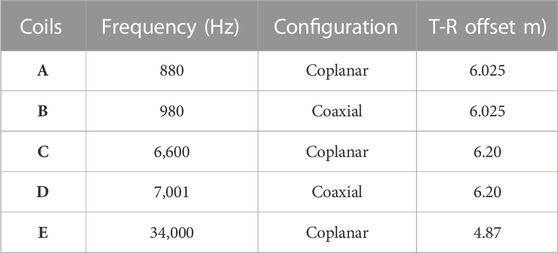
TABLE 1. Parameters of AEM system (Rønning et al., 2020).

2.2 Data preprocessing and network training

To obtain better training performance and accelerate the convergence, it is necessary to preprocess the training set before putting it into the neural network for training. Here we adopt the logarithmic normalization to keep the range of training data within [0, 1]. Specifically, for the resistivity parameters, we have

$Y_i=\frac{\log \left(Y_i\right)}{{\log \left(Y_i\right)}_{\mathit{max}}+a}(7)$

while for AEM data, we have

$X_i=\frac{\log \left(\left|X_i\right|\right)+b}{{\log \left(\left|X_i\right|\right)}_{\mathit{max}}+c}(8)$

where the parameters $a,b,c$ are introduced to ensure that the normalized parameters and data range from 0 to 1. These parameters should be chosen based on the ranges of the model parameters and the data in the training set. We then put the normalized training set into the training process shown in Figure 1. After that, we use an Adam optimizer (Diederik and Jimmy, 2014) to update the weights of the network and minimize the loss function to obtain the best training performance. In the network training process, we set the initial value of learning rate to ${10}^{-4}$ and the number of samples per batch to 32. The loss function used here is defined as the mean square error (MSE) of the difference between the model parameters and the predicted ones, i.e.

$\mathit{M}\mathit{S}\mathit{E}=\frac{1}{n}{\displaystyle \sum }_{i=1}^n{\left(Y_i-{\widehat{Y}}_i\right)}^2(9)$

where $Y_i$ and ${\widehat{Y}}_i$ represent respectively the true and the predicted resistivity model, $n$ denotes the number of samples in each batch.

FIGURE 1

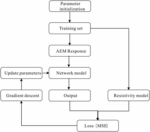
FIGURE 1. Flowchart of U-net training.

In the above network training process, we use the TensorFlow (Abadi et al., 2016) to establish the U-net network structure and perform the entire training process on a platform for data modeling and analysis at https://www.kaggle.com/. The GPU version accessed by this platform is Tesla P100-PCIE-16GB. Taking advantage of these supporting conditions, the training time required to loop a training set containing 100,000 samples for one epoch is approximately 60 s.

2.3 U-net architecture

The U-net has a “U" network structure. It was first used for the medical image segmentation. After that, it has also been successfully used in seismic data processing, inversion and interpretation in recent years (Yu and Ma, 2021). This method improves the traditional full convolution neural network (FCN) (Shelhamer et al., 2015). Its unique convolution operation can not only effectively reduce the large memory consumption caused by too many network layers, but can also largely reduce the number of weights and bias in the network, and thus ease the over fitting to the data.

The U-net architecture used for our training task is shown in Figure 2. Since the network input has a dimension of $32\times 10$ (including 32 measuring points and five frequencies with real and imaginary responses), we interpolate the input data into $32\times 16$, and then transpose it to match the output dimension of $16\times 32$. Considering that the sizes of our input and output data are small, too many down-sampling operations may lead to the loss of image information, which will reduce the positioning accuracy in the up-sampling process, we remove two down-samplings and up-samplings operations in the original U-net architecture. However, to solve the problem with insufficient extraction of high-level features due to fewer down sampling and convolutions, we added two convolution operations after each down-sampling.

FIGURE 2

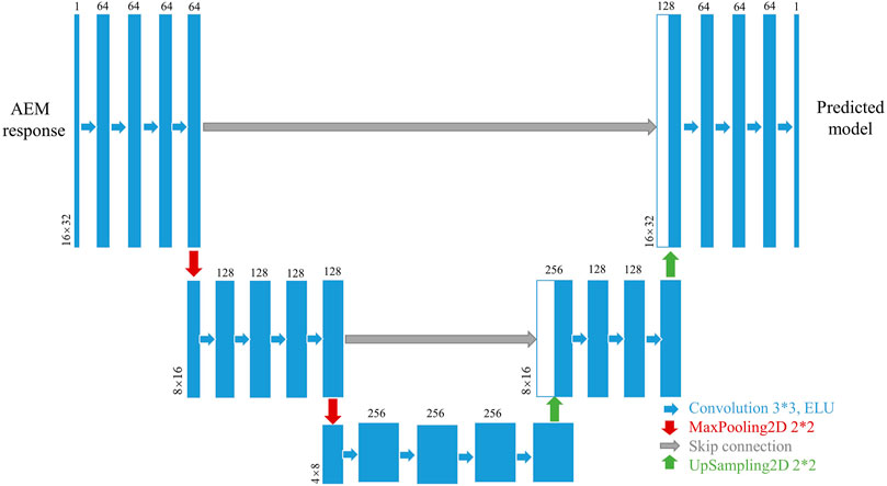
FIGURE 2. U-net network structure.

As shown in Figure 2, when we put AEM responses as input data into the trained U-net, the corresponding geoelectric model will be output after the forward propagation process. The numbers above and below each blue rectangle represent the number of channels and the data dimension of the current layer. The network used in our imaging process takes 64, 128, and 256 channels. The blue arrows represent the convolution operation shown in Figure 3. In each layer of convolution, we select the ELU (Exponential Linear Units) function (Clevert et al., 2015) as the activation function, so that the network has non-linear fitting capability. The red arrows represent the maximum pooling operations, as shown in Figure 4. The green arrows represent the up-sampling operations, which are the operations of data recovery via interpolations. The grey arrows represent the skip connections. This operation introduces the feature information on corresponding scales in the contracting path into the up-sampling process, so as to achieve feature fusion at different levels for a more precise imaging. It should be pointed out that in order to reduce the loss of edge information, we fill in all zeros to outside grids in each convolution operation to ensure that the data dimension will not be changed during the convolution process (see Figure 3).

FIGURE 3

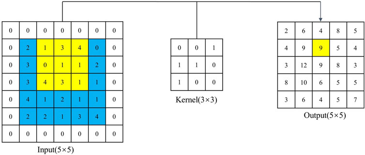
FIGURE 3. Zero padding and convolution process.

FIGURE 4

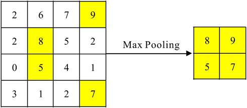
FIGURE 4. Maximum pooling process with a pooling size 2×2.

3 Theoretical data imaging

3.1 Model complexity analysis and verification of imaging results

In the following, we first validate our 2D imaging algorithm by synthetic data. As we know, the training set determines the performance of the network. The more complex the training set is, the more complex geological model the network can predict. Therefore, in this paper we establish two training sets with different complexities. The simple training set contains 50,000 samples, while the complex training set contains 100,000 samples. The model sizes of the two training sets are the same, both have $16\times 32$ grids, but the simple training set has uniform background and contains only one abnormal body. For the complex training set, we divide the background into upper and lower layers, with the layer interface being randomly set. In addition, we put up to three (0–3) abnormal bodies randomly in the layered background. As for the resistivities, we assign the background resistivity randomly within 1 Ω⋅m—10,000 Ω⋅m (logarithmically 0–9.21) and the abnormal resistivities within 1 Ω⋅m—1,000 Ω⋅m (logarithmically 0–6.91). Then, we randomly combine them into two cases: a conductive background with resistive anomalous bodies, and a resistive background with conductive anomalous bodies. After that, we take 1,000 samples from each training set to test the imaging effect of the network. The resistivity models used for testing do not participate in the network training.

After numerous tests, we find that 200 training epochs can deliver good imaging results. Figure 5 and Figure 6 respectively show the attenuation process of training errors and imaging results of the two training sets. From Figure 5 it is seen that the curves as a whole show a downward trend, the two curves of training set and validation set fit well with each other at the early training stage. However, as the training epochs increases, the loss error curves gradually get flattened. The minimum loss errors for the complex and simple training set reduce to .0015, .0017, respectively. From the imaging results shown in Figure 6, one sees that ether for a simple or more complex model, the neural network can very accurately establish the mapping relationship between the AEM responses and the underground resistivities, the layer interfaces and the boundaries of the abnormal bodies are clearly revealed, the predicted resistivities are also very close to the true values.

FIGURE 5

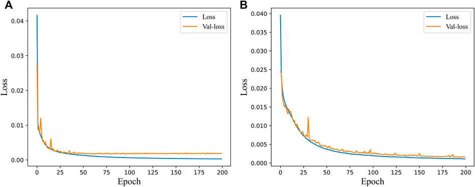
FIGURE 5. Loss errors versus epochs. (A) Simple training models (B) complex training models.

FIGURE 6

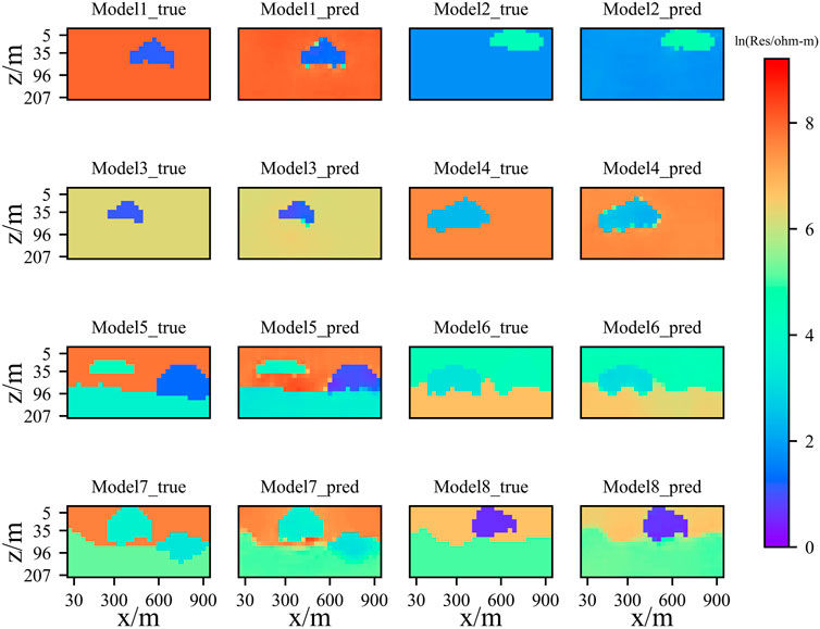
FIGURE 6. Imaging results for training sets of different complexities.

Model1∼Model4 are for a uniform background with a single body; Model5∼Model8 are for a complex background with multiple bodies.

To demonstrate the effectiveness of our imaging algorithm, we compare in Figure 7 the imaging results of theoretical data with the traditional inversions. From the comparison, we can see that the imaging results can clearly reveal the layer interfaces and anomalous boundaries, and deliver an image very close to the true model. The inversion results of Gauss-Newton (GN) method with a uniform half-space as the initial model can only roughly reveal the shape of the anomalous boundaries, the inverted resistivity is not accurate. Furthermore, the time consumptions for the GN inversion and our imaging method are quite different. While a single iteration in GN inversion takes several minutes on DELL workstation of Intel R) Xeon(R) Gold 6256 CPU at 3.60 GHz +3.59 GHz, while our imaging takes only seconds on the same equipment.

FIGURE 7

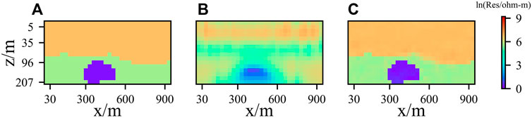
FIGURE 7. Comparison of imaging and inversion results. (A) True model (B) Gauss-Newton inversions (C) U-net imaging.

3.2 Effect of flight altitude on imaging results

In airborne EM, the flight altitude has a very significant impact on EM responses. To analyze the influence of flight altitude on the imaging of our network, we take 50,000 samples from the complex training set in Section 3.1 and calculate EM responses for four flight altitudes of 30, 50, 70, and 100 m for each model, so that the training set of 50,000 samples is expanded to 200,000. During the training process, we take the flight altitude as input in our network. After the network is trained for 200 epochs, the loss decreases to .0011 (see Figure 8).

FIGURE 8

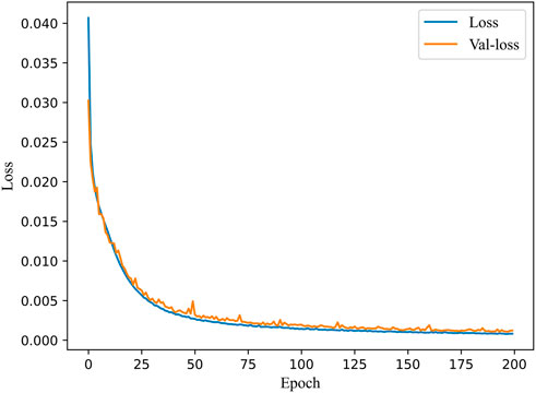
FIGURE 8. Loss versus epoch after flight altitude being added as input.

To check the effectiveness of our imaging method, we test the imaging results at three different altitudes of 40, 50, and 80 m. Among them, the flight altitude of 50 m has been seen by the network, while the altitudes of 40m and 80 m are not included in the training set and thus are unfamiliar to the network. Figure 9 shows the imaging results of AEM data for three flight altitudes. It is seen that no matter whether our network is familiar or unfamiliar with the flight altitude, it can obtain very accurate imaging results. However, when the network is familiar with the flight altitude the imaging results are better than those of the opposite cases. We can hope that with more AEM data for different flight altitudes being added to the training set, we will be able to improve the imaging results even for unfamiliar flight altitudes.

FIGURE 9

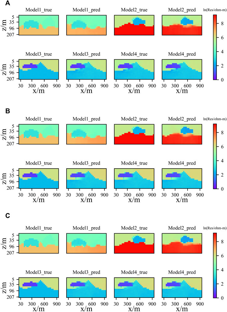
FIGURE 9. Imaging results for AEM data at different flight altitudes. (A)Imaging for unknown altitude of 40m (B) imaging for known altitude of 50m (C) imaging for unknown altitude of 80 m.

3.3 Effect of noise on imaging results

Until now, our imaging results are obtained from the theoretical data. However, AEM survey data are often contaminated by noise, so a stable and practical imaging method must have certain anti-noise capability. As we know, the neural network is sensitive to changes in the input data, and generally the longer the training time of a network is, the less adaptable to the interference of noise and the weaker the stability of the network is. Therefore, in this section we add different levels of Gaussian random noise (1%, 5%, 10%) to the test datasets used in the complex training set in Section 3.1. In addition to the aforementioned 200 epochs of model training, we train the training set for extra 50 epochs (the minimum error of the validation set is .0043). Then, we use the network to image the test set with different noise levels and analyze the influence of noise on the imaging results of the network. From the imaging results shown in Figure 10, we can see that when different levels of Gaussian noise are added to the test set, the network can characterize the boundaries of the anomalous body and the layer interfaces. This indicates that our U-net has certain anti-noise capability and can recover the model at different noise levels. However, analyzing the noise immunity of the network for different training epochs, we find that compared to the network with fewer training epochs, the network adaptability to noise with more training epochs is reduced. Although the network that underwent 200 training epochs achieves good imaging results when no noise was added, with increasing noise level, the depiction to the lower boundaries of the anomalous bodies begins to distort, and the layer interfaces begin to become blurred. In contrast, although the imaging results for 50 training epochs become slightly worse for noise-free data, they are less affected by the noise in the data.

FIGURE 10

FIGURE 10. Imaging results with different training epochs for data with different levels of noise. (A) True model (B–E) imaging results with 50 training epochs for the noise level of 0%, 1%, 5%, and 10% (F–I) imaging results with 200 training epochs for the noise level of 0%, 1%, 5%, and 10%, respectively.

Summarizing the above discussions, we can draw the conclusion that actually there exists a balance between the stability and accuracy of imaging results when using the network to image AEM data. As the noise level in the practical survey data cannot be accurately estimated, numerical experiments need to be done before starting processing AEM data, so that good imaging results can be obtained.

4 Field data imaging

To further verify the effectiveness of our network, we apply our imaging method to a survey dataset collected by the Norwegian Geological Survey in Byneset area, Norway (Rønning et al., 2020). Refer to Table 1 for the parameters of AEM system. Figure 11 shows the quaternary geological map of survey area. The blue part shows the marine sediments during the deglaciation period of about 10,000 years ago, which were exposed to the surface due to the rebound of glaciers. The 60 black lines represent AEM survey lines at a spacing of about 100 m. The distance between neighbor survey stations is 50 m. The line marked in red denotes the data segments used for our 2D AEM imaging.

FIGURE 11

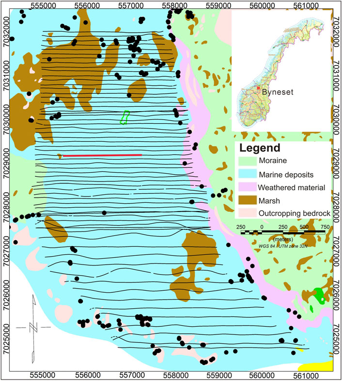
FIGURE 11. AEM survey area and survey lines in Byneset area, Norway (refer to Liu et al., 2018).

From the previous researches, we know that there exists a low-resistivity layer within the depth of 100 m in the survey area, which is the main geological feature in this area (Liu et al., 2018). To set up resistivity models that match the geology in the target area, we assume an undulating layered structure to replace the previous block model to construct the training set. Since the established training set only contains the layered structure with undulating layers, the mapping relationship becomes simpler than those of block anomalies, we only construct 10,000 samples for training, and accurate imaging results have been achieve on the test set. In addition, as the interval between neighbor survey stations is around 50m, we set the resistivity model in the training set with the lateral grid size and the spacing of survey points to 50 m. Totally, we have 32 survey points on each survey line. In Section 3.3, we have found that the noise in the data can have impacts on the imaging result, and the longer the training time is, the more serious this effect will become. After many experiments, we find that the network after 200 training epochs can obtain good imaging results. From the loss curves shown in Figure 12, one can see that the loss value is reduced to .0089 after 200 training epochs.

FIGURE 12

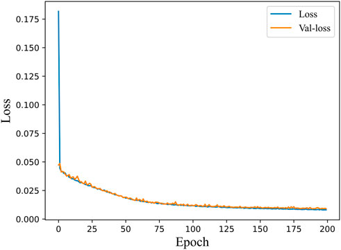
FIGURE 12. Loss versus epoch for the training set used to image the field survey data.

Before imaging the field survey data, we first test our trained network on synthetic data. Figure 13 shows the network imaging results for four different models. It is seen that the network well images the underground structures. The shapes and positions of the abnormal layers can be clearly identified. This implies that our network can work on more practical models with undulating layers.

FIGURE 13

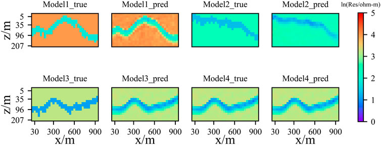
FIGURE 13. Imaging results for the synthetic data.

Figure 14 shows the comparison between the imaging results from this paper and those from the inversion based on the wavelet transform (Liu et al., 2018). It is seen that our imaging results based on U-net are consistent well with the inversion results from Liu et al. (2018). The resistivity obtained from the two methods are also very close. In addition, from the geological report for the survey area, we are informed that the top of the target area consists of a thin layer of marine sediments with the resistivity within 10 Ω⋅m - 50 Ω⋅m, underneath lies a thicker layer of conductive marine clay and under the marine clay lies the resistive bedrock. Our three-layer imaging results are well consistent with the geology in the survey area. This shows the effectiveness of our U-net network for imaging the AEM survey data. However, compared with traditional inversions that take large amount of time, our imaging method takes only a few seconds to process the data. This means that our imaging method can effectively improve the efficiency of AEM data interpretation, so that it will become possible to process AEM data in real time.

FIGURE 14

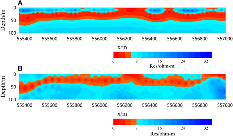
FIGURE 14. Imaging results of survey data acquired in Byneset area, Norway in comparison to the inversion results of Liu et al. (2018). (A) Inversion results (B) U-net imaging.

5 Conclusion

In this paper, we have successfully implemented a U-net neural network for 2D fast imaging of frequency-domain AEM data. The theoretical examples showed that the network can accurately establish the mapping relationship between AEM data and resistivity models and deliver accurate imaging results. In view of the particularity of AEM systems, we also examined the impact of the flight altitude on the imaging results and found that our network can provide better imaging results when the flight altitude is added to the training as a trainable variable. Moreover, the tests on noisy data also demonstrated that our U-net-based imaging algorithm has strong noise immunity. It can obtain reliable imaging results from noisy data even when no noise has been added to the training set. Finally, the experiments with the field survey data showed that the results obtained by our U-net imaging method are well consistent with 3D inversion results and the actual geology in the survey area, but at very low computational cost. This provides a solution to the practical low-efficiency problem in traditional AEM inversions.

Although the U-net presented in this paper can achieve fast and high-resolution 2D AEM imaging, however, the construction of the training set that matches the geology in the survey area is very important. This means that we need to have a prior geological information to set the model samples properly for the construction of training set, so that we can obtain good imaging results. If a more random model set-up strategy can be put forward in the future, or when the scale of the training set can be extensively expanded at large computational facilities, a training set with stronger adaptability to the complex underground structures can be established, the generalization ability of the network will be largely improved. At that time, we can expect that the real-time processing and interpretation of huge amount of AEM data become practical.

Data availability statement

The original contributions presented in the study are included in the article/supplementary material, further inquiries can be directed to the corresponding author.

Author contributions

QL implemented the algorithms, performed the analyses and wrote the manuscript. YL and CY came up with the idea of the method, supervised the study and review the manuscript. YS, LW, HL, and HW, helped in processing the data, discussing the results and drew the figures.

Funding

This paper was jointly funded by the National Natural Science Foundation of China (42030806) and the National Key R&D Program of China (2021YFB3202104).

Conflict of interest

The authors declare that the research was conducted in the absence of any commercial or financial relationships that could be construed as a potential conflict of interest.

Publisher’s note

All claims expressed in this article are solely those of the authors and do not necessarily represent those of their affiliated organizations, or those of the publisher, the editors and the reviewers. Any product that may be evaluated in this article, or claim that may be made by its manufacturer, is not guaranteed or endorsed by the publisher.

References

Abadi, M., Agarwal, A., Barham, P., Brevdo, E., Chen, Z., Citro, C., et al. (2016). TensorFlow: Large-scale machine learning on heterogeneous distributed systems. Available at: https://arxiv.org/abs/1603.04467 (Accessed March 16, 2016).

Google Scholar

Auken, E., and Christiansen, A. V. (2004). Layered and laterally constrained 2D inversion of resistivity data. Geophysics 69, 752–761. doi:10.1190/1.1759461

CrossRef Full Text | Google Scholar

Brodie, R., and Sambridge, M. (2004). Holistically calibrating, processing and inverting frequency domainAEM surveys[J]. ASEG Extended Abstracts, 2004, 1–4. doi:10.1071/ASEG2004ab014

CrossRef Full Text | Google Scholar

Cai, J., Qi, Y., and Yin, C. (2014). Weighted Laterally-constrained inversion of frequency-domain airborne EM data[J]. Chin. J. Geophys. 57, 953–960. doi:10.6038/cjg20140324

CrossRef Full Text | Google Scholar

Chen, J., and Raiche, A. (1998). Inverting AEM data using a damped eigenparameter method. Explor. Geophys. 29, 128–132. doi:10.1071/eg998128

CrossRef Full Text | Google Scholar

Clevert, D. A., Unterthiner, T., and Hochreiter, S. (2015). Fast and accurate deep network learning by exponential linear units (ELUs)[J]. Comput. Sci. doi:10.48550/arXiv.1511.07289

CrossRef Full Text | Google Scholar

Constable, S. C., Parker, R. L., and Constable, C. G. (1987). Occam’s inversion: A practical algorithm for generating smooth models from electromagnetic sounding data. Geophysics. 52, 289–300. doi:10.1190/1.1442303

CrossRef Full Text | Google Scholar

Diederik, K., and Jimmy, B. (2014). Adam: A method for stochastic optimization[J]. Comput. Sci. Available at: . https://arxiv.org/abs/1412.6980 (Accessed January 30, 2014).doi:10.48550/arXiv.1412.6980

CrossRef Full Text | Google Scholar

Farquharson, C. G., Oldenburg, D. W., and Routh, P. S. (2003). Simultaneous 1D inversion of loop–loop electromagnetic data for magnetic susceptibility and electrical conductivity. Geophysics 68, 1857–1869. doi:10.1190/1.1635038

CrossRef Full Text | Google Scholar

Gao, Z., Yin, C., Qi, Y., Zhang, B., Ren, X., and Lu, Y. (2018). Transdimensional Bayesian inversion of time-domain airborne EM data. Appl. Geophys. Bull. Chin. Geophys. Soc. 15, 318–331. doi:10.1007/s11770-018-0684-7

CrossRef Full Text | Google Scholar

Haber, E., Fohring, J., Mcmillan, M., and Granek, J. (2019). Using machine learning to interpret 3D airborne electromagnetic inversions[J]. ASEG Extended Abstracts, 2019. 1–4. doi:10.1080/22020586.2019.12072978

CrossRef Full Text | Google Scholar

Hodges, G., and Yin, C. (2007). Simulated annealing for airborne EM inversion. Geophysics 72, F189–F195. doi:10.3997/2214-4609.201401735

CrossRef Full Text | Google Scholar

Huang, H., Lin, L., Tong, R., Hu, H., Zhang, Q., Iwamoto, Y., et al. (2020). Unet 3+: A full-scale connected unet for medical image segmentation . ICASSP 2020-2020 ieee international conference on acoustics, speech and signal processing (icassp), 1055–1059. doi:10.1109/ICASSP40776.2020.9053405

CrossRef Full Text | Google Scholar

Huang, H., and Fraser, D. C. (1996). The differential parameter method for multifrequency airborne resistivity mapping. Geophysics. 61, 100–109. doi:10.1190/1.1574674

CrossRef Full Text | Google Scholar

Huang, H., and Rudd, J. (2008). Conductivity-depth imaging of helicopter-borne TEM data based on a pseudolayer half-space model. Geophysics. 73, F115–F120. doi:10.1190/1.2904984

CrossRef Full Text | Google Scholar

Iturrarán-Viveros, U., Muñoz-García, A. M., Castillo-Reyes, O., and Shukla, K. (2021). Machine learning as a seismic prior velocity model building method for full-waveform inversion: A case study from Colombia. Pure Appl. Geophys. 178, 423–448. doi:10.1007/s00024-021-02655-9

CrossRef Full Text | Google Scholar

Kobayashi, T., Oya, H., and Ono, T. (2002). A-scope analysis of subsurface radar sounding of lunar mare region. Earth, planets space EPS. 54, 973–982. doi:10.1186/bf03352445

CrossRef Full Text | Google Scholar

Li, J., Liu, Y., Yin, C., Ren, X., and Su, Y. (2020). Fast imaging of time-domain airborne EM data using deep learning technology. Geophysics 85, E163–E170. doi:10.1190/geo2019-0015.1

CrossRef Full Text | Google Scholar

Liu, B., Guo, Q., Li, S., Liu, B., Ren, Y., Pang, Y., et al. (2020). Deep learning inversion of electrical resistivity data. IEEE Trans. Geoscience Remote Sens. 58, 5715–5728. doi:10.1109/tgrs.2020.2969040

CrossRef Full Text | Google Scholar

Liu, Y., Farquharson, C., Yin, C., and Baranwal, V. (2018). Wavelet-based 3-D inversion for frequency-domain airborne EM data. Geophys. J. Int. 213, 1–15. doi:10.1093/gji/ggx545

CrossRef Full Text | Google Scholar

Macnae, J., King, A., Stolz, N., Osmakoff, A., and Blaha, A. (1998). Fast AEM data processing and inversion. Explor. Geophys. 29, 163–169. doi:10.1071/EG998163

CrossRef Full Text | Google Scholar

Macnae, J., and Lamontagne, Y. (1987). Imaging quasi layered conductive structures by simple processing of transient electromagnetic data. Geophysics 52, 545–554. doi:10.1190/1.1442323

CrossRef Full Text | Google Scholar

Meju, M. A. (1998). A simple method of transient electromagnetic data analysis. Geophysics 63, 405–410. doi:10.1190/1.1444340

CrossRef Full Text | Google Scholar

Minsley, B. J., Abraham, J. D., Smith, B. D., Cannia, J. C., Voss, C. I., Jorgenson, M. T., et al. (2012). Airborne electromagnetic imaging of discontinuous permafrost. Geophys. Res. Lett. 39 (0). doi:10.1029/2011gl050079

CrossRef Full Text | Google Scholar

Noh, K., Yoon, D., and Byun, J. (2020). Imaging subsurface resistivity structure from airborne electromagnetic induction data using deep neural network. Explor. Geophys. 51, 214–220. doi:10.1080/08123985.2019.1668240

CrossRef Full Text | Google Scholar

Puzyrev, V. (2018). Deep learning electromagnetic inversion with convolutional neural networks. Geophys. J. Int. 218, 817–832. doi:10.1093/gji/ggz204

CrossRef Full Text | Google Scholar

Ronneberger, O., Fischer, P., and Brox, T. (2015). U-Net: Convolutional networks for biomedical image segmentation. Med. Image Comput. Computer-Assisted Intervention – MICCAI 9351, 234–241. doi:10.1007/978-3-319-24574-4_28

CrossRef Full Text | Google Scholar

Rønning, J. S., Gautneb, H., Larsen, B. E., Baranwal, V. C., Davidsen, B., Engvik, A. K., et al. (2020). Geophysical and geological investigations of graphite occurrences in Vesterålen, Northern Norway in 2018 and 2019. NGU. NGU Report 2019.031. doi:10.13140/RG.2.2.31573.17126

CrossRef Full Text

Shelhamer, E., Long, J., and Darrell, T. (2015). Fully convolutional networks for semantic segmentation. Proceedings of the IEEE Conference Computer Vision Pattern Recognit. (CVPR), Boston, MA, June 07–12, 2015, 3431–3440. doi:10.1109/CVPR.2015.7298965

CrossRef Full Text | Google Scholar

Smith, R., O'connell, M., and Poulsen, L. (2004). Using airborne electromagnetics surveys to investigate the hydrogeology of an area near Nyborg, Denmark. Near Surf. Geophys. 2, 123–130. doi:10.3997/1873-0604.2004009

CrossRef Full Text | Google Scholar

Supper, R., Rmer, A., Jochum, B., Bieber, G., and Jaritz, W. (2008). A complex geo-scientific strategy for landslide hazard mitigation – from airborne mapping to ground monitoring. Adv. Geosciences 14, 195–200. doi:10.5194/adgeo-14-195-2008

CrossRef Full Text | Google Scholar

Tan, K., Munday, T., Halas, L., and Cahill, K. (2009). Utilising airborne electromagnetic data to map groundwater salinity and salt store at Chowilla, SA[J]. ASEG Extended Abstracts, 1–6. 2009. doi:10.1071/ASEG2009ab135

CrossRef Full Text | Google Scholar

ValléE, M. A., and Smith, R. S. (2009a). Application of Occam's inversion to airborne time-domain electromagnetics. Lead. Edge 28, 284–287. doi:10.1190/1.3104071

CrossRef Full Text | Google Scholar

Vallée, M. A., and Smith, R. S. (2009b). Inversion of airborne time-domain electromagnetic data to a 1D structure using lateral constraints. Near Surf. Geophys. 7, 63–71. doi:10.3997/1873-0604.2008035

CrossRef Full Text | Google Scholar

Van Der Baan, M., and Jutten, C. (2000). Neural networks in geophysical applications. Geophysics 65, 1032–1047. doi:10.1190/1.1444797

CrossRef Full Text | Google Scholar

Wang, J., Jun-Hua, Z., Jia-Liang, Z., Feng-Ming, L., Rui-Gang, M., and Zuoqian, W. (2021). Research on fault recognition method combining 3D Res-UNet and knowledge distillation. Appl. Geophys. 18, 199–212. doi:10.1007/s11770-021-0894-2

CrossRef Full Text | Google Scholar

Wolfgram, P., and Karlik, G. (1995). Conductivity-depth transform of GEOTEM data. Explor. Geophys. 26, 179–185. doi:10.1071/EG995179

CrossRef Full Text | Google Scholar

Yang, F., and Ma, J. (2019). Deep-learning inversion: A next-generation seismic velocity model building method. Geophysics 84, R583–R599. doi:10.1190/geo2018-0249.1

CrossRef Full Text | Google Scholar

Yin, C., Qi, Y., Liu, Y., and Cai, J. (2014). Trans-dimensional Bayesian inversion of frequency-domain airborne EM data[J]. Chin. J. Geophysics-Chinese Ed. 57, 2971–2980. doi:10.6038/cjg20140922

CrossRef Full Text | Google Scholar

Yin, C., Qiu, C., Liu, Y., and Cai, J. (2016). Weighted laterally-constrained inversion of time-domain airborne electromagnetic data[J], Earth Sci. Ed., 46., 254–261. doi:10.13278/j.cnki.jjuese.201601302

CrossRef Full Text | Google Scholar

Yin, C., Zhang, B., Liu, Y., Ren, X., Qi, Y., Pei, Y., et al. (2015). Review on airborne EM technology and developments[J]. Chin. J. Geophys. 58, 2637–2653. doi:10.6038/cjg20150804

CrossRef Full Text | Google Scholar

Yu, S., and Ma, J. (2021). Deep learning for Geophysics: Current and future trends. Rev. Geophys. 59, doi:e2021RG000742doi:10.1029/2021rg000742

CrossRef Full Text | Google Scholar

Zhu, W., and Beroza, G. C. (2019). PhaseNet: A deep-neural-network-based seismic arrival time picking method. Geophys. J. Int. 216, 261–273. doi:10.1093/gji/ggy423

CrossRef Full Text | Google Scholar